HAL Id: hal-00531205
https://hal-mines-paristech.archives-ouvertes.fr/hal-00531205
Submitted on 11 Mar 2011HAL is a multi-disciplinary open access
archive for the deposit and dissemination of sci-entific research documents, whether they are pub-lished or not. The documents may come from teaching and research institutions in France or
L’archive ouverte pluridisciplinaire HAL, est destinée au dépôt et à la diffusion de documents scientifiques de niveau recherche, publiés ou non, émanant des établissements d’enseignement et de recherche français ou étrangers, des laboratoires
A two-dimensional finite element thermomechanical
approach to a global stress-strain analysis of steel
continuous casting
Michel Bellet, Alban Heinrich
To cite this version:
Michel Bellet, Alban Heinrich. A two-dimensional finite element thermomechanical approach to a global stress-strain analysis of steel continuous casting. ISIJ international, Iron & Steel Institute of Japan, 2004, 44 (10), p. 1686-1695. �hal-00531205�
A two-dimensional finite element thermomechanical approach to
a global stress-strain analysis of steel continuous casting
Michel Bellet, Alban Heinrich
Ecole des Mines de Paris, Centre de Mise en Forme des Matériaux (CEMEF) UMR CNRS 7635
BP 207, 06904 Sophia Antipolis, France michel.bellet@ensmp.fr
Synopsis
This paper addresses the two-dimensional finite element simulation of steel continuous casting using a global non steady-state approach. The method aims at the calculation of the thermomechanical state (temperature, deformation, stresses) of steel all along the continuous casting machine. Both plane deformation and axisymmetric versions have been developed. The first one addresses the simulation of continuous casting of slabs, taking into account the possible curvature of the machine, whereas the second one applies to cylindrical billets. The implementation of the method is validated by comparison with results from the literature. It is applied to the study of a slab continuous caster for which successive depressive and compressive stress states are revealed in the secondary cooling region.
Key-words: continuous casting, finite elements, thermomechanics, stress-strain calculation ISIJ International 44 (2004) 1686-1695
Introduction
In the continuous casting (CC) of steel slabs or billets, liquid steel is poured into a bottomless mold. This water-cooled copper mold achieves the solidification of a shell, which is thick enough to permit downward extraction of the product. The material is then conveyed by supporting rolls throughout the so-called secondary cooling zone, in which it is cooled down by water spraying until complete solidification. In order to improve the process, in terms of both productivity and quality, steel producers have fostered the development of numerical models aiming at the prediction of the thermomechanical state (temperature, strains, stresses) of steel all along the primary and secondary cooling zone. There are two main reasons for that.
First, the knowledge of temperature, strains and stresses is required in order to evaluate the risk of initiation of surface cracks. As a matter of fact, the usual criteria or indicators for crack opening in solid state are based on local thermomechanical variables: temperature, stresses, strains, strain rates. Therefore, numerical models predicting those values for a given configuration (steel grade, caster geometry, extraction and cooling conditions) would help engineers to modify the process parameters (casting temperature and speed, intensity of water spray cooling, etc.), in order to reduce the risk of surface cracking. From the point of view of the manufacturers of CC machines, these models also could help in designing better machines, having an extended flexibility with respect to the format and the grades of the cast products. They would permit to test the influence of design parameters such as the curvature during bending and unbending, the dimensions of rolls, etc.
A second motivation lies in the fact that the bulging of the solidified shell of the product between supporting rolls has been shown to play a major role in the formation of centerline segregation 1). The numerical modeling of macrosegregation is beyond the scope of the present work, as it requires a two-phase liquid/solid thermomechanical approach including the coupling with the transport of chemical species. However, a prerequisite to any predictive analysis is a prediction of the bulging of the solidified shell, which is precisely the aim of the present work.
A global thermomechanical stress-strain analysis of the CC process is challenging, at least for two main reasons. On one hand, it is difficult to model steel behavior in a very large temperature interval, as researchers have not proposed yet reliable constitutive equations covering the different states encountered (liquid, mushy, solid). On the other hand, it is necessary to calculate on very large domains: because of the low thermal diffusivity of steel, the solidification depth ranges from 15 to 20 m for classical thick slabs (about 200 mm thick). The simulation then requires a huge computational power or parallel computation techniques. The paper presents a two-dimensional (2D) global thermomechanical finite element model. In a first part, we present a literature review about the different resolution strategies that have been developed so far, and we justify our choice of a global non steady-state method. Then the governing equations are presented and the proposed method is applied to different cases of industrial complexity, first to be validated by comparison with literature results and second to demonstrate the pertinence of the strategy and show its efficiency.
1 Resolution strategies for CC: literature review and present approach
Two main different strategies can be found in the literature: the non steady-state slice method, and the steady-state global approach.
1.1 Non steady-state slice method
In order to limit the number of unknowns, the slice method has been used by a great number of authors, among which Grill et al. 2), Kristiansson 3), Thomas et al. 4), Boehmer et al. 5). It consists in conveying throughout the machine a transverse section of the product: either a plane section or a volumic domain having a small thickness in the casting direction. Regarding heat transfer, top and bottom surfaces are adiabatic, the heat being extracted through the lateral boundary. As thermal gradients are very low along the casting direction in steel CC, this method yields good thermal results. However, it has major drawbacks regarding the mechanical analysis. Generally, a plane strain deformation state is assumed in the slice. Some authors, like Pascon 6) have extended this concept by assuming a state of generalized plane strain in order to cope with the bending and unbending. In spite of this, the slice approach does not take into account any shear effect and then cannot be representative of complex deformation states such as those associated with bulging. 1.2 Global steady-state method
An alternative consists of a Eulerian steady-state formulation, which operates on a quasi static computational domain covering the whole machine. This requires the integration of highly non linear constitutive equations (elastic-viscoplasticity) along streamlines, which needs specific advection methods, such as those proposed by Huespe et al. 7). In addition, such a problem is a free surface problem, since the location of the mesh boundary is unknown, because of bulging. Therefore specific algorithms must be used in order to move boundary nodes so that the velocity field be tangent to the surface. This has been done by Dalin and Chenot 8) but only on short isolated sections of the secondary cooling. In order to overcome this difficulty, Fachinotti and Huespe have proposed to keep the mesh identical in the analysis and to deduce the bulging a posteriori 7,9), which makes yet the steady-state formulation not fully consistent. In the authors’ opinion, it would be extremely challenging to develop a fully consistent free surface steady-state model, especially because of the contact conditions to be satisfied with a great number of rolls (typically more than 100). The convergence of such a problem might be extremely difficult. This is why it has been chosen to develop a new formulation, based on a non steady-state global formulation.
This new method, named GNS for short, is illustrated in Figure 1. Starting from an initial mesh representing a small amount of steel at the top of the machine, the advancing of the material is simulated by imposing to the lower surface a condition of bilateral contact with a rigid extraction tool. The upper surface remains fixed and then the mesh volume enlarges continuously with the casting speed. The extraction tool acts as the real bottom block which is used to initiate casting sequences. The proposed method is then close to that developed by Fjaer and Mo 10) or Li and Ruan 11) to study the starting phase of aluminum CC. However, in the present approach the prescribed boundary conditions should be chosen consistent with the steady-state regime. Therefore, adiabaticity and perfectly sliding bilateral contact conditions are imposed along the virtual extraction tool. This method thus requires solving a transient thermomechanical problem, which is supposed to converge towards the steady-state regime. It is thought that the GNS method, although computationally intensive, is well adapted to the above mentioned objectives, provided that a fast enough convergence to the steady-state regime can be observed, which will be discussed further. This approach has been implemented in the 2D finite element code R2SOL, developed at CEMEF in collaboration with Ecole des Mines de Nancy and SCC company. Details about this implementation can be found in reference 12).
Associated physical hypotheses and boundary conditions
At this stage, it is important to detail some assumptions that are closely associated with the GNS method. First, the model being focused on the thermomechanical stress-strain analysis, the fluid flow occurring in the liquid pool is ignored: we assume that whatever its state - liquid, mushy, or solid - the velocity of the material remains close to the nominal casting velocity. Of course this is a rough approximation in the liquid regions, especially in the mold, but we suppose that this assumption has no major impact on the thermomechanical state calculated within the secondary cooling, which is the effective aim of this work. From a mechanical and computational point of view, this is obtained by choosing a Newtonian model with a high enough viscosity in the liquid state. In addition, it is assumed that the liquid metal is equally distributed in the mold through the whole meniscus surface.
Mesh growth and boundary conditions
Let give now some details about the management of the mesh, which is a key-point of the method. As shown in Figure 1, the nodes belonging to the upper surface remain fixed, while all other nodes are of Lagrangian type: they move with the same speed as the material particles. Consequently the first row of elements near the top surface undergoes continuous elongation. To prevent mesh degeneracy, a remeshing operation is carried out, in which most nodes are untouched, except those located near the top surface. During remeshing, some new nodes are added in this region. The new fixed Eulerian nodes belonging to the top surface are then identified and the calculation goes on. From time to time, similar remeshings are achieved,
permitting a regular mesh growth. It should be noted that each remeshing is followed by a transport of the different thermomechanical variables from the old mesh to the new one. As most nodes are untouched, only the top region is affected by transport. It was found that this transport operation might generate significant errors when carried out just below the actual meniscus in the mold, because solidification often begins immediately below the meniscus. This is the reason why the top surface of the mesh is located slightly higher than the real meniscus, as shown in Figure 1: a “buffer” zone is then defined in which the steel is assumed to be perfectly homogeneous at the nominal casting temperature. Finally, the definition of associated mechanical boundary conditions should be discussed. As already said, the lower surface should satisfy a bilateral contact with the extraction tool. Regarding now the top surface, a definition of the boundary condition in terms of prescribed velocity field is not appropriate, because this velocity is simply unknown, as it results from the thermal contraction and solidification shrinkage of steel all along the caster, plus the bulging effects between rolls. Consequently, it is more appropriate to prescribe a pressure onto this surface. Neglecting the atmospheric pressure (i.e. the free surfaces are effectively free from any applied pressure) and denoting hb the height of the buffer zone, the
normal stress to be applied to the top surface is -ρlghb where ρl is the density at casting
temperature. Proceeding in this way, the pressure at the level of the actual meniscus is zero. 2 Heat transfer problem
The thermal problem is based on the resolution of the heat transfer equation, which is the general energy conservation equation, in which the source term associated with mechanical dissipation is neglected because of the very low strain rates encountered in the casting process:
) ( T dt dH ∇ ⋅ ∇ = λ ρ (1)
λ denotes the thermal conductivity, ρ the density and H the specific enthalpy which can be
defined as:
( )
d(
g)
L c H s T T p + − =∫
1 0 τ τ (2)with T0 an arbitrary reference temperature, cp the specific heat, gs the volume fraction of solid and
L the specific latent heat of fusion. In the present study, the solidification path gs(T) is considered
given. Therefore, the enthalpy can be calculated for any temperature value. 2.1 Thermal boundary conditions
Consider Ω the domain occupied by the growing mesh at a given instant t. The following conditions on its boundary ∂Ω are considered:
imp
T
T = (3)
This condition is applied onto the top surface of the mesh, where Timp is simply the
nominal casting temperature (see last paragraph of section 1.3). • Prescribed outward heat flux
imp
T φ
λ∇ ⋅ =
− n (4)
where n denotes the outward normal unit vector. • Convection ) ( ext c T T h T⋅ = − ∇ −λ n (5)
where Text denotes the external temperature and hc the convection coefficient. • Radiation ) ( 4 ext4 r r T T T⋅ = − ∇ −λ n ε σ (6)
where εr is the emissivity of the material (considered as a gray body), σr the
Stefan-Boltzmann constant. It is to be noticed that (6) can be cast in the same form as (5) by linearization, leading to a mixed convection-radiation boundary condition:
) ( ext cr T T h T⋅ = − ∇ −λ n (7) with ) )( ( 2 ext2 ext r r c cr h T T T T h = +ε σ + + (8)
Conditions (4) and (7) are applied to the lateral surface of the mesh, which is either facing the mold or submitted to the various conditions encountered in secondary cooling. In both cases, the values of heat flux or heat transfer coefficients are spatially averaged: between two metallurgical lengths (i.e. curvilinear abscissa along the caster), those values are assumed constant and supposed to be representative in average of the different heat transfer phenomena. In other words, a detailed analysis of thermal boundary conditions (contact with rolls, spray aspersion, calefaction) has not been considered here. However, following Hardin et al. for instance 13), such complements could be implemented in the present model, in order to increase its accuracy. Finally, as already mentioned in section 1.3, an adiabatic condition is applied to the bottom surface in contact with the virtual extracting tool. It should be noted here that the aim of the present analysis is not to be representative of the actual heat transfer occurring between the material and the starting block during the transient effective initiation of the casting. This is another interesting problem, but which would need to calculate heat conduction in the starting block as well. The selected adiabatic condition is more appropriate to the GNS approach especially when a fast convergence to the steady-state regime is aimed at.
2.2 Resolution
The standard Galerkin discretization leads to the classical set of non linear equations: Q
KT H
M& + = (9)
with M the mass matrix, K the conduction matrix, Q the right hand side vector, H& the vector of enthalpy rates at nodes and T the vector of nodal temperatures. The phase change affecting the material is treated using the technique proposed by Lemmon 14). Applying this technique to linear elements (P1 triangles), an element-wise constant value of the effective heat capacity is approximated by the following regularization formula:
T T H T H ceff ∇ ∇ ≈ ∂ ∂ = ( ) (10)
The set of equations (9) then becomes:
Q KT T
C&+ = (11)
with T& the vector of nodal temperature rates, C the heat capacity matrix. This latter matrix is then temperature dependent within the solidification interval (and possibly outside, due to cp
variations). In addition, matrix K and vector Q may depend on temperature. A Euler backward implicit time discretization scheme leads to a set of non linear equations which is solved by a Newton-Raphson method for the nodal temperatures at the end of the time increment considered:
0 ) ( t+∆t = heat T R (12) 3 Constitutive equations
Most earlier works dealing with stress-strain numerical modeling in steel-CC were based on elastic-plastic or elastic-viscoplastic constitutive equations. This approach is valid provided that the calculations are limited to the regions where steel is solidified. In this case, elastic-viscoplastic models give a better response than elastic-plastic models because they include strain rate sensitivity at high temperature. However it should be pointed out that this approach is no more valid when it is extended to regions where steel is in the mushy (semi-solid) or in the liquid state. In this case, the material essentially behaves like a fluid. This is the reason why we will consider here, like in other simulations of solidification processes 15) a hybrid constitutive model. 3.1 Hybrid liquid-solid constitutive model
Liquid and mushy state
Above solidus temperature, a pure thermo-viscoplastic model is used: it is described by the following equations.
th vp
ε ε
s εvp eq m K − = 1 2 3 ε& & (14) I ε ∆ + = tr s th g T ε α& & & 3 1 (15) No elasticity is accounted for. As the strain rate tensor ε& is split into a viscoplastic and a thermal part (13), the change in the density of the material is only due to this thermal contribution which comprises the effect of thermal expansion (T& denotes the temperature rate, α the thermal linear expansion coefficient, I the identity tensor) and solidification shrinkage (g& denotes the rate of s the volumic solid fraction, ∆εtr
the relative volume change due to the total liquid-solid transition). Equation (14) is the classical constitutive equation of a generalized non Newtonian fluid. It relates the viscoplastic strain rate to the stress deviator s, which is in turn defined by:
σ I σ s tr 3 1 − = + = p p (16)
in which σ is the Cauchy stress tensor and p the associated hydrostatic pressure. In (14), K is the so-called consistency of the material and m is the strain rate sensitivity coefficient, while ε& is eq the von Mises equivalent strain rate, defined by:
vp ij vp ij eq ε ε
ε& & & 3 2
= (17)
From (14), the following power-law type one-dimensional form can be obtained:
m eq
eq Kε
σ = & (18)
in which σeq is the von Mises equivalent stress defined by:
ij ij eq s s 2 3 = σ (19)
The limit case of the Newtonian behavior (liquid state) is obtained for m = 1. In this case, K is equal to the dynamic viscosity of the liquid multiplied by a factor 3.
Solid state
Below solidus temperature, a thermo-elastic-viscoplastic model is used to represent the behavior in the solid state. It is described by the following equations:
th vp el ε ε ε
ε&=& +& +& (20)
I σ σ
ε& 1 & tr(&) E E el = +ν −ν (21) s ε m n eq eq eq vp K 1 0 2 3 ε σ σ σ − = & (22)
I
ε&th =αT& (23)
The strain rate tensor ε& is split in an elastic, a viscoplastic, and a thermal part (20). As in the fluid-like model, the latter includes thermal expansion (23). Equation (21) yields the hypoelastic Hooke's law, where E is the Young's modulus, ν the Poisson's coefficient and σ& a time derivative of the stress tensor. Equation (22) gives the relation between the viscoplastic strain rate and the stress deviator s. From (22), the following one-dimensional form can be obtained:
m eq n eq eq σ Kε ε σ = 0 + & (24) 0
σ denotes the static yield stress below which no viscoplastic deformation occurs (the expression between brackets in (22) is reduced to zero when negative). The contributions of strain hardening and strain rate are combined in a multiplicative way. It should be noted that an alternative expression of (22) is available in the numerical model, resulting in additive contributions of strain hardening and strain rate 12,15).
4 Mechanical equilibrium equations
At any time, the local mechanical equilibrium is governed by the equation of momentum conservation, in which inertia effects are neglected according to the above mentioned hypothesis regarding the modeling of the liquid state. Denoting g denotes the gravity vector, we have:
0 = + ∇ − ⋅ ∇ = + ⋅ ∇ σ ρg s p ρg (25)
4.1 Mechanical boundary conditions
At any time t, the following conditions on the boundary ∂Ω of the domain are considered: • Prescribed pressure
n σn
T = =−pimp (26)
This condition is applied onto the top surface, with pimp =−ρlghb, as already mentioned. • Sliding bilateral contact
This condition is applied to the bottom surface, which is in contact with a virtual extraction tool moving at the nominal casting speed vcast. In a first approach this condition amounts to the prescription of the normal component of the velocity vector:
cast
v = ⋅n
v (27)
Actually, if the machine is curved, the condition is applied in a slightly different manner because of the incremental treatment 12). The contact is assumed to be perfectly sliding in the tangential direction.
This condition is applied to the lateral surface in order to model contact with either the mold or the rolls, which are all considered as non deformable obstacles. The equations for unilateral contact are as follows:
= ⋅ ≥ ≤ ⋅ 0 ) ( 0 0 δ δ n σn n σn (28)
where δ is the signed distance to the obstacle (negative in case of penetration) and n is the local outward unit normal to the cast product. The fulfillment of (28) is obtained by means of a penalty condition, which consists in applying locally a repulsive normal stress vector to the surface of the product each time the proposed velocity field leads to a penetration of the obstacle. In case of contact with the mold, the normal stress vector is proportional to the local penetration via a penalty constant χp (like in (22) the brackets
denote the positive part):
n σn
T = =−χp −δ (29)
In case of contact with a roll, it is expressed as follows, according to Figure 2. CM R p − = − = = = r r r r σn T χ δ with δ and (30)
where C denotes the center of the roll section, R its radius and M is the position of the considered material point. Therefore the unilateral condition is expressed using the analytical circular shape of the roll. In addition, in order to stabilize the contact treatment, the multiplier χp is assigned to each roll. The value of χp is modified incrementally in
order to monitor the numerical penetration (-δ) of the cast product into the roll around a prescribed value denoted penobj, which is typically chosen equal to 0.1 mm. Assuming
that the contact pressure against the roll evolves slowly, the change of χp between to
successive time increments ν and ν +1 is defined by:
obj p p pen ) ( 1 ν ν ν χ δ χ + = − (31)
If the current penetration (−δν) is close to penobj, the correction of χp is small;
conversely, the ratio χνp+1/χνp is arbitrary limited to the interval [0.1 ; 10] in order to
avoid abrupt changes. In CC, this strategy has been found better than the usual penalty or augmented Lagrangian methods in which either χp is a constant or each surface node has a
variable χp. The reason is that the contact of a surface node with successive rolls is
intermittent. At each roll there is not enough time or increments to adjust correctly the value of χp attached to the streaming node: the penetration cannot be controlled.
Inversely, the assignment of χp to the rolls yields a controlled regular numerical
In the present work, no tangential friction has been considered. The motorization of certain rolls of the caster is also ignored. Those interesting features have been implemented in some numerical models 6) and should be integrated in the proposed model in the future.
4.2 Weak form of mechanical equations
The primitive variables are velocity and pressure. The problem to be solved is then composed of two equations. The first one is the weak form of the momentum equation (25). Since p is kept as a primitive variable, only the deviatoric part of constitutive equations is accounted for and has to be solved locally in order to determine the deviatoric stress tensor s. The second equation consists of a weak form of the volumetric part of the constitutive equations. It expresses the incompressibility of the plastic deformation. This leads to:
= ∀ = ⋅ − ⋅ − ⋅ ∇ − ∀
∫
∫
∫
∫
∫
Ω Ω Ω ∂ Ω Ω 0 tr 0 : * * * * * * * dV p p dV dS dV p dV vp ε v g v T v ε s v & & ρ (32)in which s: ε& denotes the contracted product of the two second order tensors: * * ij ijε
s & . The pressure appears as a Lagrange multiplier of the incompressibility constraint. The term integrated in the second equation changes according to the local state of steel (i.e. according to temperature): the stress deviator s results either from an elastic-viscoplastic constitutive relation ((20)-(23)), or from a viscoplastic or Newtonian law ((13)-(15)). After space discretization with the triangular mini-element (P1+/P1) 12,15,16), (32) can be cast in a set of non linear equations the unknowns of which are V, vector of nodal velocities and P, vector of nodal pressures:
0 ) , (V P =
Rmech (33)
This set of non linear equations is solved by a Newton-Raphson method. The motion of the mesh is then governed by a time integration of the velocity over the time step. The new location of each node n, except those located at the top surface, which remain fixed, is defined by:
n t n t t n X tV X +∆ = +∆ (34) 5 Results
5.1 Heat transfer analysis
In a first approach, we focus on the heat transfer analysis, in order to validate the GNS method. This is obtained by comparison with a slice method, both being operated with the same code R2SOL. The comparison is carried out for a slab caster (thickness 222 mm ; 0.06%C-0.4%Mn
steel ; liquidus 1528 °C ; solidus 1495 °C ; casting velocity 20.8 mm/s ; initial temperature 1547 °C), using a simplified material data set (linear solidification path, heat conductivity 30 W.m-1.K
-1
, density 7300 kg.m-3, specific heat 675 J.kg-1.K-1, latent heat 260000 J.kg-1). The considered slice has a thickness of 10 mm in the casting direction. It consists of a structured mesh of triangles (mesh size around 5 mm, 45 nodes in the slab thickness direction and 3 in the casting direction ; total number of elements 176). The GNS method is carried out with an initial mesh of uniform mesh size 10 mm. The buffer zone is 200 mm high. In both methods, plane strain conditions are assumed. They are representative of the conditions found in the median longitudinal plane of the slab. In each point, the velocity vector belongs to this plane, and the velocity components don’t depend on the third spatial coordinate, in the normal direction to the plane. Both mechanical and thermal resolutions are performed at each time increment but it should be noticed that the only role of the mechanical resolution in this case is to convey the material through the caster. Therefore, the choice of the constitutive model is of minor importance. For the sake of simplicity a pure Newtonian constitutive behavior with an arbitrary high viscosity has been chosen. In the case of the slice method, the gravity has been ommitted in order to avoid the fall of the thin slice between the rolls: the slice is then simply guided by the extraction tool.
Figure 3 illustrates the growth of the computational domain when using the GNS method. The computation has been carried out up to 24 min, corresponding to a metallurgical length of 30 m. The time step has been kept constant equal to 1 s and the total computation time is 15 hours on a 2.5 GHz Pentium4 PC. By the end of the computation the mesh has around 50000 nodes.
In order to study the convergence to the steady-state regime, the temperature evolution is examined in three different locations at a metallurgical length of 7 m: in the center of the slab, on the surface (on the outer side) and at mid-distance. In Figure 4, it can be seen that the steady-state regime is obtained quasi immediately after the virtual extraction tool (i.e. the lower end of the product) has reached this metallurgical length. Then, because of successive interpolations performed onto a streaming mesh, the temperature fluctuates around a constant average value. We can see that only the center temperature is free from fluctuations, the temperature gradient being extremely low at this point. This rapid convergence is a key-result regarding the application of the GNS method: it means that it is not necessary to let the calculation go on far beyond a given length to get a pertinent steady-state temperature profile at this length. In Figure 5 the two methods are compared. The calculated temperature evolution at the center of the slab and the outer skin is studied. It can be seen that the results obtained by the two methods are very close. The difference may come from the mesh size, which has been taken smaller in the slice-type analysis. This validates the implementation of the GNS method.
5.2 Thermomechanical analysis: stress-strain analysis during primary cooling in the mold In this section, we focus on the thermomechanical analysis in the primary cooling in the case of axisymmetric billets of 0.28%C-1.3%Mn steel. The geometry is given in Figure 6 and the
thermophysical parameters and boundary conditions are those used by Fachinotti and Huespe 7,9). This case is used as a validation test for the implementation of the mechanical resolution in R2SOL software, using the GNS method. The casting velocity is 26.67 mm.s-1 and the casting temperature is 1530 °C. The simulation conducted by Fachinotti is of Eulerian steady-state type, the fixed mesh being limited to a distance of 1 m under the meniscus. Only the solid region is considered: the mesh is restricted to the region where the temperature is lower than the so-called “zero-strength temperature” (ZST, 1495 °C), 5 °C above solidus (1490 °C). This region is deduced from a preliminary pure heat transfer analysis, and then meshed with linear triangles in a structured manner.
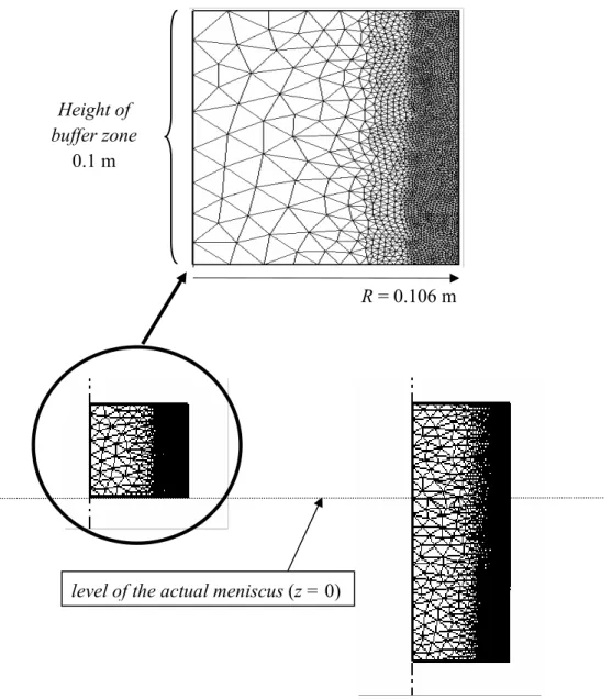
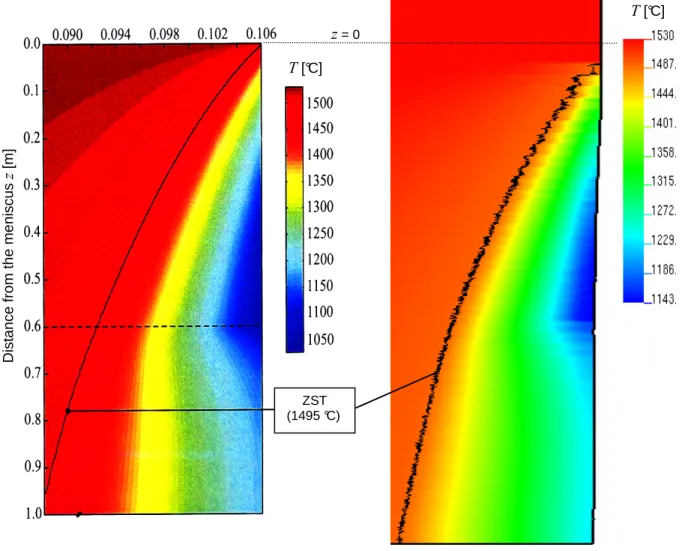
The R2SOL computation is carried out using the GNS method. Because of axisymmetry, the computational domain is restricted to positive radial coordinates. Figure 7 shows the evolution of the mesh, which is refined near the mold interface (1.5 mm, against 20 mm in center). The mesh size used is coarser than the one used by Fachinotti. The buffer zone is 0.1 m high and the calculation has been done until a metallurgical length of 1.1 m down under the meniscus, the mesh including then about 40000 nodes, for a computation time of 4 hours (constant time step 1 s). The comparison of the temperature distribution calculated by the two models in a 18 mm band near the mold interface is shown in Figure 8. A good agreement is found between the two approaches, in view of the differences in the mesh size. Regarding the thermomechanical results, Figure 9 gives a comparison of the distributions of axial stresses calculated in the same region by both methods. The same global agreement is found, except at the bottom of the mold. The reason is the following: using the Eulerian method, the stresses are calculated on a fixed mesh, whereas with the GNS method, the unilateral contact is treated, causing an air gap visible on the figure. Although this gap has no influence in this case on the temperature profile, because the boundary condition at the interface consists of a prescribed heat flux, there is a clear influence on the stress distribution. Similar conclusions can be drawn from the comparison of hoop stresses. These results validate the implementation of the mechanical resolution for the GNS method, which can now be applied to a curved slab caster.
5.3 Thermomechanical analysis: stress-strain analysis during secondary cooling
A coupled thermomechanical analysis has been performed on the same casting geometry and material as in section 5.1. The considered low carbon steel solidifies in δ-Fe (liquidus 1528 °C, solidus 1495 °C). According to the Thermocalc software 17), the δ/γ transformation begins after the solidification is completed, between 1473 °C and 1439 °C. In the solid state, the parameters K, n and m of the viscoplastic constitutive equations of δ-Fe over 1473 °C and of γ-Fe below 1439 °C have been directly derived from the work of Kim et al. 18), in which the static yield stress σ0 is assumed to be zero. In the temperature interval of the δ/γ transformation, a mixing law is
applied, taking into account the volume fraction of each phase 12). Regarding the elasticity parameters, the temperature dependence of the Young modulus E has been taken from the work of Kozlowski et al. 19), while a constant arbitrary value of 0.3 has been chosen for the Poisson
coefficient ν. The thermal expansion coefficient α and the shrinkage ratio ∆εtr have been deduced from the temperature dependence of the density ρ, which has been supplied by ARCELOR, one of the industrial partners of this study. In the semi-solid state, constant values of K and m have been arbitrarily assumed between solidus and the temperature at which the solid fraction is 0.7 (1519 °C). Above this temperature a linear variation of ln K and of m has been arbitrarily assumed up to liquidus, for which K = 500 Pa.s and m = 1. The appendix contains the detailed values of all rheological parameters. Regarding contact with rolls, the authorized numerical penetration has been fixed to 0.1 mm. The mesh size is non homogeneous (8 mm near the surface, 20 mm in the center). Like in section 5.1, plane strain conditions are assumed.
Compression and depression in the solid shell
In Figure 10, the middle of the secondary cooling zone is examined, at a metallurgical length of about 11 m. The alternation of compressive and depressive zones is evident by looking at the pressure distribution. Actually, the results obtained show a double alternation. First, in surface, the material is in a compressive state under rolls where the pressure reaches its maximum, 36 MPa. Conversely, it is in a depressive (tensile) state between rolls, where the pressure is minimum (-9 MPa). If we look now at the pressure state still in the solid shell but close to the solidification front (i.e. close to the solidus isotherm), we can see that there is also an alternation, but opposite: the steel is in a tensile state (negative pressure of about –2 MPa) when passing in front of rolls, while it is in a compressive state in between, the value of pressure being around 2 to 3 MPa. These results are in agreement with previous structural analyses of the deformation of the solidified shell between rolls, such as those carried out in static conditions by Wünnenberg 20), Dalin and Chenot (in three dimensions) 8), Miyazawa and Schwerdtfeger 1), or by Kajitani et al.
21)
on limited slab sections moving downstream between rolls and submitted to the metallurgical pressure onto the solidification front.
Deflections between rolls
The calculated deflections on both sides of the product are shown in Figure 11, when the extracted length has reached 20 m. The vertical lines indicate the location of rolls and it can be seen that the contact is well managed, the calculated deflections at roll locations being maintained all along the caster close to the value of the objective penetration penobj (0.1 mm). This shows the
efficiency of the proposed formulation, especially the automatic updating of the penalty coefficient assigned to each roll. The amplitude of the net deflection is around 0.2 mm. In reference 12), it has been checked that the calculated net deflection remains identical when slightly increasing the radius of each roll by a value of 0.1 mm. Doing so, the deflection at each roll with respect to the real roll surface location is very close to zero. This also shows that the net bulging is sufficiently independent on the choice of the numerical penetration penobj. Unfortunately, no
experimental bulging measurement is available at that time, but the order of magnitude is in agreement with the estimations of the engineers in charge of the caster in production.
Like the stabilization of the temperature field, the stabilization of these deflections has been investigated. Figure 12 gives a typical evolution of the deflection. Contrary to the temperature field, there exists a time interval before the convergence around an average value is obtained. It has been found that this duration varies with the casting speed, whereas the length associated with the stabilization (that is the stabilization duration multiplied by casting velocity) remains constant, which sounds logical. This length is about 2 m, that is approximately 10 % of the total length, which is acceptable. The causes of this progressive stabilization are the followings. First, the mechanical condition applied to the product end clearly has an influence. Second, the non penetration condition into the rolls is progressively obtained, by incremental modifications of the penalty coefficient associated with each roll. In order to facilitate the convergence of the mechanical resolution, this coefficient is initialized to a rather low value, which causes an initial rather high penetration in the roll (as it can be seen on Figure 12). Then a certain time is needed to control penetration. Third, contrary to heat transfer, gradients of mechanical variables do exist in the casting direction. Therefore a given length is needed in order to get free from the end effect associated with contact with the extraction tool. A zoom on the shape of the free surface in two successive roll intervals is given in Figure 13, showing a non-smooth surface profile. Current work is in progress to analyze the origin of such oscillations, which are probably related to space and time discretization. However, the averaged profile, as drawn on the figure, is shifted in the downstream direction, which is in agreement with the literature 1,8,20,21).
Final discussion and conclusion
An original approach to the thermomechanical stress-strain analysis of steel CC has been developed. Based on a GNS method, it has been implemented in a 2D finite element software in order to calculate the deformations and stresses affecting the cast products, either in plane strain or axisymmetric conditions. The treatment of contact with mold and rolls permits to account for the actual geometry of industrial casters. In particular, the contact with rolls has been treated by an original penalty method in which a penalty coefficient is assigned to each roll and modified incrementally. The efficiency of this method has been demonstrated on an industrial case, for which the numerical penetrations in rolls are very well uniformly controlled all along the secondary cooling. Although it is based on a non steady-state approach, the calculation converges rapidly to the steady-state regime, which is a key-point to achieve simulations at a reasonable computation cost. After a validation step, the proposed approach has been applied to the stress-strain calculation in the case of a thick slab vertical-curved machine. The main result is the evidence of successions of depressive and compressive states encountered by the material when passing between the rolls. This phenomenon affects the solid shell throughout its thickness, showing that it effectively behaves like a beam loaded by the internal metallurgical pressure and resting on the rolls. Although this phenomenon had already been described in the literature, it is
the first time, up to our knowledge, that it is calculated in a global thermomechanical simulation of the secondary cooling.
The advantages and drawbacks of the proposed GNS formulation, compared to alternative methods, can be summarized as follows:
− The GNS method gives access to the steady-state thermomechanical state of the solidified shell in the entirety of the caster: temperature, liquid fraction, components of stress and strain rate tensors, von Mises stress and strain rate.
− It takes into account the actual geometry of the caster: mold, curvature, supporting rolls. − Despite its non steady-state nature, it converges quickly towards the steady-state regime. It
could also be used to model the transient regime of the beginning of a casting sequence. − The GNS method is superior to the non steady-state slice-type method, in which the boundary
conditions are ill-posed, shear is not accounted for and bulging prediction is impossible. − Steady-state thermomechanical analyses may offer a good alternative. However, they have
never been applied to the entirety of a machine. They have been used to focus on the mold region for the study of the primary shell, or on a few roll intervals to study bulging. In the latter case, they suffer from a crucial problem, which is how to initialize the stress state, as the thermomechanical history of the material remains unknown.
Finally, beyond the present results, complementary developments are needed in order to overcome the current limitations of the proposed GNS model:
− Some mechanical boundary conditions of the present model should be improved: friction in the mold, friction with rolls, motorization of certain rolls.
− Similarly, the thermal boundary conditions could be modeled more accurately, by using different heat exchange coefficients associated with the different conditions encountered by the material: roll contact, water spray, calefaction, convection and radiation.
− Up to now the sensitivity to the mesh size has not been fully evaluated and this should be studied in more detail in the future.
− The current thermomechanical model used in the mushy state is very rough, since it is based on a one-phase approach, the alloy obeying a pure viscoplastic constitutive equation within the solidification interval. Some work is in progress in order to improve it by modeling the mushy alloy as a two-phase continuum, with an effective distinction between the motion of the liquid phase and of the solid phase 22).
− Although still computationally expensive, the 3D GNS approach is being developed 23). − The modeling of the mold region could be improved, including the coupling between fluid
flow and solidification of the primary solid shell, which remains a challenging problem. Acknowledgement
The authors would like to acknowledge the financial support of companies ARCELOR and ASCOMETAL and of the French Ministère de l’Economie, des Finances et de l’Industrie, in the frame of the OSC-CC project.
References
[1] K. Miyazawa and K. Schwerdtfeger: Arch. Eisenhüttenwes., 52 (1981) 415-422.
[2] A. Grill, J.K. Brimacombe and F. Weinberg: Ironmaking and Steelmaking, 1 (1976) 38-47. [3] J.O. Kristiansson: J. Thermal Stresses, 7 (1984) 209-226.
[4] B.G. Thomas, W.R. Storkman and A. Moitra: Proc. 6th Int. Iron and Steel Congress, Nagoya, Iron and Steel Institute of Japan (1990) 348-355.
[5] J.R. Boehmer, G. Funk, M. Jordan and F.N. Fett: Advances in Engineering Software, 29 (1998) 679-697.
[6] F. Pascon: 2D1/2 thermal-mechanical model of CC of steel using the finite element method. Ph.D. Thesis, University of Liège, Belgium (2003).
[7] A.E. Huespe, A. Cardona and V.D. Fachinotti: Comput. Meth. Appl. Mech. Engng., 182 (2000) 439-455.
[8] J.B. Dalin and J.L. Chenot: Int. J. Num. Meth. Engng., 25 (1988) 147.
[9] V.D. Fachinotti: Modelado Numerico de fenomenos termomecanicos en la solidificacion y enfriamento de aceros obtenidos por colada continua, Ph.D. thesis (in Spanish), Universidad Nacional del Litoral, Santa Fe, Argentina (2001).
[10] H.G. Fjaer and A. Mo: Metallurgical Transactions B, 21 (1990) 1049-1061. [11] B.Q. Li and Y. Ruan: J. Thermal Stresses, 18 (1995) 359-381.
[12] A. Heinrich: Modélisation thermomécanique de la coulée continue d’acier en deux dimensions, Ph.D. Thesis (in French), Ecole des Mines de Paris (2003).
[13] R.A. Hardin, H. Shen and C. Beckermann: Proc. 10th Int. Conf. on Modeling of Casting, Welding and Advanced Solidification Processes, The Minerals, Metals & Materials Society, Warrendale, Pennsylvania (2003) 729-736.
[14] E.C. Lemmon: Numerical Methods in Heat Transfer, J. Wiley and Sons (1981) 201-214. [15] M. Bellet, O. Jaouen: Proc. Int. Conf. on Cutting Edge of Computer Simulation of
Solidification and Casting, Osaka, The Iron and Steel Institute of Japan (1999) 173-190. [16] O. Jaouen: Modélisation tridimensionnelle par éléments finis pour l’analyse
thermomécanique du refroidissement des pièces coulées, Ph.D. Thesis (in French), Ecole des Mines de Paris (1998).
[17] B. Sundman: Thermocalc user’s guide, Division of Computational Thermodynamics, Department of Materials Science and Engineering, Royal Institute of Technology, Stockholm (1997).
[18] K.H. Kim, K.H. Oh and D.N. Lee: Scripta Materialia, 34 (1996) 301-307.
[19] P.F. Kozlowski, B.G. Thomas, J.A. Azzi and H. Wang: Metallurgical Transactions A, 23 (1992) 903-918.
[20] K. Wünnenberg: Stahl und Eisen, 6 (1978) 254-259.
[21] T. Kajitani, J.M. Drezet and M. Rappaz: Metallurgical and Materials Transactions A, 32 (2001) 1479-1491.
[22] S. Le Corre, M. Bellet, F. Bay and Y. Chastel: Proc. 10th Int. Conf. on Modeling of Casting, Welding and Advanced Solidification Processes, The Minerals, Metals & Materials Society, Warrendale, Pennsylvania (2003) 345-352.
[23] F. Costes, A. Heinrich and M. Bellet: Proc. 10th Int. Conf. on Modeling of Casting, Welding and Advanced Solidification Processes, The Minerals, Metals & Materials Society, Warrendale, Pennsylvania (2003) 393-400.
Appendix: rheological data used for the 0.06%C-0.4%Mn steel Solid state
K, m and n (from Kim et al. 18))
T [°C] K [MPa.s-m] T [°C] m [-] n [-] 845 859.4 845 0.201 0.429 895 635.4 1439 0.201 0.429 945 481.6 1445 0.215 0.336 995 373.1 1473 0.266 0.0 1045 294.7 1495 (solidus) 0.266 0.0 1095 236.8 1145 193.2 1195 159.9 1245 134.0 1295 113.5 1345 97.2 1395 84.0 1439 74.3 1445 58.7 1473 5.8 1495 (solidus) 5.5 3 4 2 10 18 . 5 9 . 1 330 2 000 968 ] MPa [ T T T
E = − + − − (from Kozlowski et al. 19), between 900 °C and solidus)
ν = 0.3 (arbitrary value)
Semi-solid and liquid state
K and m (arbitrary values)
T [°C] log10 K [MPa.s-m] m [-] 1495 (solidus) -0.743 (K = 5.5 MPa.s-m) 0.266 1519 -0.743 (K = 5.5 MPa.s-m) 0.266 1528 (liquidus) -3.301 (K = 500 Pa.s) 1.0 1600 -3.301 (K = 500 Pa.s) 1.0 n = 0
List of captions
Figure 1. Schematic view of the initiation of the growing mesh process. At time t0, the mesh
occupies the buffer zone located over the effective meniscus. At intermediate time t1, the
elongation of the first row of elements can be seen. A remeshing is then performed at time t2. The
sequence is repeated (remeshing at time t4). The mesh remains identical outside the buffer zone.
Figure 2. Schematic illustration of contact penalization to treat the non penetration of the solidified shell in the rolls, which are considered as non deformable fixed obstacles.
Figure 3. Illustration of the GNS calculation. The growing computational domain is shown at successive times, showing the advancement in the caster. At the beginning of the calculation (time 0 min) the mesh occupies only the buffer zone located 0.2 m above the meniscus. The distribution of liquid fraction is superimposed.
Figure 4. Evolution of the temperature at three different fixed locations: ½ thickness (center), ¼ thickness and skin (outer side) at a metallurgical length of 7 m. Before the growing computational mesh reaches this metallurgical length, the indicated temperature is the nominal casting temperature. Afterwards, it can be seen that the temperature fluctuates around an average value which is quasi immediately fixed after the virtual extraction tool has passed.
Figure 5. Temperature profiles along the caster obtained by heat transfer analysis. The comparison between the slice method (continuous lines or “SLICE”) and the GNS method (dotted lines or “GNS”) is illustrated. The temperature is plotted vs the metallurgical length (curvilinear abscissa along the caster) for the center and the skin (outer side) of the slab. Liquidus and solidus temperatures are also indicated, showing that the depth of the liquid pool is around 12 m while the product is completely solidified at 18 m.
Figure 6. Geometry of the vertical axisymmetric casting machine (from Fachinotti 9)). Figure 7. Finite element mesh and its evolution using the GNS method.
Figure 8. Thermal distribution in a 18 mm band near the mold interface. Comparison between the result of Fachinotti (on the left) and the present method (on the right).
Figure 9. Axial stress distribution in a 18 mm band near the mold interface. Comparison between the result of Fachinotti (on the left) and the present method (on the right).
Figure 10. Illustration of the results of the calculations in the middle of the secondary cooling zone, at a metallurgical length of about 11 m. On the top left view, the finite element mesh can be
seen, with a fine band of 20 mm. On the right view, the pressure distribution reveals compressive and depressive zones, the latter being close to the solidification front (the mushy zone is materialized by 20 lines separated by an interval ∆gl = 0.05).
Figure 11. Calculated deflections on both sides (inner and outer) of the caster. The deflections plotted are the distances between the location of surface nodes and their nominal position in the machine, according to their metallurgical length. The vertical lines indicate the location of the rolls. It can be seen that for most rolls the penetration is controlled around the objective value of 0.1 mm. The net bulging of the slab surface between rolls is around 0.2 mm.
Figure 12. Example of the stabilization of the bulging at the outer surface of the product, for a given metallurgical length (6.95 m). Time zero is the instant at which the virtual extraction tool has reached the considered metallurgical length.
Figure 13. Deflection of the surface product in two successive roll intervals. The roll locations are indicated by the vertical lines.
Figure 1. Schematic view of the initiation of the growing mesh process. At time t0, the mesh
occupies the buffer zone located over the effective meniscus. At intermediate time t1, the
elongation of the first row of elements can be seen. A remeshing is then performed at time t2. The
sequence is repeated (remeshing at time t4). The mesh remains identical outside the buffer zone.
t0 t1 t2 t3 t4
level of the actual meniscus (z = 0) buffer
Figure 2. Schematic illustration of contact penalization to treat the non penetration of the solidified shell in the rolls, which are considered as non deformable fixed obstacles.
Mt Mt+∆t nt+∆t C ∆t vt Tt+∆t steel roll
Figure 3. Illustration of the GNS calculation. The growing computational domain is shown at successive times, showing the advancement in the caster. At the beginning of the calculation (time 0 min) the mesh occupies only the buffer zone located 0.2 m above the meniscus. The distribution of liquid fraction is superimposed.
liquid fraction 1.0
Figure 4. Evolution of the temperature at three different fixed locations: ½ thickness (center), ¼ thickness and skin (outer side) at a metallurgical length of 7 m. Before the growing computational mesh reaches this metallurgical length, the indicated temperature is the nominal casting temperature. Afterwards, it can be seen that the temperature fluctuates around an average value which is quasi immediately fixed after the virtual extraction tool has passed.
skin (outer side) ¼ thickness center Time [s] T e m p e ra tu re [ °C ]
Figure 5. Temperature profiles along the caster obtained by heat transfer analysis. The comparison between the slice method (continuous lines or “SLICE”) and the GNS method (dotted lines or “GNS”) is illustrated. The temperature is plotted vs the metallurgical length (curvilinear abscissa along the caster) for the center and the skin (outer side) of the slab. Liquidus and solidus temperatures are also indicated, showing that the depth of the liquid pool is around 12 m while the product is completely solidified at 18 m.
Metallurgical length [m] T e m p e ra tu re [ °C ] TL TS center
skin (outer side)
SLICE
12
GNS
Figure 7. Finite element mesh and its evolution using the GNS method. level of the actual meniscus (z = 0)
Height of buffer zone
0.1 m
Figure 8. Thermal distribution in a 18 mm band near the mold interface. Comparison between the result of Fachinotti (on the left) and the present method (on the right).
D is ta n c e f ro m t h e m e n is c u s z [ m ] T [°C] T [°C] ZST (1495 °C) z = 0
Figure 9. Axial stress distribution in a 18 mm band near the mold interface. Comparison between the result of Fachinotti (on the left) and the present method (on the right).
z = 0
z = -0.6 m
z = -1.0 m
σzz[MPa]
Figure 10. Illustration of the results of the calculations in the middle of the secondary cooling zone, at a metallurgical length of about 11 m. On the top left view, the finite element mesh can be seen, with a fine band of 20 mm. On the right view, the pressure distribution reveals compressive and depressive zones, the latter being close to the solidification front (the mushy zone is materialized by 20 lines separated by an interval ∆gl = 0.05).
Maximum pressure under rolls
Tensile state in surface between rolls
Tensile state near solidification front in front of rolls Solid shell Mushy zone Liquid pool Pressure [Pa]
Figure 11. Calculated deflections on both sides (inner and outer) of the caster. The deflections plotted are the distances between the location of surface nodes and their nominal position in the machine, according to their metallurgical length. The vertical lines indicate the location of the rolls. It can be seen that for most rolls the penetration is controlled around the objective value of 0.1 mm. The net bulging of the slab surface between rolls is around 0.2 mm.
0,0E+00 1,0E-04 2,0E-04 3,0E-04 4,0E-04 5,0E-04 0 2 4 6 8 10 12 14 16 18 20 0,00E+00 1,00E-04 2,00E-04 3,00E-04 4,00E-04 5,00E-04 0 2 4 6 8 10 12 14 16 18 20 Metallurgical length [m] D e fl e c ti o n [ m ] Inner surface Outer surface
Figure 12. Example of the stabilization of the bulging at the outer surface of the product, for a given metallurgical length (6.95 m). The time zero is the instant at which the virtual extraction tool has reached the considered metallurgical length.
0,00E+00 1,00E-04 2,00E-04 3,00E-04 4,00E-04 5,00E-04 6,00E-04 7,00E-04 8,00E-04 9,00E-04 1,00E-03 0 200 400 600 800 1000 Time [s] D e fl e c ti o n [ m ] Stabilization time
Figure 13. Deflection of the surface product in two successive roll intervals. The roll locations are indicated by the vertical lines.
0,0E+00 1,0E-04 2,0E-04 3,0E-04 4,0E-04 13,1 13,2 13,3 13,4 13,5 13,6 13,7 13,8 13,9 14 14,1 Metallurgical length [m] D e fl e c ti o n [ m ]