The responsiveness of government revenue to marginal tax rates

(1)

UNIVERSITÉ DE MONTRÉAL – DÉPARTEMENT DES SCIENCES

ÉCONOMIQUES

The Responsiveness of

Government Revenue to

Marginal Tax Rates

Mémoire ECN 6007

Ian Barrett Matricule 20000507

Sous la supervision du professeur William McCausland

Février 2016

(2)

i

Ce document utilise des données fiscales et démographiques pour calculer les changements dans les recettes du gouvernement engendrés par les ajustements dans le taux marginal d'imposition, et cela en mettant l’accent sur la fourchette d'imposition la plus élevée. La portée de l’étude est une sélection de pays de l’O.C.D.E. Une analyse des changement de comportement des contribuables et des différentes alternatives dont le gouvernement dispose en termes de politique fiscale en suivaient. En fin, les possibles faiblesses dans des techniques de référence sont examinées en détail.

Mots clés : Imposition, marginal, recettes, budget, revenu

This thesis uses demographic and income tax data to calculate changes in government revenue following adjustments to marginal tax rates, with a focus on the highest tax bracket. The study’s scope is a variety of O.E.C.D. countries. An analysis of behavioral responses of tax payers and the options available to government in terms of taxation policy follows. Past measurement techniques are also scrutinized.

(3)

ii

INDEX OF TABLES

Table 1 Consequences of Various Values of the Elasticity of Taxable Income on American Taxation Policy

5

Table 2 Comparison of Fiscal Data Available from the W.T.I.D. across O.E.C.D. Countries

12

Table 3 Potential Lost Revenue and Laffer Rates for Published Estimates of the E.T.I. by Country, Along With Pertinent Data Used

14

Table 4 Partial Derivatives of the Equation for Percentage of Revenue Lost to Behavioural Responses

20

Table 5 Ratios of Partial Derivatives of the Equation for Percentage of Revenue Lost to Behavioural Responses

20

Table 6 Income Distribution Results for Chile 2006 27

Table 7 Income Distribution Results for Finland 2007 29

Table 8 Income Distribution Results for New Zealand 1990 31

Table 9 Partial Derivatives of the Equation for Percentage of Revenue Lost to Behavioural Responses

33

Table 10 Ratios of Partial Derivatives of the Equation for Percentage of Revenue Lost to Behavioural Responses

33

Table 11 Income Distribution Function Parameter Estimates - Testing for Goodness of Fit

36

Table 12 Goodness of Fit Results for Canada 2009 37

Table 13 Goodness of Fit Results for Germany 1998 37

Table 14 Goodness of Fit Results for New Zealand 2011 38

Table 15 Regression in Log Form of Capital Gains Realizations on the Inclusion Rate – Canada

45

Table 16 Regression in Log Form of Capital Gains Realizations on a One Period Lag of the Inclusion Rate – Canada

(5)

iv

Table 17 Regression in Log Form of Received Dividends on the Inclusion Rate – Canada

46

Table 18 Regression in Log Form of Capital Gains Realizations on Various Lags of the Inclusion Rate – Canada – Polynomial Distributed Lag Model

47

Table 19 Regression in Log Form of Received Dividends on Various Lags of the Inclusion Rate – Canada – Polynomial Distributed Lag Model

48

Table 20 Regression in Log Form of Capital Gains Realizations on Lags of the Inclusion Rate – Canada

49

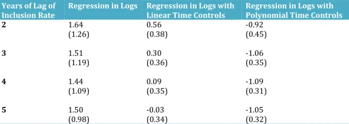
Table 21 Differences between Top Marginal Tax Rates for Dividends and Capital Gains by Country

50

Table 22 Regression in Levels of Net Migration from Norway to Sweden on the Difference in Top Tax Rates and Almon Distributed Lag Technique

57

Table 23 Responsiveness of Net Migration from Norway to Sweden to the Difference in Top Tax Rates – Period of 5 Years

58

Table 24 Regression in Levels of Total Migration from Norway to Sweden on the Difference in Top Tax Rates and Almon Distributed Lag Technique

59

Table 25 Responsiveness of Immigration from Norway to Sweden to the Difference in Top Tax Rates Period of 5 Years

60

Table 26 Regression in Levels of Total Migration from Sweden to Norway on the Difference in Top Tax Rates and Almon Distributed Lag Technique

61

Table 27 Responsiveness of Emigration from Sweden to Norway to the Difference in Top Tax Rates Period of 5 Years

62

Table 28 Responsiveness of Migration from Sweden to Norway to the Difference in Top Tax Rates P-Values for Null Hypothesis: No Impact During a 5 Year Period

63

Table A1 Reference Totals and Percentage Changes for Total Amounts of Investments Received Nationally and Inflation - Canada

76

Table A2 Migration Rates between Nordic Countries 78

Table A3 Marginal Tax Rates across Nordic Countries 80

(6)

v

INDEX OF FIGURES

Figure 1 Maximum and Minimum Percentages of Potential Revenue Gains Lost to Behavioural Responses

13

Figure 2 Percentages of Potential Increases in Revenue Lost to Behavioural Responses for Various Values of the Elasticity of Taxable Income

16

Figure 3 Potential Revenue Lost to Behavioral Responses & Estimates of Laffer Rates – Canada

17

Figure 4 Potential Revenue Lost to Behavioral Responses & Estimates of Laffer Rates – Germany

17

Figure 5 Potential Revenue Lost to Behavioral Responses & Estimates of Laffer Rates – Sweden

18

Figure 6 Comparison of Potential Revenue Lost to Behavioral Reactions across Countries

19

Figure 7 Comparison of Laffer Rates across Countries 21

Figure 8 Comparison of Laffer Rates across Countries - Restriction to Higher Values of the E.T.I

22

Figure 9 Laffer Curves for Various Values of the E.T.I. – Canada 23 Figure 10 Comparison of Laffer Curves across Countries - E.T.I. = 0.2 23 Figure 11 Comparison of Laffer Curves across Countries - E.T.I. = 0.4 24 Figure 12 Comparison of Laffer Curves across Countries - E.T.I. = 0.6 24 Figure 13 Potential Revenue Lost to Behavioral Responses & Estimates of Laffer

Rates – Chile

28

Figure 14 Potential Revenue Lost to Behavioral Responses & Estimates of Laffer Rates – Finland

30

Figure 15 Potential Revenue Lost to Behavioral Responses & Estimates of Laffer Rates - New Zealand 1990

32

Figure 16 Comparison of Potential Revenue Lost to Behavioral Reactions across Countries (Including Extrapolations)

32

Figure 17 Comparison of Laffer Rates Across Countries - Restriction to Higher Values of the E.T.I. (Including Extrapolations)

(7)

vi

Figure 18 Laffer Curves for Various Values of the E.T.I. – Chile 34 Figure 19

Comparison of Laffer Curves across Countries -

E.T.I. = 0.2 (Including

Extrapolations)

35

Figure 20

Comparison of Laffer Curves across Countries -

E.T.I. = 0.6 (Including Extrapolations)

35

Figure 21 Capital Gains Realizations and the Value of the Stock Market (Nominal Values)

42

Figure 22 Capital Gains Realizations and the Value of the Stock Market (Real Values)

42

Figure 23 National Capital Gains Realisations and Top Federal M.T.R. on Capital Gains

43

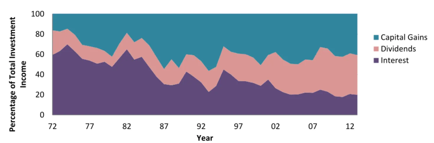
Figure 24 Stacked Breakdown of Components of Investment Income (Nominal Terms)

44

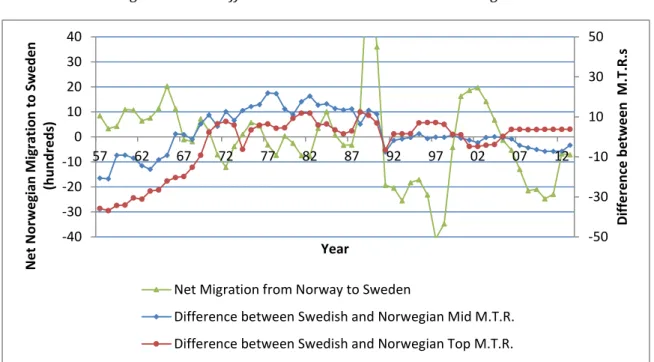
Figure 25 Stacked Breakdown of Components of Investment Income (Real Terms) 44 Figure 26 Components of Investment Income in Percentages of Total 45 Figure 27 Swedish Marginal Tax Rates and Net Nordic Migration 53 Figure 28 Migration and Differences between Swedish and Norwegian Tax Rates 54 Figure 29 Migration and Differences between Swedish and Norwegian GDP Growth

Rates

54

Figure 30 Nordic Immigration to Sweden 55

(8)

vii

List of Abbreviations

A.G.I. Adjusted Gross Income

C.A.N.S.I.M. Canadian Socio Economic Information Management System C.A.S.E.N. Encuesta de Caracterización Nacional (National Characteristics Survey)

C.D.F. Cumulative Distribution Function

C.G.R. Capital Gains Realized

E.M.T.R. Effective Marginal Tax Rate

E.T.I. Elasticity of Taxable Income

E.U. European Union

G.D.P. Gross Domestic Product

M.T.R. Marginal Tax Rate

N.W. Newey-West

N.Z. New Zealand

O.E.C.D. Organization for Economic Cooperation and Development

S.U.R.E. Seemingly Unrelated Regression

(9)

viii

REMERCIEMENTS

I would like to first thank my supervisor Prof. William McCausland for his help and guidance throughout this project. He has been a wonderful advisor, with very constructive comments.

Joshua Lewis, Norman Ferns and Feras Belabbas have made extremely useful contributions, either via discussions, helping me track down data, or both.

Prof. Fred Campano’s assistance with income distributions and computerized integration methods was invaluable.

Lastly and most importantly, my most heartfelt appreciation to my wife Silvia for her support and patience during all of my post-graduate studies.

(10)

1

1. INTRODUCTION

A central question in the implementation of government programs is financing.

A substantial part of revenue raised by most national and subnational governments in the Organization for Economic Cooperation and Development (O.E.C.D.) is through income tax. Hence taxes are not only a part of fiscal policy via their direct effects on the economy. They also underline all spending considerations. Governments must decide not only which tax rates to set, but also how many deductions to allow, and how to balance personal, corporate, payroll and sales taxes.

In terms of personal income taxes, one of the most important considerations is marginal tax rates – the percentage that the government will keep of the next dollar earned by an individual. A simplistic model for calculating changes in government revenue is to multiply the average individual’s amount of income subject to the tax increase by the number of individual tax payers, and to multiply the result by the percentage point change in the marginal rate being implemented. Yet such a calculation would almost certainly be erroneous because it assumes away behavioural responses. Individuals declare income subject to taxation and have a variety of possibilities to adjust such amounts - via working less, taking greater advantage of deductions and exemptions, controlling the timing of compensation, or engaging in illegal tax evasion. Retirement and residency decisions may also be adjusted due to tax considerations. Hence income declared will likely fall when taxes are raised, and rise when tax rates are cut.

How revenue forecasting can take such behavioural factors into account is essential in the elaboration of accurate budgets, yet doing so effectively is extremely difficult.

Although a large body of work exists on the case of the United States, the rest of the world has been examined in far less detail. This thesis seeks to fill part of that gap, by looking at prospects for raising government revenue in Canada, Denmark, France, Germany, New Zealand, Norway, Spain, Sweden, Switzerland and the United Kingdom. Alternative techniques are used to make inferences about Chile and Finland, where the detail of data is more limited.

This thesis proceeds as follows: Section 2 reviews previous literature on government revenue estimation and the responsiveness of declared taxable income to changes in marginal tax rates. Section 3 combines measures of such responsiveness with other country-specific data to estimate how government revenue can be expected to change following adjustments to top tax rates. Section 4 experiments with parametric approximations as substitutes for empirical data on income distributions for countries where these are lacking.

Finally, popular methods for estimating behavioural responses to changes in taxation rates are scrutinized. Section 5 examines the bias in estimates of taxable income responses to changes in tax rates introduced by the omission of capital gains from measures of taxable income, a practice widespread in the literature. Section 6 investigates the bias in estimates of such responses caused by not accounting for migration responses, another simplifying technique widely used. Section 7 concludes.

(11)

2

My findings are that parametric estimation methods of income distributions often work quite well and that the omission of capital gains from measures of taxable income may introduce substantial bias to published results. However, I find no evidence of substantial migration responses to changes in top marginal tax rates.

A recurring theme which is highlighted throughout this thesis is that governments are able to significantly influence how responsive taxable income is to changes in tax rates by way of availability of deductions and ease of tax avoidance. This in turn heavily impacts the amount of revenue collected.

(12)

3

2. LITERATURE REVIEW

A) An Equation for Estimating Changes in Government Revenue via Changes in Marginal Tax Rates

Saez (2004) proposes a decomposition which predicts changes in government revenue in a single year following a change to the top marginal tax rate. Thus only income which is taxed at the top marginal rate is examined. Whether changes to income at the extensive margin (i.e. retirement decisions and migration decisions) are incorporated is discussed shortly.

The equation is:

Δrevenue = N • ΔEMTR • (z – ż) • {1 – ETI • [z/(z – ż)] • [EMTR/(1 – EMTR)]}

Here, N is the number of taxpayers in the top marginal rate bracket (which is held constant as a simplifying assumption) and EMTR is the effective marginal tax rate, or the portion of an extra dollar of gross income which will be paid to the government. z is the average taxable income for those in the top rate bracket, and ż is the level of taxable income where the top tax rate kicks in. Finally, ETI is the elasticity of taxable income for those in the top tax bracket.

The E.T.I. is defined as the percentage change in reported taxable income for the average individual in the top income tax bracket when the marginal personal of-tax rate increases by 1%. The net-of-tax rate is in turn defined as 1 - (effective marginal tax rate), or as the amount of the next dollar earned which the taxpayer will be able to retain.

Intuitively, the E.T.I. is simply a measure of the response of declared taxable income to changes in the portion of additional gross income that an individual keeps.

It is noteworthy that equation (1) can be decomposed into a mechanical component (the term just to the left of the main parentheses) and a behavioural term (the part subtracted from 1 within the main parentheses). The mechanical response is what the change to government revenue would be if the E.T.I. were zero, which is to say that taxpayers would not adjust their taxable income when marginal tax rates change. The behavioural response incorporates adjustments of taxable income into revenue forecasting.

Looking more closely at the behavioural response

{ETI • [z/(z – ż)] • [EMTR/(1 – EMTR)]}

(2)

we see that this term effectively skews the true measure of change in revenue from that of the strict mechanical response. This can either lower increases in revenue or turn them into losses depending on the magnitude of the E.T.I. term.

(13)

4

Examining the effects of the country-specific variables in detail, it is clear that increases in average taxable income and decreases in the level of income where the top tax rate kicks in will raise the mechanical change in revenue collected.

In terms of behavioural responses, using algebraic analysis we can see that all else held constant, increases in the E.T.I. will increase behavioural responses. This is also true for the E.M.T.R. and the income threshold for where the top marginal tax rate kicks in. The opposite is true of the level of average taxable income of those in the top tax bracket.

Hence we see that raising the average taxable income of those in the top tax bracket will unambiguously cause government revenues to increase at a faster rate. The same is true for policies that cause the E.T.I. to fall. As the E.M.T.R. increases, the rate of increase in government revenue will fall, with government revenue falling if equation (2) exceeds zero.

Finally, the situation becomes ambiguous for changes to the income level where the top marginal tax rate takes effect. Decreases in this variable cause both the mechanical and behavioural terms in equation (1) to increase, and so the net effect on the change in revenue collected following a decrease in ż can only be determined by taking into account the values of all the variables in the equation.

Revenue is maximized when equation (2) equals 1, which is to say that raising the marginal tax rate further will cause revenue to fall.

Such a revenue-maximizing E.M.T.R. is referred to as the Laffer rate. A Laffer response is defined as tax hikes causing government revenue to fall due to the E.M.T.R. being above the Laffer rate. A Laffer curve is a graphical representation of the relationship between E.M.T.R.s and total government revenue.

(14)

5

Giertz (2009) uses equation (1) to estimate revenue-raising prospects for the U.S. Table 1 reproduces his results:

Table 1

Consequences of Various Values of the Elasticity of Taxable Income on American Taxation Policy Top Marginal Taxation Rate Bracket – 2005

(As Calculated by Giertz (2009)) Elasticity of Taxable

Income

Percentage of Potential Revenue Gains Lost to Behavioural Responses

Laffer Rate 0 0.00 1.000 0.2 24.55 0.775 0.4 49.13 0.634 0.6 73.56 0.536 0.8 98.06 0.464 1 122.53 0.410

E.M.T.R. for Top Income Bracket in 2005: 0.407 Income cut-off for top marginal rate: $326,451

Average income of those in the top marginal tax bracket: $740,481

An increase in the E.T.I. of just 0.2 is associated with an additional 12 to 24 percentage points of expected revenue gains lost to behavioral responses. The Laffer rate falls very quickly as the E.T.I. rises, by as much as 22.5 points for a 0.2 increase in the E.T.I.

B) The Challenges of Estimating the Elasticity of Taxable Income

Returning to the characteristics of the E.T.I., there are several important points which should be considered.

Generally, E.T.I.s are estimated for the short to medium term, as identification is extremely difficult in the long term due to a plethora of factors which could confound the results. These range from recessions to changes in the economic outlook for specific industries, as well as time-varying impacts of control variables in the regression equation for the E.T.I. (Saez, Slemrod & Giertz (2012)). This however imposes limitations on the accuracy of estimates for the present value of future revenue when looking at the long term. We therefore need to recognize that present abilities to forecast revenue are restricted to the medium term at best.

Lindsey (1987) provided a modern introduction to E.T.I.s, with Feldstein (1995) popularizing the topic further. Their estimates were very high compared to more contemporary findings, in the range of 1 to 3 for the general population, implying that the U.S. was on the wrong side of the Laffer curve.

Lindsey’s approach was to use repeated cross sections of taxpayers to predict what income distributions would have been like in 1982 had the tax schedule remained the same as in 1979. He then associated any deviations from the predicted income distribution as being due to behavioural responses to the tax reforms of 1981.

(15)

6

Feldstein was the first to estimate the E.T.I. using traditional panel data. This involved a collection of 4000 non-stratified, randomly selected tax returns he obtained from the I.R.S. for the years around the tax reduction of 1986. His high estimates were largely driven by the reactions of the 57 taxpayers in his sample who were subject to the highest marginal rates of 1985, and whose taxable income varied significantly over the period studied. Whether reliable inferences about large groups of taxpayers can be made from the behavioural responses of 57 individuals is not clear.

In addition to the small number of high-income taxpayers in the sample used by Feldstein, his estimation method was called into question for several reasons that also concerned the work of Lindsey (1987):

First is mean reversion, which applies at the individual level. Those with very high incomes are much more likely to experience significant reductions in earnings in the future which are unrelated to taxation. Life cycle issues (average incomes peak at a certain age before declining) also fit into this category. Without proper controls this would bias the estimates of E.T.I.s downward for tax reductions, and upward for tax increases (Auten & Carroll (1999)).

Second, those at the top of the income distribution have on average been experiencing faster increases in their income than have the rest of the population, both in nominal terms and in percentages. This is almost certainly due to factors other than income tax. Without controlling for such factors, E.T.I. estimates will be biased upward for tax cuts and downward for tax hikes.

Although the sign of the bias due to high income trends is the opposite to that of mean reversion, there is no reason to believe that the two factors will cancel (Saez (2004)).

Endogeneity of the net-of-tax rate also arises, a case of simultaneous equations. Due to the federal tax system’s progressivity, marginal tax rates increase with income. Assuming that the true value of the E.T.I. is not zero, we therefore have correlation of the explanatory variable with the error term. In order to isolate the impact of taxes on taxable income, tax rates should be imputed based on an instrumented measure of taxable income. Auten & Carroll (1999) proposed as an instrument the predicted change in net-of-tax rates assuming that inflation-adjusted income remains the same as in the base year.

Higher income groups often have more opportunities to control their taxable income. This is through choosing methods of compensation (personal income vs. corporate income, salary vs. equity), or choosing the timing of compensation (delaying being paid until after a reduction in marginal rates, and advancing their pay in anticipation of an increase in marginal rates). Hence it has been commonly proposed that the E.T.I. varies by income bracket, with the highest values corresponding to the highest earners (Gruber & Saez (2002), among many others).

The solution of Auten & Carroll (1999) for mean reversion and income share trends was to include a control for base-year income, using differencing to eliminate bias from time-constant omitted variables.

(16)

7

Their results were drastically lower than Lindsey (1987) and Feltstein (1995), with an E.T.I. estimate of 0.55 for the population as a whole.

Feldstein (1995) and Auten & Carroll (1999) excluded capital gains from their definition of taxable income, a technique which has been repeated in most studies on the matter since. However, it is not clear whether the assigned marginal tax rates used are those that would apply to the level of income with or without capital gains, with Feldstein (1995) and Auten & Carroll (1999) not addressing this point explicitly. Auten & Carroll in particular argued that those with high proportions of capital gains in their income are required to file using Alternative Minimum Tax calculations. Since data on such individuals are not generally available in panel form, they posited that such an omission from taxable income should not have a significant impact on results obtained from commonly-used panel data sets.

We should also attempt to control for the personal tax base, which is defined as the portion of national income which is subject to personal taxation. This is embodied by the availability of deductions on tax returns. More deductions result in a narrower tax base.

Changes to marginal tax rates are often accompanied by changes to said tax base. Tax cuts may be justified by an accompanying elimination of deductions in an effort to make the reduction in rates revenue neutral. Tax hikes may be accompanied by extra deductions in an effort to reduce the impact of the increases on certain groups. Thus isolating the effects of marginal tax rates on declared income is challenging (Slemrod & Kopczuk (2002)).

Kopczuk (2005) argues that with a very broad tax base the E.T.I. for even the highest income bracket is only about 0.17, roughly a third of previously accepted estimates. He does this by including the fraction of income subject to taxation as a control variable for tax bases. This micro- level variable is thus far the strongest attempt at finding a proxy to control for the macro-level tax base.

The results of Kopczuk (2005) show that the E.T.I. is influenced by policy. Hence governments can reduce its value by eliminating deductions and thereby broadening the tax base.

Turning to illegal tax evasion, Chetty (2009b) develops a utility maximization model for agents incorporating engagement in illegal sheltering activities. He concludes that governments have a large amount of control over the impacts of tax evasion. His model shows that the marginal revenue lost to increased tax evasion can on average be exactly recuperated via optimal audits. For this to hold, a risk neutrality assumption for taxpayers is required. The point stressed is that estimates of revenue lost to increases in marginal tax rates do not include revenue later recuperated in audit.

(17)

8

Chetty (2009c) demonstrates that taxpayers’ reactions to large rate changes are relatively much larger than to small rate changes. The implication is that elasticity estimates based on small rate changes will be much lower than those based on larger changes.

Classical theory predicts bunching at the kink points in the taxation structure, defined as the limit before a new tax rate kicks in. We should therefore observe evidence of behavioural responses via bunching. Saez (2010) finds evidence of this mainly in terms of cut-off rates for the earned employment refundable tax credit, a reaction concentrated among the self-employed. There is also a certain amount of bunching at the level of income where taxation starts. Quite surprisingly, he finds no evidence of bunching at any other kink points. Bastani & Selin (2011) find similar results for Sweden.

Further to these developments, Le Maire & Schjerning (2012) use Danish data to show that the self-employed retain earnings in their companies, keeping their taxable income just below the cut-offs to avoid entering another income tax bracket. In fact, of an overall estimated E.T.I. of 0.5 for the self-employed, only 0.14 to 0.2 is structural. The rest of the reaction is simply income shifting (or smoothing) from one year to another. Taxpayers who do not have self-employment income do not exhibit bunching behaviour in these results.

Through all of these results, we see that the more opportunities for tax evasion (legal or otherwise), the higher the value of the E.T.I., further reinforcing the findings of Kopczuk (2005).

C) Responsiveness of Capital Gains Realizations to Changes in Tax Rates

Of the quite limited work in this area, Auerbach (1988) uses time series data to establish that there are significant short run elasticities of reported capital gains to changes in the taxation thereof. However, estimates of permanent behavioral responses were not statistically different from zero. Auerbach, Burman & Siegal (1997) use panel data to show that long run elasticities of capital gains realisations to net-of-tax rates for capital gains are indeed very low, with little avoidance behaviour aside from temporal shifting of the realisations themselves.

Section 5 of this thesis undertakes further research on this topic.

D) Migration and Evidence of Behavioural Responses at the Extensive Margin

Despite the large majority of E.T.I. research focusing on the U.S., there has been relatively little research on state marginal tax rates and their effects on migration between states, with even less on migration between countries. However, progress has been made in certain areas.

The earliest published work is that of Feldstein & Valiant (1994), who posit that states cannot redistribute income via state income taxes. This is since taxpayers can move between states. Their conclusion has, however, been contradicted by empirical research over the years.

(18)

9

Knapp, White & Clark (2001) use a nested logit model to find that higher state income tax rates decrease emigration rates. They explain this as income taxes being a proxy for public services. However, income brackets are not differentiated, so it could be that only the residence decisions of the very wealthy are affected by state income tax rates. Such a result could be hidden by an offsetting number of people moving to the state to take advantage of better public services as the very high income earners leave. Net in-migration would show as positive under such circumstances.

Bahl, Martinez-Vazquez, & Wallace (2002) go on to find evidence that states with higher tax rates tend to have higher salaries, which could also help explain the surprising results of Knapp et al. Bakija & Slemrod (2004) look at the migration induced by state level estate taxes, and although a small correlation is found, it is not large enough to significantly impact revenue levels.

Conway & Houtenville (1998, 2001) show a negative causal relationship of marginal tax rates on net state migration of the elderly. However, Conway & Rork (2005) argue that the causal effect is more likely to be the other way around. States with influxes of seniors tend to adjust fiscal policy to accommodate them. This result is found through time variability in migration patterns and estate taxes, with the young as a control group. There could however be a causal effect of estate taxes on the migration rates of the very rich elderly.

Coomes & Hoyt (2008) examine the effects of state income tax rates on those living in metropolitan areas that span at least two states. Oddly, marginal net-of-state-tax rates have an impact on net migration rates only in states that decide residence based on state of employment (so-called states without reciprocity, which include such metropolitan areas as Chattanooga, Kansas City, Memphis, New York, Philadelphia, and St. Louis). They hypothesize that this is because there is a larger difference in state tax rates between states without reciprocity. The percentage increase in net migration to a 1% change in net-of-tax rates is estimated to be around 0.4% for those living in multi-state spanning metropolitan areas in states without reciprocity. They further estimate that a 1% increase in sales taxes is estimated to reduce net migration to the state by 0.35%.

Bruce, Fox & Lang (2010) find evidence of inter-state transferring of income, but this is done via trusts (a common financial instrument allowing income to be taxed in another jurisdiction) and not migration. This is seen through differences in federal adjusted gross income and calculated tax bases at the state level, since income received through a trust appears on tax returns at the federal level, but not on the return of the state of residence.

Young & Varner (2011) numerically estimate the elasticity of migration to state income tax rates by examining the introduction of a ‘millionaire tax’ in New Jersey. That is, the percent change in net migration of the wealthy to New Jersey following a 1% change in their net-of-state-tax rate. Their estimates are in the order of 0.1.

(19)

10

Looking at Canadian data, Day & Winer (2006) examine the effects of provincial tax rates on migration between provinces, and find very little evidence of a causal effect. Factors such as economic and (in the case of Quebec) political situations are by far the most important factors. As with many such studies, they do not differentiate between income brackets. So again, it could be that only the highest income individuals, a very small percentage of the population, are influenced to a significant degree by tax rates when choosing their province of residence.

Milligan & Smart (2013, 2014) find evidence of income shifting between provinces as a reaction to provincial tax rates, but as with Bruce, Fox & Lang (2010) this is mostly done through trusts, and not physically moving.

Kirchgassner & Pommerehne (1996) and Liebig, Puhani & Sousa-Poza (2006) study internal migration in Switzerland and its reaction to tax rates at the canton level, and find very little evidence of substantial sensitivity. They do however find evidence of migration by young, college educated citizens. These results are stated to be too small to significantly impact revenue collection. The study does not comment on the long term fiscal implications of canton-level migration of the young, however.

Kleven, Landais, Saez & Schultz (2014) find highly elastic responses of very skilled immigrants to Denmark to reductions in tax rates of recently arrived, highly skilled workers. Their estimates are of the order of 1.5 to 2.

The first paper to deal directly with inter-country migration caused by marginal tax rates is Sanandaji (2012), who uses information publicly available in Forbes to examine the migration behaviour of billionaires. He finds that the main circumstances of migration of the super-rich are to go from a poor country to a richer one, and to move to countries with political and cultural ties. However, he finds that most billionaires stay in their home countries, with taxes having a minor impact on their choices of residence. A caveat is that he only examines physical migration, and not the flight of capital.

Finally, Kleven, Landais & Saez (2013) study the migration of European soccer players between leagues and its correlation with net-of-tax rates. Interestingly, the vast majority of players choose to play in their own countries, with little impact from local fiscal policy. The exception is more skilled (and highly paid) players, who show very high elasticities of migration to net-of-tax rates of approximately 1, compared to 0.15 for domestic players.

(20)

11

3. PREDICTING GOVERNMENT REVENUE

A) Data Necessary for Estimates of Revenue Lost to Behavioural Responses

In order to apply equation (1) to estimate government revenue responses to changes in marginal tax rates, we need estimates of five different parameters.

The E.T.I. is the most challenging parameter on which to obtain data. The best source is the large volume of articles which have been written specifically to estimate E.T.I.s for a variety of countries. However, the techniques used by the authors vary considerably, with some being more rigorous than others. Most follow one of the three popular regression models outlined in the appendix. The specifics of various estimates of the E.T.I. for a variety of countries are summarized in table 3. After obtaining estimates for the E.T.I. for each country of interest, the other pieces of data necessary to apply equation (1) are values for EMTR, z (the average income of those in the top marginal tax rate bracket), ż (the income cut-off to be subject to the top marginal tax rate) and N (the number of taxpayers facing the top marginal tax rate).

Data on E.M.T.R.s are available directly from table I.7 of the tax database of the O.E.C.D., as are values for cut-offs to be in the top marginal tax bracket.

Getting estimates of average incomes for those in the top bracket and the number of people subject to the top rate is trickier. The closest data available generally come from the World Top Incomes Database (W.T.I.D.). It contains values for the cut-offs to be in the top 10, 5, 1, 0.5, 0.1 and 0.01 percent of income earners for a variety of countries. It also contains average incomes for each of these brackets.

The first step to obtain estimates of z and N is finding the percentage of top income earners corresponding to the group which is subjected to the top marginal tax rate.

After choosing the percentile whose cut-off is closest to that of the top marginal tax rate from among the income percentiles available on the W.T.I.D., I construct a quadratic interpolation. The other points are the next higher and lower percentiles for which data are available from the W.T.I.D, along with their income cut-offs.

The corresponding quadratic equation gives us an estimate of the percentage of the population subject to the top tax rate. Multiplying by the population gives the estimate of N.

A similar process, but with average incomes in place of income cut-offs, gives an estimate of z. An exception to this is for New Zealand, where the level of detail of data available from Statistics New Zealand permits direct calculation of N and z.

(21)

12

The year of most current data varies by country in the W.T.I.D. Table 2 summarizes this, and shows corresponding E.M.T.R.s and other fiscal data.

Table 2

Comparison of Fiscal Data Available from the W.T.I.D. across O.E.C.D. Countries

Country Year of Most

Current Demographic

Data

Highest Effective Marginal Tax Rate in That Year

Average Income in the Top Tax Bracket ($U.S.)*

Income Cut-Off to Enter the Top Tax Bracket ($U.S.)* Canada 2010 0.464 207,441.80 105,477.06 Denmark 2010 0.561 82,323.92

53,343.07

France 2004 0.550 154,279.22 88,229.96 Germany 2008 0.475 884,765.8 313,188.66 New Zealand** 2012 0.380 79,903.34 47,614.80 Norway 2011 0.478 155,511.92 87,437.44 Spain 2012 0.520 972,069.83 443,849.92 Sweden 2013 0.567 107,306.09 67,821.9 Switzerland 2010 0.414 370,067.60 180,350.72 United Kingdom 2012 0.520 478,831.64 215,753.79

*Dollar figures are adjusted for purchasing price parity ** Data comes from Statistics New Zealand

(22)

13 B) Results

The results suggest that even small differences in the estimated values of E.T.I.s can have enormous impacts on lost revenue. Combining published E.T.I. estimates with the tax situation at the time of the policy change studied, maximum and minimum values for the percentage of potential increases in revenue lost to behavioural responses following a rise in marginal tax rates are presented in figure 1:

Figure 1

Maximum and Minimum Percentages of Potential Increases in Revenue Lost to Behavioural Responses Based on Published Estimates of the Elasticity of Taxable Income

Based on these results, many countries could be on the wrong side of the Laffer curve. That is, they could raise substantial amounts of revenue by lowering tax rates. For the most extreme cases, a 1% reduction in top marginal tax rates would cause revenue collected from those in that income bracket to rise by 4%.

In table 3 on the next page, I turn to full results for potential revenue losses for each country studied, as well as corresponding Laffer rates and details of data used in the estimates.

0 50 100 150 200 250 300 350 400 450

Lowest % Potentially Lost Highest % Potentially Lost

(23)

(24)

15

References to equations in table 3 are found in the appendix.

E.T.I. estimates for countries with the highest tax rates (Denmark, Norway and Sweden) are consistently low, of the magnitude 0.05 to 0.5.

Still, the percentage of revenue lost to behavioural responses is substantial, at more than 25% for even a small E.T.I. of 0.05 in the case of Denmark.

Immediately noticeable is the large degree in variation in E.T.I. estimates, not just between countries but at times within a single country. Institutional factors such as availability of deductions, cultural attitudes towards government or degrees of enforcement such as audits should explain at least part of this difference. However, methodology issues such as the regression model and corresponding assumptions made as well as the quality of data almost certainly play a role. Specifics are presented in the appendix.

Laffer rates for such countries are often substantially above the E.M.T.R.s of the period studied, suggesting that governments had a window for raising further revenue, political and welfare considerations aside.

E.T.I. estimates vary substantially, not only across countries but at times across different studies for the same country. Different estimating methods are a likely explanation for this, each with its own assumptions and weaknesses. Common estimation methods are summarized in the first part of the appendix.

A general weakness in the data is that almost all estimates are based around tax cuts, with little done using data on tax increases. This is likely due to a global trend to lower tax rates which began in the early 1980s, the same period in which detailed data was first collected.

We see that estimates published in the last ten years have used substantially larger sample sizes, producing much more precise results. There is a general trend of high quality data becoming available across a range of European countries over the last decade.

(25)

16

Figure 2 shows the potential revenue increases lost to behavioural responses for a variety of countries for several plausible values of the E.T.I.:

Figure 2

Percentages of Potential Increases in Revenue Lost to Behavioural Responses for Various Values of the Elasticity of Taxable Income – Top Tax Brackets

Years of data as per table 2

The progression of the percentages lost relative to E.T.I.s is as expected given that such percentages are proportional to the E.T.I.

0 50 100 150 200 250 E.T.I. = 0.1 E.T.I. = 0.3 E.T.I. = 0.6

(26)

17

Figures 3 to 5 present behavioural responses and Laffer rates for Canada, Germany and Sweden. Figure 3

Potential Revenue Lost to Behavioral Responses & Estimates of Laffer Rates - Canada

Figure 4

Potential Revenue Lost to Behavioral Responses & Estimates of Laffer Rates - Germany

0 0.1 0.2 0.3 0.4 0.5 0.6 0.7 0.8 0.9 1 0.00% 50.00% 100.00% 150.00% 200.00% 250.00% 300.00% 350.00% 400.00% 0 0.1 0.2 0.3 0.4 0.5 0.6 0.7 0.8 0.9 1 Laf fer R ate In cr e ase in R e ve n u e Lo st to B e h av io u ral R e sp o n ses

Elasticity of Taxable Income

(27)

18 Figure 5

Potential Revenue Lost to Behavioral Responses & Estimates of Laffer Rates - Sweden

Although the percentage of mechanical revenue gains which are lost to behavioral responses varies greatly across countries, the Laffer rates are more consistent.

Further algebraic analysis of equation (1) shows that changes in N have no effect on the relationship between the E.T.I. and the percentage of increases in revenue lost to behavioral responses:

Δrevenue = N • ΔEMTR • (z – ż) • {1 – ETI • [z/(z – ż)] • [EMTR/(1 – EMTR)]}

We have that

i) N • ΔEMTR • (z – ż) is the mechanical revenue response

ii) N • ΔEMTR • (z – ż) • ETI • [z/(z – ż)] • [EMTR/(1 – EMTR)] is the behavioral response

or the amount of potential revenue lost.

iii) Therefore the percentage of revenue gains lost to behavioral responses is simply ii/i, or ETI • [z/(z – ż)] • [EMTR/(1 – EMTR)]. N does not appear.

iv) Finally, [z/(z – ż)] • [EMTR/(1 – EMTR)] is the slope of the blue lines in figures 2 to 4.

As the E.M.T.R. gets larger, the slope of the line corresponding to percentage revenue gains lost for a given value of the E.T.I. gets steeper. This is also true for decreases in z and increases in ż.

(28)

19

Hence for a given value of the E.T.I., countries that have higher percentages of potential revenue gains lost to behavioral responses either have a higher E.M.T.R., a lower average income for those in the top tax bracket, or a higher cut-off to be in the top income tax bracket. Raising average income for those in the top tax bracket will raise government revenue by increasing potential revenue to be collected. The percentage of revenue lost to behavioral responses will fall. The situation is similar when lowering the cut-off to be in the top tax bracket.

We can see these effects visually in figure 6 for a choice of 4 countries with noticeable differences in the percentages of revenue lost to behavioral responses:

Figure 6

Comparison of Potential Revenue Lost to Behavioral Reactions across Countries

Following the above the discussion, it is clear that the driving forces behind the variations across countries comes from differences in marginal tax rates, average incomes in the top tax bracket, and the level of income where the top marginal tax rate kicks in. Quantifying how much of the variation is due to each of these factors is more challenging.

A natural strategy would be to take partial derivatives of equation (2) with respect to each variable of interest. However, this strategy is confounded by the average income of those in the top tax bracket being dependent on the income cutoff to be in the top tax bracket. The higher the cut-off, the higher the average income of those left in that group. Unfortunately, the relationship between these factors is very difficult to measure without having the exact shape of the income distribution for the country in question. Making further approximations to get around this issue could lead to false inferences about which factors have the most impact.

0% 50% 100% 150% 200% 250% 300% 350% 400% 0 0.1 0.2 0.3 0.4 0.5 0.6 0.7 0.8 0.9 1 In cr e ase in R e ve n u e Lo st to B e h av io u ral R e sp o n ses s

Canada Denmark Sweden Switzerland

(29)

20

It is perhaps preferable to simply assume that the two are independent, which should be approximately true in small neighbourhoods around the observed values.

Table 4 presents partial derivatives evaluated at the most current data points available for the four countries of figure 5, without considering the E.T.I.:

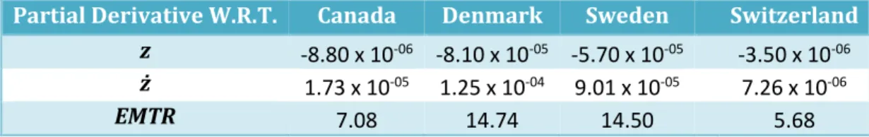
Table 4

Partial Derivatives of the Equation for Percentage of Revenue Lost to Behavioural Responses Taken With Respect to Its Influencing Factors

Evaluated at Most Current Values of Each Variable

Partial Derivative W.R.T. Canada Denmark Sweden Switzerland

z _{-8.80 x 10}-06_{-8.10 x 10}-05_{-5.70 x 10}-05 _{-3.50 x 10}-06

ż _{1.73 x 10}-05 _{1.25 x 10}-04 _{9.01 x 10}-05 _{7.26 x 10}-06

EMTR _7.08 _14.74 _14.50 _5.68

We see that generally, the values for all partial derivatives are higher for Denmark and Sweden than for Canada and Switzerland. The values for the partial derivatives w.r.t. z and ż are easily comparable, as they are of the same units. However, it is not obvious how to compare them to the values w.r.t. the EMTR.

Table 5 makes an attempt in this sense by examining ratios: Table 5

Ratios of Partial Derivatives of the Equation for Percentage of Revenue Lost to Behavioural Responses Taken With Respect to Its Influencing Factors

Evaluated at Most Current Values of Each Variable Canada Denmark Sweden Switzerland

ż/z _-1.97 _-1.54 _-1.58 _-2.05

EMTR/z -806316 -181607 -254452 -1604616

EMTR/ ż 409984 117674 160824 782002

Here we see that in Denmark and Sweden the effective marginal tax rate and income cut-offs for the top tax bracket exert much less influence on the percentage of revenue lost to behavioural responses relative to the average income of those in the top tax bracket. Hence we can expect that the lower average incomes of those in the top tax bracket in Denmark and Sweden relative to other countries is what drives their potential for large percentages of income lost to behavioural responses.

(30)

21

An equation for the Laffer rate is

1/{[(z•ETI)/(z- ż)]+1}.

(3) From this, we can see that decreasing the E.T.I., decreasing the cut-off to be in the highest income tax bracket, or increasing the average income of those in the top marginal tax bracket will raise the Laffer rate. Hence we expect those countries with the highest Laffer rates to have the lowest E.T.I., lowest cut-off for the top income tax bracket, or highest average income for those in that bracket. Countries with the highest tax rates such as Denmark and Sweden have the lowest Laffer rates, with Sweden’s being 0.2690 for an E.T.I. of 1. This implies that the Scandinavian model of high tax rates and a wide variety of services is dependent on low E.T.I.s to function.

Figures 7 and 8 present a visual representation of Laffer rates: Figure 7

Comparison of Laffer Rates across Countries

0.2 0.3 0.4 0.5 0.6 0.7 0.8 0.9 1 0 0.1 0.2 0.3 0.4 0.5 0.6 0.7 0.8 0.9 1 Laf fer R ate

Canada Denmark Sweden

(31)

22 Figure 8

Comparison of Laffer Rates across Countries Restriction to Higher Values of the E.T.I

This section concludes with a collection of Laffer curves showing how total revenue collected from the top tax bracket changes with the top marginal tax rate under several different values of the E.T.I.

Since for E.T.I. = 0 we simply have the mechanical component of the increase in revenue from a change in top marginal tax rates, such Laffer curve are always linear.

For positive values of the E.T.I., the Laffer curve becomes the standard hill, although it is somewhat skewed to the right. It gets flatter and lower for higher values of the E.T.I., and the top of the curve, corresponding to the Laffer rate, moves to the left and is reached at a lower E.M.T.R.

0.25 0.27 0.29 0.31 0.33 0.35 0.37 0.39 0.41 0.43 0.45 0.7 0.8 0.9 1 Laf fer R ate

(32)

23 Figure 9

Laffer Curves for Various Values of the E.T.I. - Canada

The last three figures, 10 to 12, show a direct comparison of Laffer curves across countries. By raising the Laffer rate, a country collects more tax revenue per taxpayer in the top tax bracket when measured in U.S. dollars and adjusted for purchasing power parity.

Figure 10

Comparison of Laffer Curves across Countries E.T.I. = 0.2 0.0 20.0 40.0 60.0 80.0 100.0 120.0 140.0 160.0 0 6 12 18 24 30 36 42 48 54 60 66 72 78 84 90 96 Go ve rn m e n t R e ve n u e Fr o m To p B rac ke t Taxpayer s in B ill io in s o f Can ad ai an Do llar s

Top Bracket Effective Marginal Tax Rate

E.T.I. = 0 E.T.I. = 0.2 E.T.I. = 0.4 E.T.I. = 0.6 E.T.I. = 0.8 E.T.I. = 1 0.0 20,000.0 40,000.0 60,000.0 80,000.0 100,000.0 120,000.0 140,000.0 160,000.0 0 6 12 18 24 30 36 42 48 54 60 66 72 78 84 90 96 Go ve rn m e n t R e ve n u e Per To p B rac ke t Taxpayer in U.S . Do llar s A d ju ste d fo r Pu rc h asi n g Po we r Par ie ty

(33)

24 Figure 11

Comparison of Laffer Curves across Countries E.T.I. = 0.4

Figure 12

Comparison of Laffer Curves across Countries E.T.I. = 0.6 0.0 20,000.0 40,000.0 60,000.0 80,000.0 100,000.0 120,000.0 140,000.0 160,000.0 0 6 12 18 24 30 36 42 48 54 60 66 72 78 84 90 96 Go ve rn m e n t R e ve n u e Per To p B rac ke t Taxpayer in U.S . Do llar s A d ju ste d fo r Pu rc h asi n g Po we r Par ie ty

Canada Denmark Sweden United Kingdom 0.0 20,000.0 40,000.0 60,000.0 80,000.0 100,000.0 120,000.0 140,000.0 160,000.0 0 6 12 18 24 30 36 42 48 54 60 66 72 78 84 90 96 Go ve rn m e n t R e ve n u e Per To p B rac ke t Taxpayer in U.S . Do llar s A d ju ste d fo r Pu rc h asi n g Pow e r Par ie ty

(34)

25

4. WORKING WITH LESS DETAILED DATA

A) Introduction

The results presented thus far are exclusively for high income countries.

To examine issues related to raising tax revenue for low and middle income countries, a serious difficulty is limited availability of data.

Most income data on such countries are usually in the form of average incomes or income shares by grouped percentiles. Details of income distributions necessary to perform detailed studies on revenue collection and behavioural responses are not available.

This is particularly true of the highest income individuals. Inferences about their incomes cannot be meaningfully approximated from data on average incomes per population decile. Yet high income individuals present the largest behavioural responses to taxation, and are the source of a large portion of government revenue.

Getting around these limitations would allow us to obtain very interesting results, given the lower marginal tax rates generally in place in middle and low income nations.

For instance, Hourton (2012) provides income cut-off information per decile of the population in Chile using the Encuesta de Caracterización Socioeconómica Nacional (CASEN) for 2006. This is a mandatory survey issued by the government of Chile, and is the most reliable information on household income available to academics. However, since income data is based solely on amounts reported in the survey, inaccuracies relating to reporting errors by high income households present a serious challenge.

Putting such inaccuracies aside, once we have some information on income cut-offs in the income distribution, a feasible way to make inferences about those at the top of the income distribution is to look for ways to fit known income distribution functions to the limited data available.

One example was presented in Dagum (1977). He proposed a density function as follows:

f(y) = (1-α)λβδ•y

-δ-1

_(1+λ•y

-δ

₎

-β-1_{for income y > 0 (4)}

To obtain the percentage of the population subject to the top tax rate, we use the Dagum CDF, given by:

F(y) = α + (1-α)/(1+λ•y

-δ

₎

β_{, λ > 0 (5)}

Its inverse is given by:

y = λ

1/δ

_{{[(1-α)/(p-α)]}

1/β

_-1}

1/δ

₍₆₎

(35)

26

To obtain estimates of the average income for those in the top income tax bracket, we need to integrate the inverse of the CDF. The area of integration is from the percentage of the population subject to the top income tax rate to the top of the income distribution. Numerical estimation methods for the integral present one possible way forward.

An alternative approach which is explored in this thesis is developed in Saez, Slemrod & Giertz (2012). They recognize that the right tail of an income distribution is well approximated by a Pareto distribution. This has by definition a density function of the form f(z) = C/z1+α_{. Denoting by}

zm_{the average income of those in the top bracket and ż the income level where the top marginal tax} rate kicks in, they point out that we have zm_{= ∫zf(z)dz/∫f(z)dz, where the range of both integrals is} from ż to infinity. This expression is in turn equal to ż•α/(α-1), where in the results it is no longer necessary to know the value of C. Hence, once the value of the Pareto α is known, assuming it is greater than 1 we can obtain an estimate for the average income for those in the top marginal tax bracket.

In order to obtain the required estimate of the Pareto α, we can look at a second functional form used to approximate income distributions, presented by Champernowne (1952). The density function is given by:

f(y) = (2Nασsinϴ(y/y

0

)

ѱ

/(y(1+σ)ϴ{1+2cosϴ(y/y

0

)

ѱ

+(y/y

0

)

2ѱ

})

(7)

where ѱ = α when y > y0 and ѱ = ασ otherwise.

Champernowne (1952) shows that the above parameter α converges asymptotically to the Pareto parameter α of the right tail of the income distribution in question, which is the α discussed just above. Hence, once we have an estimate of α for the Champernowne formula above, we can quickly calculate an estimate of the average income of those in the top tax bracket.

Note that the Dagum α has no direct connection to the Champernowne/Pareto α, and is designated by the same symbol by convention only.

In terms of techniques to estimate the parameters of the two income distribution functions given above, Campano (2006) provides an iterative program which selects a set of parameters for either the Dagum or Champernowne formulas so as to minimize the CHI square. The selection is taken from a collection of approximately 20,000 of the most likely combinations of such parameter values.

B) Revenue Forecasts Using Income Distribution Function Extrapolations

The goal of what follows is to investigate the potential of the Dagum, Champernowne and Pareto distributions in order to make inferences about underlying income distributions of nations that do not have a rich source of data readily available.

(36)

27 Returning to the case of Chile, we obtain the following:

Table 6

Income Distribution Results for Chile 2006

E.T.I. (Fernandez 2010) 2.0

Source of population data Hourton (2012)

Dagum α 0.011312 Dagum β 1.3582 Dagum λ 0.67674 Dagum δ 1.6586 Champernowne α 1.5897 Champernowne ϴ 0.008422 Champernowne y0 8911.3 Champernowne σ 1.2737

ż (Income cut-off for top M.T.R.) U.S. $124,100

Estimate of percentage of the population subject to top M.T.R. via Dagum C.D.F. 1.3773

N (number of people in the top tax bracket) 171,149

z (average income of those in the top tax bracket) via Pareto U.S. $334,545

z via integration of Champernowne inverse C.D.F. U.S. $311,743

Top marginal tax rate 40.00

% revenue lost to behavioural responses via Pareto distribution method 211.96 % revenue lost to behavioural responses via integration of the Champernowne

inverse C.D.F.

221.52

Laffer rate via Pareto distribution method 23.92

Laffer rate via integration of the Champernowne inverse C.D.F. 23.13

The E.T.I. estimate comes from Fernandez (2010), who also uses the CASEN for 1996 to 2006 to obtain an estimate for Chile of 2.0. It is not possible to tell how much her estimates were influenced by reporting biases in the survey, as this estimate is very high.

Included in table 6 are estimates of the average income of those in the top tax bracket via integration of the Champernowne formula’s inverse CDF function, as provided by Fred Campano. We can see that since the Pareto method may over-estimate top average incomes in this case, it provides a lower estimate of the potential percentage of revenue lost to behavioural changes. The very high income cut-off for the top tax rate relative to average incomes heightens concern about the accuracy of the survey-based data. Since this is quite a small portion of the population, reporting errors by a subset of the group could have large impacts on both the E.T.I. estimate and the calculations of lost revenue.

(37)

28

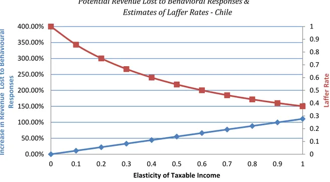
Figure 13 summarizes potential lost revenue and Laffer rates for a range of more moderate E.T.I. values:

Figure 13

Potential Revenue Lost to Behavioral Responses & Estimates of Laffer Rates - Chile

Interestingly, potential revenue lost to behavioural responses for a given value of the E.T.I. is lower than many richer nations already studied. This is at least somewhat foreseeable due to the high average incomes of those in the top tax bracket and the discussion in section 3.

I now turn to Finland as an additional example of this method. Unlike Chile, Finland does not suffer from a lack of data generally. However, Statistics Finland only releases income distribution data in tabulated form by decile. Additionally, the W.T.I.D. (which was the source of income data in section 2) lacks detailed information on this country.

Mattika (2014) uses panel data involving 550,000 tax returns per year for the period 1995 to 2007 to obtain a plausible estimate of the Finnish E.T.I. of 0.475. The data cover the entire income distribution, and he presumes that the E.T.I. is applicable to all income groups, a strong assumption found frequently in the literature.

(38)

29 Using the Pareto method, we obtain the following results:

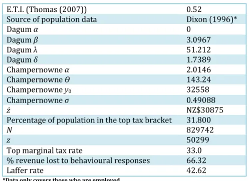
Table 7

Income Distribution Results for Finland 2007

E.T.I. (Mattika (2014)) 0.475

Source of population data Statistics Finland

Dagum α 0 Dagum β 0.87654 Dagum λ 445620 Dagum δ 4.0003 Champernowne α 4.0619 Champernowne ϴ 0.0988 Champernowne y0 25467 Champernowne σ 0.88932 ż €64,006.20

Percentage of population in the top tax bracket 2.268

N 99,610

z €84,910.28

Top marginal tax rate 56.1

% revenue lost to behavioural responses 246.56

Laffer rate 34.14

Although the top marginal tax rate in Finland is comparable to other Nordic countries, the much higher E.T.I. estimate results in a very large amount of revenue predicted to be lost to behavioural responses.

The higher value of the Pareto/Champernowne α relative to that of Chile fits with expectations that wealth inequality is not as extreme in Finland, as shown by a ‘skinnier’ right-hand tail of the income distribution.

The much smaller value of the Dagum α relative to Chile also gives less cause for concern in terms of the Dagum model’s fit of the entire income distribution. The Dagum distribution function can be expected to give meaningful inferences over very nearly the entire income distribution.

(39)

30

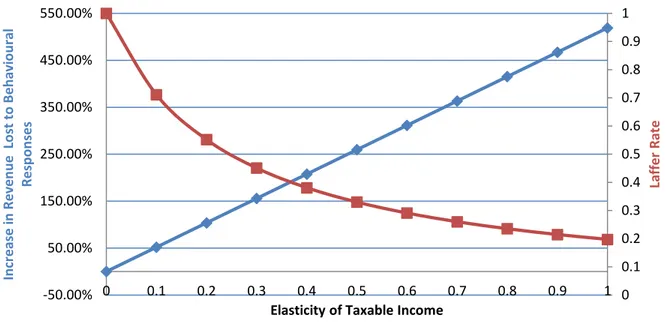
Figure 14 presents Laffer rates and lost revenue for Finland. Noteworthy are the lower Laffer rates and higher percentages of lost revenue, consequences of a lower top bracket income cut-off and lower average income in that bracket.

Figure 14

Potential Revenue Lost to Behavioral Responses & Estimates of Laffer Rates – Finland

As a third example, the tax reform of New Zealand in 1990 makes for an interesting study. At that time, the government of New Zealand instituted a tax schedule which was very nearly flat, especially in comparison to other industrialized nations. The top tax rate was set to 33%. The level of income where the top rate kicked in was NZ$30,875, or just over US$18,000.

The study of New Zealand presented in section 3 focused on a period when the country had returned to a more progressive tax structure.

Although very detailed income distribution data is made publicly available by Statistics New Zealand, these go back only to 2001. Earlier years’ data were never released.

However, Dixon (1996) uses the Household Economic Survey of New Zealand to tally income summaries for those who were working.

The Pareto distribution characteristics discussed above are assumed only to hold at the right tail of the income distribution, hence the technique is not applicable in this case. The Dagum formula predicts 31.8% of the population was subject to the top M.T.R., a group which is far from being constrained to that right-hand tail.

0 0.1 0.2 0.3 0.4 0.5 0.6 0.7 0.8 0.9 1 -50.00% 50.00% 150.00% 250.00% 350.00% 450.00% 550.00% 0 0.1 0.2 0.3 0.4 0.5 0.6 0.7 0.8 0.9 1 Laf fer R ate In cr e ase in R e ve n u e Lo st to B e h av io u ral R e sp o n ses