Demand-driven type analysis for dynamically-typed functional languages

(1)

Demand-Driven Type Analysis

for Dynamically-Typed Functional Languages

par Danny Dub´e

Département d’informatique et de recherche opérationnelle Faculté des arts et des sciences

Thèse présentée à la Faculté des études supérieures en vue de l’obtention du grade de Ph.D.

en Informatique

Aoˆut, 2002

c

(2)

Faculté des études supérieures

Cette th`ese intitul´ee:

Demand-Driven Type Analysis

for Dynamically-Typed Functional Languages

pr´esent´ee par:

Danny Dub´e

a été évaluée par un jury composé des personnes suivantes:

Gilles Brassard pr´esident-rapporteur Marc Feeley directeur de recherche Alain Tapp membre du jury Matthias Felleisen examinateur externe

Gilles Brassard (par interim) repr´esentant du doyen de la FES

(3)

R´

esum´

e

Nous présentons une nouvelle analyse de types destinée aux langages typés dynami-quement qui produit des résultats de grande qualité à un coût qui la rend utilisable en pratique. Bien que statique, l’analyse est capable de s’adapter aux besoins de l’optimiseur et aux caractéristiques du programme à compiler. Le résultat est un analyseur qui se modifie rapidement pour être en mesure de mieux effectuer son travail sur le programme. Des tests démontrent que notre approche peut user de passablement d’intelligence pour permettre la réalisation de certaines optimisations.

L’analyse est adaptable parce qu’elle est effectuée à l’aide d’un cadre d’analyse pa-ramétrisable qui peut produire des instances d’analyses à partir de modèles abstraits. Ces modèles abstraits peuvent être remplacés au cours de l’analyse du programme. Plusieurs pro-priétés du cadre d’analyse sont présentées et démontrées dans ce document. Parmi celles-ci, on retrouve la garantie de terminaison associée à toute instance d’analyse produite à l’aide du cadre, la capacité d’analyser parfaitement tout programme qui se termine sans erreur et la capacité d’imiter plusieurs analyses conventionnelles.

Les modifications apportées au modèle abstrait en fonction des besoins de l’optimiseur le sont grâce à l’utilisation de demandes et de règles de traitement des demandes. Les demandes décrivent des requêtes pour la démonstration de propriétés jugées utiles à l’optimiseur. Les règles de traitement permettent la traduction de demandes décrivant les besoins de l’optimiseur en des directives précises de modifications au modèle abstrait. Chaque directive de modification du modèle peut apporter une aide directe à l’optimiseur parce que les règles de traitement font en sorte que des demandes justifiées sont transformées en d’autres demandes justifiées.

(4)

et a été implantée. Le prototype implantant cette approche a démontré le potentiel considé-rable de nos travaux. Il faudra encore effectuer d’autres recherches avant qu’on puisse utiliser couramment notre approche dans les compilateurs. C’est toutefois compréhensible si on considère que tous nos travaux, outre les idées liées aux analyses statiques conventionnelles, sont une contribution originale.

Mots-cl´es : analyse sur demande — analyse adaptable — analyse statique — analyse de types — techniques de compilation — optimisation de programmes

(5)

Abstract

We present a new static type analysis for dynamically-typed languages that produces high quality results at a cost that remains practicable. The analysis has the ability to adapt to the needs of the optimiser and to the characteristics of the program at hand. The result is an analyser that quickly transforms itself to be better equipped to attack the program. Experiments show that our approach can be pretty clever in the optimisations that it enables.

The analysis is adaptable because it is accomplished using a parametric analysis frame-work that can instantiate analyses by building them from abstract models. The abstract models can be changed during the analysis of the program. Many properties of the analysis framework are presented and proved in the dissertation. Among which there is the guar-antee of termination of any analysis instance it produces, the capacity to analyse perfectly well error-free terminating programs, and the ability to mimic many conventional static analyses.

Modifications to the abstract model in response to the needs of the optimiser are realised through the use of demands and demand processing rules. Demands express a request for the demonstration of a property deemed useful to the optimiser. The processing rules allow demands that directly express the needs of the optimiser to be translated into precise proposals of modifications to the abstract model. Each modification to the model that is proposed is potentially directly helpful to the optimiser because the processing rules ensure that pertinent demands are translated into other pertinent demands.

A complete approach of demand-driven analysis based on pattern-matching is exposed and has been implemented. The prototype implementing the approach has demonstrated that our work has great potential. Further research has to be conducted to make the method

(6)

usable in everyday compilers. Still, this is understandable, considering that our whole work, except the notions related to conventional static analysis, is original material.

Key-words: demand-driven analysis — adaptable analysis — static analysis — type anal-ysis — compilation techniques — program optimisation

(7)

List of Tables

6.1 Experimental results . . . 176

6.2 The effect of the size of a program on the analysis . . . 178

(13)

List of Figures

2.1 Mini-language syntax . . . 15

2.2 Mini-language semantics . . . 15

3.1 Instantiation parameters of the analysis framework . . . 22

3.2 Analysis results of the framework . . . 25

3.3 Evaluation constraints . . . 32

3.4 Safety constraints . . . 37

3.5 Semantics of the collecting machine . . . 39

3.6 Function computing the set of sub-expressions . . . 40

3.7 Function computing the set of immediate sub-expressions . . . 41

5.1 Syntax of the modelling patterns . . . 96

5.2 Definition of the conformance relation . . . 97

5.3 Algorithm for the conformance relation between modelling patterns . . . . 98

5.4 Implementation of the pattern-matchers . . . 105

5.5 Algorithm for pattern-matching . . . 106

5.6 Syntax of the split patterns . . . 108

(14)

5.8 Example of simplification of a split pattern . . . 111

5.9 Generation of pattern-matcher update requests to ensure consistency . . . 111

5.10 Example of an update request and the sub-requests generated for consistency 112 5.11 Slicing of split patterns . . . 113

5.12 Example of the slicing of a split pattern . . . 113

5.13 Extension of the definition of conformance between modelling and split pat-terns . . . 114

5.14 Algorithm for the upgrade of inspection points in pattern-matchers . . . . 115

5.15 Example of the upgrade of a pattern-matcher . . . 117

5.16 Syntax of the demands . . . 118

5.17 Algorithm for the “is spread on” relation . . . 118

5.18 Definition of the “have a non-empty intersection” relation . . . 119

5.19 Definition of the intersection operator between patterns . . . 135

5.20 Example of couples to separate . . . 139

5.21 Example of a na¨ıve separation . . . 140

5.22 Example of a more clever separation . . . 140

5.23 Implementation of the Split-Couples function . . . 141

5.24 Example of computation made by Split-Couples . . . 146

5.25 Algorithm for the demand-driven analysis . . . 153

6.1 Translation of letrec-expressions . . . 171

6.2 Translation from the Scheme subset to the extended mini-language . . . . 173

(15)

Remerciements

Je tiens à remercier ma copine, Marie-Lisa. Elle a toujours été encourageante et a su m’apporter la motivation nécessaire. Merci à mes parents, ma soeur et son mari. Tous m’ont accompagné dans mon cheminement et ont constitué un milieu réconfortant durant tous les moments, heureux et pénibles.

Je tiens par-dessus tout à remercier mon directeur de thèse, Marc Feeley, pour son support, tant moral que financier et technique. Il a su être aussi patient qu’il fallait l’être avec moi. Il a toujours cru en moi, plus que je ne pouvais croire en moi-même. Il m’a toujours témoigné un grand respect, même quand j’étais une peste d’entêtement.

Merci à toute la grande famille au complet, à mes amis et à mes camarades à l’école. Tout particulièrement : Odi pour m’avoir aidé à garder la forme et dont la compagnie est toujours agréable ; Sébastien pour être M. Divertissement en personne ; Mohamad qui m’a apporté une authentique aide et avec qui j’allais noyer ma déprime dans la caféine ; Diane qui a insisté avec tellement d’énergie pour que je complète mon doctorat ; le très constant (et comique) Mario ; Dominique ; Martin ; Wissam ; Fernanda ; Éric ; Étienne et Jean-Fran¸cois qui ont été si tannants et qui ont subi mes foudres tellement souvent (“Danny, t’es pas parlable !”) ; et Fran¸cois qui m’a aidé à découvrir ma vraie nature de dictateur.

L’aide financière des organismes subventionnaires CRSNG et FCAR m’a été précieuse. Elle n’a pas été vaine, après tout.

(16)

Introduction

1.1 A Gentle Introduction

Very high quality type analysis can be performed on programs written in a dynamically-typed functional language while maintaining control over the analysis time. A quality type analysis is achieved by using a “clever” adaptive analysis method called demand-driven analysis. Although the method does not come from traditional artificial intelligence, it allows the analysis to adapt to the characteristics of the program at hand in ways that seem rather intelligent. But all this is quite vague, so let us proceed from the beginning.

Program analyses that are used for optimisation purposes are always stretched between two contradictory goals: quality and efficiency. Indeed, the user of a compiler wants the compiler to produce the best possible code while taking the least possible time to do so. Unfortunately, these desires are incompatible.

Roughly speaking, in the case of type analysis, two kinds of analyses exist, depending on which goal is considered to have priority. Fast analyses aim the efficiency of the analysis while heavy analyses aim the quality of the generated code. The fast ones feature reasonable analysis times and obtain results of a fair quality. The heavy ones inspect the program very closely and do not feature reasonable analysis times. Commonly used compilers that perform some type analysis use a fast one because the heavy ones are too costly in practice.

(17)

version is still interesting. What we are interested in is a type analysis of very high quality that can be performed within times that remain practical. In our opinion, an analysis featuring practical times is crucial if we want our type analysis or a derivative to eventually be applied in some routinely used compiler. Despite the fact that our goal is relaxed, it still seems to be a na¨ıve, “spoiled child’s” desire. It seems to disregard the apparently strong relation between quality and efficiency that years of research in type analysis have outlined. Until now, this empirical relation has brought the user to expect a certain cost for a certain quality. Our childish desire lies in the high-quality part of the spectrum while incurring a cost that is well under the one that the quality-efficiency relation suggests. Is it reasonable to aim at such a goal?

We believe it is reasonable because a small amount of cleverness often pays off more than a lot of brute force. This is so in many aspects of real life and in computer science, too. For example, during a war, the army with the greatest number of soldiers and the best equipment does not necessarily defeat its enemy if it is poorly directed. In computer science, an O(n log n) algorithm can outperform an O(n2_{) algorithm, even if the latter is}

run on a computer that is faster by orders of magnitude. However, discovering the better algorithm requires careful thought.

But what clever thing could be done about type analysis? This thesis has its origins in an innocent sounding remark by my supervisor, roughly paraphrased as: “It would be nice to have an analysis that is very powerful but that uses its power only as much as needed by the optimiser to perform its job.” We all know something that has this kind of behaviour; that is, something powerful but always trying to do as little as possible: a human. Let us imagine an optimising compiler where the type analysis would be done by a human; say, Mr. D. Let us describe the way Mr. D would proceed in analysing a program.

Mr. D would use his intelligence to perform the analysis. And he would perform a very good one. Indeed, he wants to help the compiler to produce highly optimised code. But he would use his intelligence mostly where it would really help the optimiser. That is, Mr. D is lazy. If an easy check allows the optimiser to improve a particular piece of code, Mr. D will not waste his time by making a complex proof involving the full extent of his mathematical knowledge.

The mental work performed by Mr. D can be divided in two parts: raw program analysis and reasoning about the task of analysing the program. The raw analysis part is essentially

(18)

similar to what conventional analyses do. On the other hand, he does the reasoning part by inspecting the program, by looking at the analysis results, by inventing new raw analyses, by searching for the right invariants, etc. The raw analysis part can be done by hand or by writing an algorithm and running it on a machine. It does not matter how it is done. It is mechanical work, anyway. But Mr. D is able to do the reasoning part only because he is intelligent and understands what he is doing.

To summarise Mr. D’s work, we would say that he is intelligent, he is lazy, and he knows what he is doing. He is able to analyse the program while he is also able to elaborate strategies about the way he should analyse the program. The demand-driven analysis approach that we introduce in this dissertation is inspired by the clever behaviour of Mr. D. Our approach features the same division of the work into a raw analysis part and a reasoning part. The reasoning part is able to modify the way raw analysis is done. The approach features laziness as the reasoning part is goal-driven: it takes care of the needs of the optimiser and only of these; any modification to the way raw analysis is done derives from those needs. Up to this point, our approach seems to act exactly as Mr. D. But, as expected, there is a difference and it lies in the fact that our approach does not understand what it is doing. It is only a combination of numerous deterministic algorithms and it does not exhibit any sign of learning or understanding whatsoever. Nevertheless, experiments have shown that it exhibits considerable cleverness in the execution of its task. This is satisfying as only intelligence is required, not consciousness.

1.2 Some More Precisions

The purpose of our type analysis is to help the optimiser to remove unnecessary dynamic safety type tests from the executable. The code resulting from the compilation of a program written in a dynamically-typed language includes dynamic safety type tests in the code of many primitive operations. For example, let us consider the following Scheme1 expression: (car x). This expression extracts the object in the first field of the pair contained in ‘x’, provided ‘x’ really contains a pair. Since Scheme is dynamically-typed, ‘x’ could poten-tially contain objects of any type, depending on the computations done by the program. Consequently, the ‘car’ function must perform a safety type tests before it can extract the

(19)

contents of the first field. Safety tests guarantee that the execution of the program proceeds safely.

If no test were performed before ‘car’ did the extraction, the extraction could trigger an illegal operation at the hardware or operating system level and an abnormal termination of the program would occur. Or the illegal extraction could go undetected and cause a corruption of the data of the program, leading to potentially disastrous consequences. High-level languages such as Scheme are designed with safe execution in mind. Consequently, it is natural to include such dynamic safety tests in the executable.

Of course, these safety tests incur a penalty in the efficiency of the executable program. So it is perfectly understandable to want to avoid the added inefficiency. A common way to do so consists in telling the compiler to omit the inclusion of those tests. All potentially illegal operations made by the executable program then go unchecked and result in low-level crashes or program misbehaviour in case of an error. In this work, we choose not to consider this “solution”. We prefer to insist on keeping the safety of the execution and turn to another option: safe optimisations. For some operations made by the program, the compiler may be able to determine that they can never go wrong. Safe optimisations can be enabled only in these cases. For example, the (car x) expression need not include a dynamic safety test if the compiler is able to determine that ‘x’ cannot contain anything else than pairs. The demonstrations needed to trigger safe optimisations are obtained through the use of static analysis.

But what is a static analysis? It is the gathering of informations about the execution of the program. The nature of the informations that are gathered depends on what the optimiser needs to perform its task. They may relate to the heap-space usage, the liveliness of the objects at run-time, the may-alias information, or something else. In this work, the informations that interest us is the type of the values involved in the computations done by the program. What is particular to static analyses is the method that is used to gather the informations: a phony execution of the program or some other process that does not involve its real execution. It is mandatory to avoid the real execution because its duration is unknown (and possibly infinite). On the other hand, the phony execution requires the manipulation of phony values only for a bounded number of steps. So it is fast (and predictable) enough to be a part of a compilation. The reader may find numerous examples of static analyses in [3].

(20)

Despite the fact that the static execution is phony, it is designed in such a way that it has a mathematical connection to the real execution. Consequently, the results of the phony execution constitute the desired informations about the real execution. In general, the informations are only approximations of what could be observed if the program were really run. Moreover, in order to be useful to the optimiser, these informations have to be conservative.

When we say that the gathered informations have to be conservative, it means that they must take into account at least all possible behaviours of the program. But why is it “at least” and not “at most” or “the best approximation of”? Because of the nature of typical optimisations. Optimisations, such as the removal of safety type tests, require a particular property to be true for all possible executions of the program. Consequently, if the property is true for all behaviours listed in the description, then it has to be true for all concrete behaviours of the program. For example, if the analysis says that ‘x’ can contain nothing else than pairs, then, during the concrete execution of the program, it is certain that ‘x’ contains a pair (at least, if ‘x’ ever comes to existence) and (car x) can be optimised.

In opposition to the conservativeness of the analysis results, there is the need of the optimiser for results that are as useful as possible. It is clear that obtaining a conservative analysis is easy. We only need to write an analysis that pretends that anything may happen during the execution. Note that these analysis results are certainly conservative. However, the analysis results thus produced would not be useful as the property allowing optimisations to be performed would not be true in general (according to the results). For example, if the type analysis blindly determines that ‘x’ potentially contains objects of any type (which is true), then the optimisation of (car x) cannot be performed.

Essentially, the best interest of the analyser is to overestimate the description as little as possible while it must imperatively avoid underestimating the description. Reducing the overestimation as much as possible requires increasing the computational effort put into the analysis. However, an increase in the computational effort means that the compilation time increases, too. It is clear that choosing a compromise between the quality of the description (the smallness of its overestimation) and the compilation times is a difficult choice.

This difficulty in the choice of an analysis, in particular in the choice of a type analysis, makes the conventional type analyses inappropriate almost all the time. Let us explain our-selves. When a particular program is analysed, the analysis may be too coarse, producing

(21)

results that are too overestimated to be really useful to the optimiser. Or it may be too strong and time would be wasted because sufficiently accurate results could have been pro-duced by a much more efficient analysis. Surprisingly, the analysis may sometimes be both too coarse and too strong at the same time for the program at hand. This is the case when parts of the programs are easier to analyse than others. That is, the difficulty of producing analysis results accurate enough to trigger the optimisation of certain expressions may be much greater than for other expressions. This fact is made obvious by an example. Suppose that our (car x) expression occurs in two places in the program. The first occurrence is in expression (if (pair? x) (car x) ...)2 and the second is in (let ((x (get-lost foo bar))) (car x)). Suppose that the get-lost function is extremely complex. Then a heavy conventional analysis could well be both too strong and too coarse for the program at the same time.

The fundamental reason behind the inappropriateness is that conventional analyses use a fixed abstract model. We need to introduce the meaning of the “abstract model” term. We mention just above that an analysis is done by performing a phony execution of the program. This phony execution is often performed using abstract interpretation.3 During the abstract interpretation of a program, phony values are manipulated, instead of concrete values as in concrete interpretation. These phony values are called abstract values. Also, during abstract interpretation, expressions are evaluated in phony contexts, not in concrete contexts (lexical environment, current continuation, etc). An important difference between concrete values and phony values is that, while concrete values are defined by the language, the definition of the phony values has to be chosen by the implementer of the analysis. A short introduction to abstract interpretation is given in [19].

Taken together, the values and contexts that are to be used by an analysis, constitute the abstract model. Roughly speaking, the abstract model indicates under which simplistic point of view the execution of the program is going to be modelled. Since conventional anal-yses use a fixed abstract model, this point of view cannot change and it leads immediately to the inappropriateness of the analyses. Since the inappropriateness of the conventional analyses comes from the fixedness of the abstract model behind them, then clearly the solution is to use some adaptive abstract model.

2_{The pair? function is a predicate that tests whether its argument is a pair or not.}

3_{Not all static analyses are done using abstract interpretation. There are other kinds of static analyses.}

(22)

A direct consequence of the goal-driven nature of our type analysis is that the analyser and the optimiser must collaborate. This collaboration necessarily comprises two elements. First, the needs of the optimiser have to be expressed in some way. Second, the analyser has to react in a positive way to the needs expressed by the optimiser. The first element is quite simple. The property required for a particular optimisation to get enabled is well-defined and, usually, relatively easy to formalise. It is sufficient to choose some formalism in which the needs can be expressed. We illustrate the elements with our running example. In the hope of removing the safety type test in expression (car x), the optimiser expresses its need by emitting a request like: “I would like to see a demonstration that ‘x’ can only contain pairs.” The analyser then has to do its best to fulfil the need of the optimiser.

The second element, however, is difficult and it is the core of our work. For the analyser, to be able to take care of the needs of the optimiser means that it must be able to detect when the analysis currently performed does not allow an optimisation to be enabled and, if it is the case, to adapt the analysis with the intention to enable the optimisation. In order to have an analyser capable of doing so, two new elements have to be provided. First, the analyser must have the ability to change the analysis it performs while the compiler is processing the program. That is, the analyser has to be able to change the abstract model behind the analysis at will. Second, a decision procedure has to be included in the analyser to let it determine how the abstract model ought to be modified. Indeed, a lot of freedom is granted to the analyser by the adaptivity of the abstract model and this freedom must not be used mindlessly. The first element can be realised without too much difficulty but the second remains quite a challenge. Clearly, the second element is the one that seems to require understanding and intelligent reasoning. Nonetheless, the demand-driven analysis that we propose possesses the desired flexibility and adaptivity.

Now that we have a more precise description of the requirements for the analyser, es-pecially those concerning its adaptivity, we come back to our goal for the quality expected from the analyser. We do not simply expect a high-quality analysis at a practical cost, where the quality is comparable to that of the heavy analyses. We expect an even higher quality. Our expectations are justified by the adaptivity of the analyser. By its adaptivity, the analyser ought to spend the minimum of effort to enable the easy optimisations and invest more time on harder optimisations. Each optimisation ought to be taken care of using an effort corresponding to its difficulty. Since the spectrum of the difficulty of optimising the various expressions of the programs is typically very wide, the analyser is able to trigger

(23)

the optimisation of a maximum of expressions for the time it consumes. On the other hand, fast conventional analyses only trigger the optimisation of the easy expressions. Heavy ones may waste huge amounts of resources on easy and intermediate expressions by applying an ill-adapted tedious procedure that is nevertheless too weak for the slightly more difficult expressions. The demand-driven analyser, by its reasoning about the needs of the optimiser and the strategies it elaborates, ought to find the specific modifications to the analysis that are necessary to trigger the optimisation of the more difficult expressions. In other words, it ought to trigger the optimisation of more difficult expressions because it is able to produce a “well-tailored” analysis.

1.3 Sketch of a Solution

Before we present a quick overview of the solution, we need to come back to the optimisation that interests us. We concentrate on the elimination of dynamic safety type tests. The other type tests do not interest us. Those include the explicit tests written by the programmer himself, such as the one in expression (if (pair? x) ... ...), and the implicit ones that are not related to safety, such as the type tests performed by the garbage collector when it traverses the heap-allocated objects. The difference between the safety tests and the others is that the outcome of the safety tests is highly predictable. In fact, during the execution of a bug-free program, all safety type tests have a positive outcome. On the other hand, the explicit tests are precisely inserted by the programmer because he wishes these tests to be performed. Then it is reasonable to assume that these tests have an active purpose and that they result in both outcomes. Consequently, these tests are rarely redundant. The safety tests, on the contrary, are in most cases redundant and can be removed (if identified as such). They are a more valuable target for the analyser.

Not only are the safety type tests a valuable target, but their high predictability forms the basis of the reasoning made by the demand-driven analysis. The analyser concentrates on the needs of the optimiser that it considers to be plausibly realisable. The other needs of the optimiser are not less legitimate but there is no evidence that they have a reasonable chance of being realisable and they provide no clue on how to elaborate an analysis strategy to enable them. For example, let us consider call (f x) and suppose that the optimiser is able to improve the code produced for a call when only one function can possibly be

(24)

invoked there (e.g. by replacing the generic invocation sequence by a direct call). The need of the optimiser consists in obtaining the confirmation that ‘f’ contains only one particular function. It is a noble request as it would be profitable to the code if the confirmation could be obtained. However, there is no indication that ‘f’ contains only one particular function. In fact, functional languages are notable for using higher-order functions. So it would be perfectly normal to see ‘f’ contain different functions during the execution of the program. On top of the low plausibility of this need, there is the technical problem that this need provides no cue to the demand-driven analyser on how to answer it successfully.

Now we give an overview of the way we obtain an analyser that is adaptive and that is able to reason about the way to modify the analysis it performs. The analyser is adaptive because it uses an analysis framework instead of a fixed analysis. Roughly speaking, the analysis framework is the shell of an analyser. It contains all the usual mechanisms needed by an analyser. However, it does not include an abstract model. The framework has a parameter through which it receives an abstract model. When passed an abstract model and a program, it performs the type analysis prescribed by the model on the received program. The output of the framework is the analysis results. The latter are exactly those that would be obtained if a true analyser incorporating the given abstract model would have been used on the program.

The analysis framework has many useful properties. Any analysis that it instantiates (through the reception of an abstract model) is guaranteed to terminate and is conservative. The framework is able to mimic the behaviour of many conventional analyses. It is very powerful: given a bug-free program and an appropriate model, it produces analysis results that allows the optimiser to remove all safety type tests. Unfortunately, it is generally unfeasible to decide if an “appropriate” model exists.

As to the reasoning procedure that elaborates new analysis strategies according to the needs of the optimiser, we have two options. Either we create a (good old) AI program, or we create a heuristic based on a limited set of simple and mechanical rules. In all cases, the best that can be done is to obtain a heuristic since the optimisation problem toys with undecidable properties. We choose the mechanical rules. We give the reasons behind this choice in the next chapter.

(25)

found in languages that include pattern-matching, such as Haskell,4 ML,5 and Prolog.6 At the heart of the reasoning procedure used in the demand-driven analysis, there are. . . the demands. Broadly speaking, demands are requests for the demonstration of facts that are deemed useful to the optimiser. The demands directly constitute the formalism in which the needs of the optimiser are expressed. But they also express other, indirect requests which are produced through the reasoning process. For example, apart from the syntax, the request of the optimiser “I would like to see a demonstration that ‘x’ can only contain pairs.” that we mention above is in fact a demand.

The demands by themselves are not an active component of our approach. Demand processing rules form the engine of the reasoning process. They translate existing demands into new ones with the intent to elaborate a strategy on how to modify the analysis. The reasoning obtained through the processing of demands is reminiscent of the resolution al-gorithm used by Prolog. Our demand processing rules come, shall we say, from the top of our hat. They are not perfectly arbitrary, however. They are relatively simple rules that make a lot of sense and they obey two principles that we only mention here: sufficiency and necessity. These principles are responsible for the cleverness shown by the analyser and for keeping the analyser from letting the analysis degenerate to a heavy, impractical one.

Globally, the demand-driven analysis is a cycle made of two phases. One phase consists in analysing the program using the current abstract model (raw analysis). The other consists in modifying the abstract model through demand processing (reasoning). If all the safety tests are eventually removed, the cycle ends. In the other case, the cycle would not end were it not for a time limit placed by the user on the computational resources allotted to the analysis. This unusual approach is consistent with our view that more precise results are expected from the analyser if it is given more time. At least, is makes as much sense to let an analyser work for a specified amount of time as it does to let an analyser work for an a priori unknown amount of time up to the completion of its algorithm. In either case, the user has no guarantee on the extent of the optimisations. Having a limit on the time taken by the analysis is even more user-friendly. Moreover, the limit on the resources need not necessarily be wall-clock time. It may be space or the number of logical steps performed by the demand-driven analysis. Interestingly, this last measure has some kind of deterministic

4_{For a reference to the Haskell language, see [28].} 5_{For a reference to the ML language, see [44].} 6_{For a reference to the Prolog language, see [50].}

(26)

relation with the quality of the executable code that results from the compilation (this is discussed in Section 6.1).

1.4 Plan

In Chapter 2, we explain in detail the problem that we attack. We precisely describe the optimisation for which the type analysis shall gather information. We introduce a mini-language similar to a kind of Scheme that is simplified almost down to a λ-calculus. We present its syntax and semantics. We bring justification for the selection of our goal.

Chapter 3 presents the analysis framework. It first gives a description of the use of the framework. That is, the parameters (the abstract model) and the analysis results that it produces. It then gives a precise description of its implementation. Finally, many properties of the analysis framework are demonstrated. Namely: that any analysis it instantiates always terminates; that the analysis is conservative; that it is powerful, as any error-free terminating program can be analysed perfectly well using an appropriate model, i.e. all safety tests can be removed from the program; that, unfortunately, it is generally impossible to find such a model when it exists; that, in practice, it is very flexible since it can mimic many conventional static analyses.

In Chapter 4, we give a sketch of what a demand-driven analysis should be, but without giving a precise specification. We propose a cyclic approach where the program is first analysed, then the static analysis is improved, then the program is analysed again, etc. An imprecise definition of demands and processing rules is given. Some notions that help to create a reasonable demand-driven analysis are presented. Namely, the necessity and the sufficiency principles. An extensive example is used to better explain the principles behind the approach.

In Chapter 5, we propose a concrete implementation of a demand-driven analysis that is based on patterns. The chapter includes a complete description of pattern-based modelling, from the representation of abstract values to the elaboration of an abstract model to be fed to the analysis framework, of the syntax and meaning of the demands, of the demand processing rules, and of the main algorithm controlling the analysis. An example illustrates the working of the whole process. A brief history of the development of our current prototype

(27)

implementing the demand-driven analysis is presented.

Chapter 6 evaluates our prototype through many experiments. A brief description of each of the benchmarks used in the experiments is given. The methodology used is presented and justified.

Chapter 7 summarises our contributions, makes a quick survey of the (not so) related work in demand-driven analysis, and, most importantly, presents some future work.

(28)

Definition of the Problem

2.1 Objective

We intend to develop an adaptable type analysis for a dynamically-typed language. The language is presented below. Basically, it is a minimalist applicative functional language that includes three types: closures, pairs and the Boolean false (#f). To keep things simple, the programs should be closed. That is, they should have no free variables. Also, compilation is done on whole programs at once.

Some operations of the language require dynamic safety type tests. For example, before performing the extraction of the car-field of an object, a check must be made to ensure that it is truly a pair. At least, it is the case if safe execution of the program is desired. Indeed, we work under the context of safe execution. Under the context of non-safe execution, the problem of eliminating safety dynamic type tests would no longer exist. Additionally, if the optimiser were to trust annotations given by the programmer, the context would also be that of non-safe execution. We are interested in safe execution, so no external source of information is trusted.

A na¨ıve compilation of the programs would require the inclusion of code to perform safety tests at run time everywhere a hazardous operations is made. However, optimising compilers try to generate more efficient code by performing a static analysis on the programs to discover evidence that some or all of the dynamic tests can be safely removed. Our analysis intends to achieve this task.

(29)

The following sections first present the functional language to analyse. A detailed pre-sentation of both the syntax and the semantics of the language is given. Then there is a discussion about the generality of the quite specific analysis task that we have chosen.

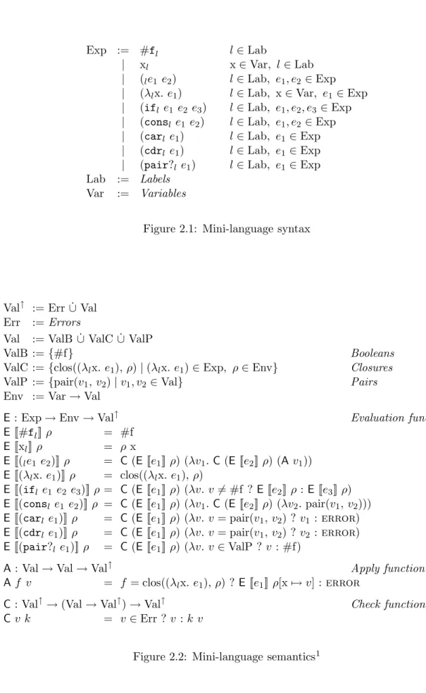
2.2 Language

Figure 2.1 presents the syntax of our small applicative functional language. It does not have a name but we will often refer to it as the mini-language. Expressions in the mini-language are labelled. The labels are used to give a unique “name” to the expressions. For example, it allows us to refer to a particular expression as e12 instead of having to write it verbatim

everywhere. We use numerical labels throughout this text.

The mini-language provides functions, pairs, and the Boolean ‘#f’. As in Scheme, anything except ‘#f’ is considered to be a true Boolean value when the ‘if’ expression tests its first sub-expression. The ‘pair?’ expression provides a way to distinguish between pairs and the other objects. Depending on whether its argument is a pair or not, it returns either the pair itself or ‘#f’, respectively. Finally, evaluation of sub-expressions generally proceeds from left to right. This particularity could make a difference if one of the sub-expressions loops and the other leads to an error, but it cannot when the program eventually terminates. The rest of the semantics of the language is fairly standard: the ‘if’ expression first evaluates the test and then only one of its two branches; the body of the λ-expression is evaluated only when the function is eventually called; the other expressions evaluate all of their sub-expressions.

Only three of the nine kinds of expressions require a dynamic safety test. We do not include pair?-expressions in these three as their purpose is not safety and there is no reason to expect their result to always be true (or false). Expressions accessing pairs, namely ‘car’ and ‘cdr’, must ensure that the objects that they are about to access are truly pairs. Calls must ensure that the objects returned by the evaluation of the first sub-expression are truly functions. The task of our type analysis is to give the optimiser the opportunity to remove as many safety checks as possible among those introduced by these expressions.

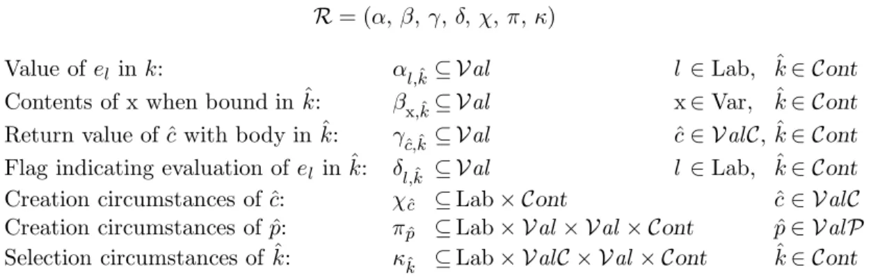
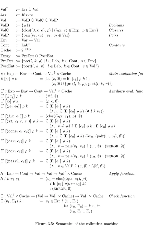
The detailed semantics of the language are presented in Figure 2.2.1 _{Semantic domain}

(30)

Exp := #f_l l ∈ Lab

| xl x ∈ Var, l ∈ Lab

| (le1 e2) l ∈ Lab, e1, e2 ∈ Exp

| (λlx. e1) l ∈ Lab, x ∈ Var, e1 ∈ Exp

| (ifl e1 e2 e3) l ∈ Lab, e1, e2, e3 ∈ Exp

| (consl e1 e2) l ∈ Lab, e1, e2 ∈ Exp

| (carl e1) l ∈ Lab, e1 ∈ Exp

| (cdrl e1) l ∈ Lab, e1 ∈ Exp

| (pair?l e1) l ∈ Lab, e1 ∈ Exp

Lab := Labels Var := Variables

Figure 2.1: Mini-language syntax

Val↑ := Err ˙∪ Val Err := Errors

Val := ValB ˙∪ ValC ˙∪ ValP

ValB := {#f} Booleans

ValC := {clos((λlx. e1), ρ) | (λlx. e1) ∈ Exp, ρ ∈ Env} Closures

ValP := {pair(v1, v2) | v1, v2 ∈ Val} Pairs

Env := Var → Val

E: Exp → Env → Val↑ Evaluation function

E[[#fl]] ρ = #f

E[[xl]] ρ = ρ x

E[[(le1 e2)]] ρ = C (E [[e1]] ρ) (λv1. C (E [[e2]] ρ) (A v1))

E[[(λlx. e1)]] ρ = clos((λlx. e1), ρ)

E[[(ifl e1 e2 e3)]] ρ = C (E [[e1]] ρ) (λv. v 6= #f ? E [[e2]] ρ : E [[e3]] ρ)

E[[(consl e1 e2)]] ρ = C (E [[e1]] ρ) (λv1. C (E [[e2]] ρ) (λv2. pair(v1, v2)))

E[[(carl e1)]] ρ = C (E [[e1]] ρ) (λv. v = pair(v1, v2) ? v1 : error)

E[[(cdrl e1)]] ρ = C (E [[e1]] ρ) (λv. v = pair(v1, v2) ? v2 : error)

E[[(pair?l e1)]] ρ = C (E [[e1]] ρ) (λv. v ∈ ValP ? v : #f)

A: Val → Val → Val↑ Apply function

Af v = f = clos((λlx. e1), ρ) ? E [[e1]] ρ[x 7→ v] : error

C : Val↑ → (Val → Val↑) → Val↑ Check function C v k = v ∈ Err ? v : k v

(31)

Val↑ contain evaluation results, which are either normal values or error values. We do not explicitly define the error values. Normal values (or simply, values) are the Boolean, from ValB, closures, from ValC, or pairs, from ValP. A closure is a constructor containing a λ-expression and the definition lexical environment. Note that pairs and environments can only contain values, not error values.

The evaluation function computes the value of an expression in a certain lexical environ-ment. It makes extensive use of the check function C to verify whether the values obtained during the evaluation of sub-expressions are normal. C takes an evaluation result and a continuation. It immediately returns the evaluation result if it is an error, otherwise it passes it to the continuation, which does the rest of the computation. The apply function A takes care of the details of the invocation of a closure on an argument. The specification of the evaluation function E itself is quite straightforward.

Note the situations in which an error can occur: in the access to the car- or cdr-field and in a call. Evaluation of the other expressions is always safe, barring the occurrence of an error in the evaluation of a sub-expression.

2.3 Generality of the Objective

Despite the fact that the objective of our research is done on type analysis, namely the removal of dynamic safety type tests, we expect the research to have a much broader impact. We present a few reasons to support our belief.

The mini-language is applicative; that is, the argument expression is completely evalu-ated before the closure is invoked with the result. However, that does not mean that the scope of our research is limited to applicative languages. We could aim at the same objective while using a lazy language. The task of type analysis would be similar in such a language.

The choice of a type analysis is a reasonable one, too, as performing a good type analysis in a dynamically-typed language is not less difficult than performing some other analysis. Instances of analyses include escape analyses [53], reference counting analyses [35], numerical range analyses [26, 27, 41, 48], and representation analyses [54, 32, 33]. In all cases, relatively simple analysis methods can lead to relatively good analysis results. However, doing an

(32)

optimal job, that is, obtaining results that allow the optimiser to do the best job possible, is uncomputable as all the desired properties depend on the actual computations done be the program.

Note that our real goal is not necessarily to obtain the best possible method to remove dynamic type tests in the code generated by compilers. We also want to study the efficiency of a demand-driven approach as a mean to drive an adaptive analysis intelligently. Non-adaptive methods clearly have intrinsic limitations that are more or less easily encountered. On the contrary, adaptive methods can push these limitations much farther. However, there has to be some mechanism to guide the adaptations. As will be presented in the following chapters, type analysis of the programs is performed using an adaptable analysis framework and a demand-driven approach provides the means to translate the needs of the optimiser (the task of removing safety tests) into precise directives on how to adapt the analysis of the program to obtain analysis results that are more useful to the optimiser. Although the demand-driven approach that we develop in this research is quite specific and the idea of being demand-driven is quite general, success in our particular project would bring evidence that the general idea can be useful.

The restriction to whole program compilation is not a mandatory one. In a concrete implementation, our type analysis could be adapted to support separate compilation while guaranteeing complete safety. However, a certain cooperation from the programmer would be required. First, the program would have to be separated in module. This way, no mutation of a variable could be done from another module (if the language includes side-effects). Second, the programmer would have to give type annotations for all variables that are exported out of a module. The importation of a module into a module under compilation would make these annotations available to the compiler. The more precise these annotations, the higher the quality of the analysis results for the module, and the higher the quality of the executable code. In order to ensure safety of the evaluation of the program, the compilation of each module would include a verification that the module conforms to the given annotations and, at run time, before the start of the normal evaluation of the program, the executable would perform a verification to ensure that each importing module has seen the same annotations than those truly declared in each imported module.

The restriction to a language without input/output is not mandatory either. We chose not to consider I/O because it does not add any interesting problem from the point of

(33)

view of the type analysis. It is clear that the ability to write data does not change what the programs compute and it would not interfere with the type analysis. So output is not interesting. It is less clear that the ability to read data is also uninteresting. Indeed, the data that are read have an impact on the computations that programs perform. They introduce an uncertainty factor in the computations. However, this uncertainty is quite easy to manage: a (read) expression may return any value that the language’s specification allows as a valid input value. For example, the specification could say that (read) returns a value made of pairs and Booleans every time it is evaluated. Consequently, any attempt by the type analysis to obtain precise type information about the possible value of (read) plainly fails.

Clearly, a type analysis is useful in the compilation of dynamically-typed languages. But it may seem useless for statically-typed languages such as ML or Haskell. However, it is not the case. The main reason is that these languages both provide algebraic types. An algebraic type may include many constructors. For example, in Haskell, list types are algebraic types including two constructors: ‘[ ]’ of arity 0 for the empty list and ‘:’ of arity 2 for the pairs. The programmer can define a function taking lists as an argument and use pattern-matching with a pattern for only one of the two constructors. If the function is passed a list built using the other constructor, an error occurs. For example, an error actually occurs if the head or the tail is extracted from an empty list. The inspection of the argument is a kind of safety dynamic test as the typing of the program cannot guarantee that only the expected constructor(s) will be passed. A type analysis such as ours would be required in order to remove as many of those tests as possible. If we reverse the point of view, programs in our mini-language can be considered to be statically typable using a unique type that includes three constructors. The uniqueness of this hypothetical type makes the static typing trivial and leaves all verifications relative to the constructors to the run time.

Object-oriented languages could also benefit from an adaptation of our type analysis. The exact instantiation class of an object can be seen as a constructor. The class of a de-clared variable can be seen as an algebraic type including all the constructors corresponding to its sub-classes. Moreover, the case where a variable does not reference any object, that is, when its value is null, can be seen as corresponding to an additional ‘null’ constructor.

(34)

we decided to use this particular applicative dynamically-typed functional mini-language because it is the kind of language that needs and stresses type analysis the most. First, programs written in dynamically-typed languages typically need more safety type tests than those in statically-typed languages. Second, functional programs have a tendency to have a more complex control-flow because of the use of higher-order functions. So our mini-language (which is similar to Scheme) is particularly challenging for a type analyser.

Finally, demand-driven analysis could be useful in the field of dynamic compilation, or just-in-time compilation. Of course, it would have to operate within relatively limited resources, especially in time. But the advantage is that analysis would operate while the program runs and profiling statistics about the real execution would be available.

(35)

Analysis Framework

This chapter presents the analysis framework and numerous properties related to it. The analysis framework, by itself, is not a complete static analysis for programs drawn from the syntactic domain Exp. An abstract model has to be provided to the framework in order to create an instance of analysis. Recall that the abstract model specifies what the phony values and phony evaluation contexts are when a phony execution of the program is performed. From now on, we designate phony values as abstract values and phony contexts as contours. The abstract model takes the form of a few framework parameters. This parameterisation of the analysis framework brings the mutability of the analysis that we need. Indeed, the framework has a great flexibility as will be made apparent by results in this chapter.

We start the presentation of the analysis framework by describing its external behaviour, that is, the description of its parameters and that of the results of an analysis instance. Next, we present the functioning of the framework. The rest presents different properties of the framework. The first one is the fact that any analysis instantiated from the framework always terminates. Next, a collecting machine is introduced. The machine computes the same result as the standard semantics for the mini-language but it also produces a cache containing the details of the computation. With the help of the collecting machine, we demonstrate that the analysis instances are conservative, that is, the results they produce represent at least all the concrete computations made during the concrete evaluation. Next, we show that for any program that terminates without error, there exists an abstract model showing that all dynamic type tests can safely be removed. We also show that, unfortunately, it is undecidable to determine if such a model actually exists for an arbitrary program. We

(36)

end the chapter by illustrating the flexibility of the framework by giving abstract models with which it is possible to imitate many known analyses.

A kind of analysis framework was previously presented by Ashley and Dybvig in [11]. It is parameterised by two modelling functions: one that controls the accuracy of the analysis by splitting abstract evaluation contexts and one that controls the speed of the analysis by performing widening on stores. In simple words, widening is some sort of “exaggeration” of the abstract values to help the analysis results to reach a stable state faster. Their analysis framework does not offer the subtlety that ours does. Both parameters have a global effect on the analysis. We consider them to be too coarse for our application. Also their framework handles mutable variables and data structures. This adds unnecessary complexity since our language is purely functional.

3.1 Instantiation of an Analysis

Before we present the process of instantiating an analysis for a program, we need to mention the existence of a few restrictions imposed on the program itself. Let el0 ∈ Exp be the

program to analyse. First, the framework requires the program to be α-converted. That is, each variable in the program must have a distinct name. This restriction poses no big problem since, for a program having variables with the same name, a simple renaming remedy to the situation. Second, the program must include proper labelling, that is, all labels have to be distinct. It is vital to uniquely identify each expression in the program in order to analyse it properly. Once again, there is no problem there since labels are an artificial creation, anyway. They are introduced for analysis purpose only. Third, the program has to be closed, that is, it must not have free variables. This restriction is closely related to our choice not to provide input/output operations in the mini-language (see Section 2.3).

Now, if we suppose we have an appropriate program el0, the analysis of el0 using an

abstract model M is denoted by

R = FW(el0, M)

where FW is the analysis framework receiving a program and a model, and returning analysis results R. We first describe the abstract model. Then the analysis results are presented.

(37)

M = (Val B, Val C, Val P, Cont, ˆk0, cc, pc, call)

Val B 6= ∅ Abstract Booleans

Val C 6= ∅ Abstract closures

Val P 6= ∅ Abstract pairs

Cont 6= ∅ Contours

ˆ

k0 ∈ Cont Main contour

cc : Lab × Cont → Val C Abstract closure creation pc : Lab × Val × Val × Cont → Val P Abstract pair creation call : Lab × Val C × Val × Cont → Cont Contour selection

where Val := Val B ˙∪ Val C ˙∪ Val P subject to |Val | + |Cont| < ∞

Figure 3.1: Instantiation parameters of the analysis framework

3.1.1 Framework Parameters

The abstract model, formed by framework parameters, is presented in Figure 3.1.1 The model includes abstract values, abstract contours, and abstract evaluation functions.

The abstract values include Booleans (Val B), closures (Val C), and pairs (Val P). Val B, Val C, and Val P are finite, non-empty sets. That is, these abstract domains must be finite in order to guarantee that the abstract evaluation of the program always uses a finite amount of resources. And they must be non-empty in order to have at least one abstract representative for the concrete values of each type. The three sets must be mutually disjoint, as it is expressed by the use of the disjoint union operator ( ˙∪). The set of abstract values Val is the union of the three sets. As soon as three sets conform to the mentioned constraints, they can be considered as legal abstract value domains. Nothing special is required of the abstract values themselves. Their type comes from the fact that they belong to one (and only one) of the three sets.

The abstract contours are given by the set Cont. It must be a finite, non-empty set. No other restriction applies to the abstract contours. Contours are abstract representatives for concrete evaluation contexts. A concrete evaluation context describes the circumstances in which an expression gets evaluated. It includes the current lexical environment that is visible by the expression. It also includes the identity of the caller to the closure which led

(38)

to the current evaluation, the caller of the caller, etc. The context usually has an impact on the value of an expression. For instance, an expression may produce different values when evaluated in different lexical environments during concrete interpretation. Similarly, this expression may produce different abstract values when evaluated in different contours during abstract interpretation.

Each abstract contour represents a certain fraction of all possible evaluation contexts. The abstract evaluation of an expression el in a contour ˆk must summarise everything

that could happen during the concrete evaluation of el in any evaluation context that is

represented by ˆk. For example, if el evaluates to a pair in a certain evaluation context and

to a closure in another context, and that both evaluation contexts are abstracted by ˆk, then, during abstract evaluation in contour ˆk, el will evaluate to at least an abstract pair and an

abstract closure, the last two being abstract counterparts of the concrete values returned by el.

Parameter ˆk0 is the contour in which the program (the top-level expression el0) is to be

abstractly evaluated. Except for that special use, ˆk0 is an ordinary contour.

When a λ-expression is abstractly evaluated, an abstract closure must be produced. Similarly for a cons-expression. However, the analysis framework does not decide by itself which closure or which pair should be returned. This is where the closure creation function (cc) and the pair creation function (pc) come into play. Function cc chooses the abstract closure from Val C that should be returned based on the λ-expression and the current con-tour. Function pc does the same but has also the possibility to base its decision on the two values that go into the abstract pair. We explain in the next sections what it means to produce a value that contains other values. pc may choose the abstract pair in function of the label of the cons-expression, or in function of the contour, or in function of the type of the value that goes in the cdr-field of the pair, or, in general, according to a combination of strategies. As long as cc returns an element of Val C and pc returns an element of Val P, everything works.

The possibility of specifying Val C and Val P contributes to the flexibility of the work but it is especially because of the existence of the cc and pc functions that the frame-work is very flexible. It is also because of the call function that we describe below.

(39)

func-tion). Indeed, Booleans are produced by the evaluation of the false constant and sometimes by pair?-expressions. There could have been a bc function. However, we do not see the utility of such a function as there is just one concrete Boolean. What would be the benefit of choosing one abstract Boolean over another one since they all represent the same con-crete Boolean? We believe there is none. But why do we allow Val B to have more than one element in the first place? In fact, there is no advantage, but there is no problem in doing so, either. The decision of having no bc function could be changed in the future if something indicates that it would be beneficial. The current treatment of Boolean creation by the framework is that each time an abstract Boolean is to be produced, the whole Val B set is returned.

The last framework parameter is the call function. This function selects contours in which expressions are evaluated. It is not used before the evaluation of each individual expression but only before the whole body of a closure. A (possibly) new contour is selected each time a closure is called. Indeed, when an abstract closure ˆc is invoked on argument ˆ

v in call expression (lel1 el2) and in contour ˆk, the body of ˆc gets evaluated in contour

call(l, ˆc, ˆv, ˆk). Hence, the call function contributes greatly to the flexibility of the analysis framework as different contours can be selected, depending, of course, on the invoked closure but also on the argument, on the label of the call expression where the invocation occurs, and on the contour in which this invocation occurs. The resulting flexibility allows our framework to have contours that may be call-chains or that may be abstract representatives of the lexical environment, etc. Examples of various uses of the call function can be found in Section 3.7.

In order to be a legal model for the analysis of a program el0, M has to obey to a last

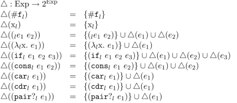
constraint. The three creation (or selection) functions have to be defined on the part of their from-set that covers at least every possible argument passed by the analysis framework. That is, their domain must cover at least every possible argument. The functions are not required to be defined on their whole from-set as the label argument poses a problem. Presumably, Lab is an infinite set and the rest of the specification of models manipulates only finite sets. So now we present the part of the from-set that must be covered by each function. Let us denote by 4(el0) the set of labels in program el0.2 Closure creation function cc has to be

defined at least on 4(el0) × Cont. Pair creation function pc has to be defined at least on

(40)

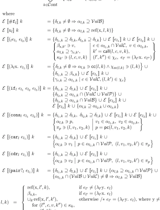
R = (α, β, γ, δ, χ, π, κ)

Value of el in k: α_l,ˆ_k⊆ Val l ∈ Lab, ˆk ∈ Cont

Contents of x when bound in ˆk: β_x,ˆ_k⊆ Val x ∈ Var, ˆk ∈ Cont Return value of ˆc with body in ˆk: γ_c,ˆ_ˆ_k ⊆ Val ˆc ∈ Val C, ˆk ∈ Cont Flag indicating evaluation of el in ˆk: δ_l,ˆ_k ⊆ Val l ∈ Lab, ˆk ∈ Cont

Creation circumstances of ˆc: χˆc ⊆ Lab × Cont ˆc ∈ Val C

Creation circumstances of ˆp: πpˆ ⊆ Lab × Val × Val × Cont p ∈ Val Pˆ

Selection circumstances of ˆk: κkˆ ⊆ Lab × Val C × Val × Cont ˆk ∈ Cont

Figure 3.2: Analysis results of the framework

4(e0) × Val × Val × Cont. And contour selection function call has to be defined at least on

4(e0) × Val C × Val × Cont.

We could relax this last constraint on the domain of the abstract creation functions a little more. For instance, the label passed to cc can only be that of a λ-expression. For pc and call, the label can only be that of a cons-expression and a call expression, respectively. However, specifying the minimal domains that way would be unnecessarily heavy. Anyway, the given specification does not pose a real problem as, for example, cc may return any element of Val C it wishes if the argument label is not one of a λ-expression; it does not matter.

3.1.2 Analysis Results

The analysis results R of the analysis of program el0 using model M are described in

Figure 3.2. R takes the form of seven matrices of abstract variables. Each matrix contains a certain kind of information. In fact, it is directly with these matrices that the framework does the analysis of programs.

We describe the contents of each matrix. Essentially, the first four matrices are the analysis results that are normally considered as the most interesting, especially the first. The last three are rather intended for internal purpose.

The α matrix indicates the set of values to which each expression evaluates to in each contour. Typically, there are many entries that remain empty after the analysis, because, for example, there is some dead code in the program or, by the way the model is built, some

(41)

expressions simply do not get evaluated in certain contours.

The β matrix indicates the values that each variable of el0, in each contour, may contain.

Note how the entries in this matrix require el0 to be α-converted. Identical names for

different variables would produce pollution in the results as the values of all variables sharing a certain name would also share their contents. The meaning of an abstract variable like β_x,ˆ_kis quite subtle. It is not necessarily equivalent to the result of a reference to x in contour ˆ

k. This would be ill-defined as there is no direct relation between the contour that prevails when x is (abstractly) bound to a value and the contour that prevails when x is referenced. The reference may occur inside of the body of a closure originating from a λ-expression that is in the scope of x. Remember that the contour possibly changes during each invocation. The abstract variable β_x,ˆ_k represents the value of variable x if x is the parameter of some closure ˆc and if, for every invocation where ˆc gets called on a certain value, contour ˆk is the one that is prescribed by call for the given situation. For example, consider the following program excerpt: . . . (1e2 e3) . . . (λ4x. (λ5y. x6)) . . .

Suppose that during evaluation of call e1 in contour ˆk, a closure ˆc, coming from λ-expression

e4, gets called on some value ˆv, and that call(1, ˆc, ˆv, ˆk) = ˆk0. Then, it follows that ˆv ∈ β_x,ˆ_k0.

Now, suppose that a closure originating from λ-expression e5 gets called and that its body

is evaluated in contour ˆk00. Then, the reference to x in e6 in contour ˆk00 will include the

contents of β_x,ˆ_k0 (and not of β_x,ˆ_k00) because ˆk0 is the contour in which x was bound.

The γ matrix indicates the values returned by the closures. Abstract variable γ_c,ˆ_ˆ_k contains the values returned by closure ˆc when its body has been evaluated in contour ˆk.

The δ matrix indicates in which contours each expression gets evaluated. Each entry of the matrix acts as a flag. If δ_l,ˆ_k is non-empty, then expression el gets evaluated in

contour ˆk, otherwise, it is not. The actual contents of these abstract variables are not important. The role of the δ matrix is to help the framework to generate analyses that are not too conservative. Analyses should always be conservative, but it should avoid