Characterization of heavy precipitation on Corsica

(1)

TH `

ESE

TH `

ESE

En vue de l’obtention du

DOCTORAT DE L’UNIVERSIT´

E DE

TOULOUSE

D´elivr´e par : l’Universit´e Toulouse 3 Paul Sabatier (UT3 Paul Sabatier)

Pr´esent´ee et soutenue le 25/11/2016 par :

Phillip SCHEFFKNECHT

Characterization of Heavy Precipitation on Corsica

JURY

Sylvain Coquillat LA, Toulouse President du Jury

Silvio Davolio _{ISAC-CNR, Bologna} _Rapporteur

Daniel Kirshbaum McGill University,

Montr´eal

Rapporteur

Chantal Claud LMD, Paris Examinatrice

V´eronique Ducrocq CNRM-GAME, Toulouse Invit´ee

´

Ecole doctorale et sp´ecialit´e :

SDU2E : Oc´ean, Atmosph`ere, Climat

Unit´e de Recherche :

Laboratoire d’A´erologie (UMR 5560)

Directeur(s) de Th`ese :

Dominique LAMBERT et Evelyne RICHARD

Rapporteurs :

(2)

(3)

(4)

(5)

Acknowledgements

First of all, I want to thank my supervisors Dr. Evelyne Richard and Dr. Dominique Lambert, who guided my work throughout this large endeavor. Thank you for the tips, the help and the guidance but also thank you for the funny moments we had during our meetings and for all the help during my early time in Toulouse. Special thanks to Evelyne for giving me my first home away from home in her house when I arrived in France. And thank you to Dominique for sending me on a trip to Corsica, so I could see the island about which I was writing for more than three years.

I would like to thank the members of my jury, starting with the president Prof. Sylvain Cocqillat. I thank Dr. Silvio Davolio and Prof. Daniel Kirshbaum for reviewing and evaluating my thesis. Their comments helped to further improve the manuscript for this final version. Thanks to the jury members Dr. Claude Chantal and Dr. Véronique Ducrocq as well as the members of my comité de thèse, Dr. Véronique Ducrocq and Dr. Andreas Wieser, who provided additional guidance.

Thanks to Prof. Daniel Kirshbaum for supervising my internship at McGill University in Montreal, which was a great experience. Special thanks to his wife, Rachel Shafts, without whom I might never have made it through the the bureau-cracy of the immigration process. Also, thank you to the anonymous Canadian customs officer at the Montreal airport who decided to give me my work permit on the spot instead of sending me back home, when I arrived in Canada before having received the offical work permit.

Thank you to Thibaut Dauhut for the countless discussions, great evenings and the visit in Montreal. I met him as a colleague but he became a good friend. Thank you to those who shared my office, Micha¨el Faivre, Allan Hally, and Daria Kuznetzova for the discussions, on and off-topic. Thanks to Thibaut Dauhut and

(6)

Jean-Fran¸cois Ribaud for helping me with buying and building all my furniture and thanks to David Baqu´e for helping me to move twice.

In addition, I want to thank the two Meso-NH wizards at the Laboratoire d’Aérologie, Juan Escobar and Didier Gazin, as well as Christine Lac, Gaëlle Delautier and Soline Bielli from Meso-NH support for patiently answering all my questions. Thank you to all Ph.D. students, post-docs, permanents and others with whom I shared a beautiful time at the Laboratoire d’Aérologie and in Toulouse and thank you all for the beautiful gifts I received on the day of my defense.

I thank my parents and my brother for supporting me through all my life and all my decisions, and last but most of all I want to thank my girlfriend, Karin. I left you to live abroad for 1251 days, yet you, Karin, kept supporting me. You are everything I could ever wish for!

(7)

R´

esum´

e de l’introduction en

fran¸cais

La pluie est essentielle pour la vie en général et les humains en particulier. Tout au long de l’histoire les centres de civilisation se sont implantés près des rivières, des fleuves, des lacs ou de la mer. Bien que la présence d’eau réponde à un besoin élémentaire, elle est en même temps un facteur de risque. Les précipitations intenses - et les inondations qui en découlent - causent régulièrement d’importants dégâts matériels, voire de nombreuses victimes. Il est donc important de bien comprendre les processus physiques impliqués dans ces évènements afin de mieux les prévoir et de permettre aux populations concernées de prendre les précautions nécessaires.

De telles pr´eoccupations sont au coeur du programme de recherche interna-tional HyMeX (Hydrological Cycle of the Mediterranean Experiment)1

dédié à l’étude du cycle hydrologique dans le bassin méditerranéen (Drobinski et al., 2014). En France, HyMeX constitue une des composantes du meta-programme MISTRALS2

(Mediterranean Integrated STudies at Regional And Local Scales). Durant l’automne 2012, la communauté HyMeX a organisé une vaste campagne de mesures spécifiquement consacrée aux précipitations intenses (Ducrocq et al.,

1

http://www.hymex.org

2

(14)

2014). Celle-ci a permis de documenter de nombreux évènements ayant affecté les côtes espagnoles, fran¸caises et italiennes

Les travaux menés dans cette thèse s’inscrivent dans le cadre général d’HyMeX. Ils sont focalisés sur les évènements précipitants intenses qui affectent la Corse. Ceux-ci possèdent en effet des spécificités qui leurs sont propres en raison du caractère à la fois montagneux et insulaire de la région impactée. L’approche utilisée repose sur la confrontation de simulations numériques conduites avec le modèle Méso-NH aux observations recueillies pendent la campagne HyMeX de l’automne 2012.

Contexte g´

eographique

Le bassin méditerranéen est situé entre l’Afrique au sud, l’Asie à l’est et l’Europe au nord. Ses côtes sont densément peuplées et donc vulnérables. Son climat est très contrasté avec des zones désertiques au sud et des zones tempérées au nord. Les contrastes pluviométriques sont particulièrement marqués entre les rives sud du bassin très arides et les côtes est de l’Adriatique où sont enreg-istrées des précipitations annuelles supérieures à 3000 mm qui en font une des régions les plus pluvieuses d’Europe. Une autre caractéristique majeure du basin méditerranéen réside dans la présence de nombreux reliefs côtiers qui induisent un système de vents locaux complexe. Les zones côtières exposées au flux marins sont fréquemment frappées par des fortes pluies qui sont principalement observées en automne dans l’ouest du basin et davantage en hiver dans sa partie orientale (see, e.g., Froidurot et al., 2016; Jansa et al., 2000, 2001; Morel and Sénési, 2002a,b; Ri-card et al., 2012; Rysman et al., 2016; Trigo et al., 2002). Dans la perspective d’une augmentation de la fréquence de ces évènements intenses (Blanchet et al., 2016;

(15)

Homar et al., 2010; Gao et al., 2006), de gros efforts sont pour mieux comprendre les m´ecanismes impliqu´es et la fa¸con dont ils interagissent.

Située dans le bassin nord occidentale, la Corse (Fig. 1.2) est une ˆıle montag-neuse qui culmine à 2706m au Monte Cinto et dont près de 120 sommets dépassent les 2000 m. La chaˆıne de montagne centrale, globalement orientée nord sud, con-stitue un obstacle au vent zonal. Durant la campagne HyMeX, différents sites instrumentés ont été déployés en Corse. La Corse possède en effet le double intérêt d’être une zone cible (susceptible d’être impactée par de fortes précipitations) et une zone amont (permettant d’observer les précurseurs des systèmes précipitants qui vont impacter les côtes du sud-est de la France et de l’ouest de l’Italie). Par ailleurs, du fait de son caractère insulaire, la Corse constitue un laboratoire na-turel pour observer les interactions entre des flux marins peu perturbés et une orographie complexe.

Les m´

ecanismes physiques

Les précipitations intenses sont associées au phénomène de convection profonde qui conduit à des systèmes nuageux à fort développement vertical. Ce phénomène nécessite trois ingrédients majeurs: une colonne atmosphérique conditionnellement instable, une fort apport d’humidité ainsi qu’un mécanisme de soulèvement. Ce dernier peut avoir des causes multiples telles que le soulévement orogrographique ou la présence de zones de convergence d’origine thermique ou dynamique qui peuvent agir isolément mais aussi se combiner. Les nombreux travaux réalisés jusqu’alors illustrent parfaitement la complexité des interactions possibles entre convection et orographie ainsi que les nombreux défis qu’elles posent aux modèles de prévision du temps.

(16)

Objectifs du travail et plan de la th`

ese

L’objectif central est d’améliorer la connaissance des processus physiques impliqués dans les évènements de fortes pluies en Corse et de mieux comprendre leur in-teraction avec la topographie complexe de l’ˆıle. Afin de mieux caractériser ces évènements nous nous intéressons tout d’abord à leur climatologie. L’étude porte sur 31 ans d’observations pluviométriques et de réanalyses météorologiques. Les méthodes utilisées reposent sur une analyse en composantes principales et un al-gorithme de classification. Le travail se poursuit par l’étude détaillée des trois épisodes qui ont affecté la Corse durant l’automne 2012. Le premier (4 septembre 2012) est associé à une profonde dépression quasi-stationnaire. Il a généré de très fortes précipitations principalement le long de la côte est de l’ile. Le second cas d’étude (31 octobre 2012) se caractérise par une dépression qui s’est rapidement déplacée depuis les ˆıles Baléares vers le nord de la Corse. Enfin Le cas du 23 Octobre 2012 correspond à un épisode de convection profonde quasi-stationnaire qui s’est développée sur une ligne de convergence située en mer au sud-ouest de la Corse. Chaque cas est discuté dans le contexte de la climatologie puis simulé avec le modèle Méso-NH. L’approche est systématique et consisiste à réaliser des en-sembles de simulations initialisées à partir de différents jeux de conditions initiales et de couplage aux frontières latérales. En outre, la sensibilité à la résolution hor-izontale du modèle est étudiée en comparant les résultats obtenus aux résolutions de 2.5 et 0.5 km. Différents tests de sensibilité pour lesquels la topographie du modèle a été modifiée complètent l’étude.

(17)

Chapter 1 General Introduction

Rain is an essential factor for human civilization. Cities have always been built where access to fresh water was available and over the course of history long term shifts in precipitation patterns have caused the dawn and downfall of entire empires. However, over shorter time spans precipitation can also vary greatly de-pending on the location. Droughts can eradicate harvests and cause famines and shortage of fresh water for humans, animals and plants alike. On the other end of the spectrum, heavy precipitation events (HPEs) are capable of devastating areas of up to thousands of square kilometers, endangering the lives of countless people and causing enormous economic damage. HPEs can cause landslides, flooding, erosion, and damage to buildings and infrastructure, e.g. roads, train lines, elec-tricity grids, and freshwater supply. Thus a deep understanding of precipitation and the involved mechanisms is of the utmost importance for any populated area around the world.

As part of the HyMeX (Hydrological Cycle of the Mediterranean Experiment)1 program, this work aims to provide a better understanding of the mechanisms of heavy precipitation on the Mediterranean island of Corsica. The primary tools

1

(18)

1.1. GEOGRAPHICAL CONTEXT - THE MEDITERRANEAN BASIN

are numerical simulations of the events and the comparison to observations gath-ered during the respective events. This chapter represents a general introduction by presenting the geographical context of the studies, the HyMeX program and a short history of numerical weather prediction. The atmospheric scales are ex-plained and their implications for the challenges in current weather models are presented shortly. In addition, the basic physical processes of convective insta-bility and the mechanisms of heavy precipitation are presented, with a focus on orographic precipitation and the interaction of convection with underlying terrain. This is followed by a selection of literature on HPEs focusing on the Mediterranean basin and in particular on Corsica. Lastly, the goals and outline of this work are presented, concluding the general introduction.

1.1 Geographical Context - The Mediterranean

Basin

For thousands of years, the Mediterranean sea (see Fig. 1.1) has been one of the centers of civilization and it has a densely populated coast with complex orography and a diverse climate. The Mediterranean sea is located between Europe in the north, Asia in the east, Africa in the south, and the Atlantic ocean in the west, to which it is connected through the strait of Gibraltar. It lies between the temperate regions of western and central Europe in the north and the Sahara desert in the south. In fact, the Mediterranean climate is extremely diverse, ranging from arid conditions in north Africa (see, e.g., Thornes et al., 1998) to one of the wettest regions of Europe along the mountain ranges east of the Adriatic (see, e.g. Mehta and Yang, 2008). During the summer, the weather is relatively dry with regular heat waves (more than once per year on average between 1950 and 1995, Thornes et al., 1998).

(19)

1.1. GEOGRAPHICAL CONTEXT

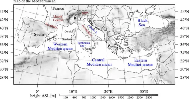
Figure 1.1: Map of the Mediterranean with geographical references and terrain height contours.

The Mediterranean is split into three main basins. The western Mediterranean is located between the Iberic peninsula, France, Italy and north Africa, the central Mediterranean is located south of Italy and southwest of Greece and the eastern Mediterranean is located between Greece, Turkey, Egypt and Libya. In the north-east the Mediterranean is connected to the Black sea via the Bosporus, which separates Europe and Asia. A smaller side arm, the Adriatic, extends north be-tween Italy and Croatia, Montenegro, Albania, and Greece.

In addition to the diverse climate, the orography around the Mediterranean, and also on some of its larger islands, is highly complex. Several mountain ranges border the sea, the most important ones around the north of the western Mediter-ranean basin being the Apennines in Italy, the Alps in central Europe, the Massif Central in southern France, and the Pyrenees at the border between Spain and France. These mountain ranges impact the air flow into the western Mediterranean

(20)

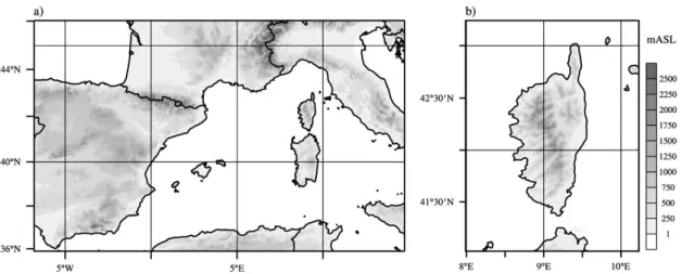
1.1. GEOGRAPHICAL CONTEXT

Figure 1.2: Map of Corsica with geographical references and terrain height con-tours.

basin and, depending on the wind direction, can directly impact the upstream con-ditions of HPEs.

Corsica (Fig. 1.2) is located in the north of the western Mediterranean, between Italy in the north and east, Sardinia in the South, and continental France in the northwest. Corsica has a north-south extent of about 180 km and an east-west extent of about 80 km. A mountain range covers the island in north-south direction. Its highest peak, Monte Cinto, is 2706 m high and around 120 other summits are higher than 2000 m.

The coasts and islands of the Mediterranean basin are often struck by dev-astating high precipitation events (HPEs), which occur predominantly in autumn (winter) over the western (eastern) Mediterranean (see, e.g., Froidurot et al., 2016; Jansa et al., 2000, 2001; Morel and S´en´esi, 2002a,b; Ricard et al., 2012; Rysman

(21)

1.2. THE HYMEX PROGRAM et al., 2016; Trigo et al., 2002). In the prospect of a probable increase of such HPEs (Blanchet et al., 2016; Homar et al., 2010; Gao et al., 2006), a considerable amount of effort is made to better understand the involved mechanisms.

1.2 The HyMeX Program

The HyMeX program (Ducrocq et al., 2014) is an international program aimed at a better understanding of the hydrological cycle of the Mediterranean sea. It is part of the MISTRALS2

(Mediterranean Integrated STudies at Regional And Local Scales) program. One central aspect of HyMeX is the exploration of the mecha-nisms behind HPEs. In addition, the impact of climate change on the Mediter-ranean is explored, since this region is one of the hot-spots of climate change, facing both, an increase in HPEs and droughts. In the framework of the program, a database3

was set up to host a large amount of operational and program-specific observations as well as the output of multiple numerical models.

Part of the HyMeX program is a large field campaign in the Mediterranean. The long observation period (LOP) takes place from 2010 until 2020, spanning about 10 years, and its goal is to gather long-term hydrological, oceanographic, and meteorological observation throughout the entire Mediterranean basin. An enhanced observation period (EOP) took place from mid 2011 to mid 2015, with an emphasis on research observations. During autumn 2012 and spring 2013, two special observation periods (SOPs) took place. Their focus lay in the northwestern Mediterranean, particularly the Spanish and French coasts, Italy, the Balearic Islands, Corsica, and Sardinia. SOP 1 (5 September to 6 November 2012) was dedicated to the observation and modeling of HPEs and SOP 2 (1 February to 15 March 2013) was dedicated to the observation of strong winds and their impact

2

http://www.mistrals-home.org

3

http://mistrals.sedoo.fr/HyMeX/

(22)

1.2. THE HYMEX PROGRAM

on the ocean mixed layer, dense water formation and ocean convection. The SOPs are divided into multiple intense observation periods (IOPs), which are associated with the individual events observed during each SOP. An IOP is thus limited to the region where the HPE occurred. In addition, IOPs can be split into multiple parts if the same system moved over multiple regions, e.g. IOPs 15a, b, and c, which took place over Catalonia, the C´evennes, and Corsica from 20 to 23 October 2012.

During SOP 1, instruments were deployed all along the northwestern coast of the Mediterranean. On Corsica, the Karlsruher Institut f¨ur Technologie (KIT) deployed a number of instruments. Their KIT-Cube, a collection of instruments dedicated to the exploration of the turbulence, moisture, and aerosols of the bound-ary layer, was located in Corte, in the north of Corsica (see Fig. 1.2). In addition, the KIT provided multiple atmospheric soundings a day during several IOPs. The balloons were launched in San Giuliano at the east coast, where an X-band re-search radar was also deployed by the KIT (Fig. 1.2), among other instruments. These instruments complement the operational network on Corsica, which consists of roughly 125 surface station, an operational weather radar in Al´eria and the op-erational radiosoundings from Ajaccio (at 00 and 12 UTZ, see red markers in Fig. 1.2).

The atmospheric observatory CORSiCA4

(Corsican Observatory for Research and Studies on Climate and Atmosphere-ocean environment, Lambert et al., 2011) was set up on Corsica, serving both HyMeX and the Chemistry-Aerosol Mediter-ranean Experiment (ChArMeX). Lastly, the SAETTA (Suivi de l’Activit´e Elec-trique Tridimensionnelle Totale de l’Atmosph`ere) has been deployed on Corsica since 2014 in the framework of CORSiCA . All these programs are aimed toward

4

(23)

1.3. NUMERICAL WEATHER PREDICTION a better understanding of the Atmosphere and the Ocean in the Mediterranean, continuing an effort that has been going on for centuries.

1.3 Numerical Weather Prediction

This thesis relies heavily on the usage of numerical simulations of high precipitation events. With regard to this focus, a short history of numerical weather prediction as well as current challenges are presented in this section. While the increasing availability of computational resources greatly increased the potential for the usage of numerical models, it also comes with new challenges, which are explained below.

1.3.1 The Beginning of Numerical Weather Prediction

Even though the first attempts at weather prediction were made more than 2000 years ago, the bulk of the knowledge about precipitation and its prediction has been acquired during the last century. Specifically, the succession of low and high pressure which accompanies the changing weather in the mid latitudes was only understood as recently as around 100 years ago. The atmosphere is a large dynamic system and its accurate description requires the knowledge of its state, which is only obtained by observations at multiple locations over a large area. These have to be sufficiently dense in space and time (see, e.g., Bjerknes, 1919). Because of this, meteorology was one of the first disciplines which made wide use of the early means of telecommunication.

Vilhelm Bjerknes (1916) was the first to explain cyclones as resulting from disturbances in the westerly winds, which are often found in the mid-latitudes. His work was then validated by his son, who developed an empirical model of a mid-latitude cyclone based on surface observations (Bjerknes, 1919) and described rain as result of lifting processes along fronts and orographic barriers (Bjerknes

(24)

1.3. NUMERICAL WEATHER PREDICTION

and Solberg, 1921). They also explained mid latitude cyclones as resulting from disturbances in the polar front and provided the first schematic model of the mid-latitude circulation (Bjerknes and Solberg, 1922).

The idea and attempt of numerical weather prediction predate the advent of the first computers by more than two decades. Undergoing the process of discretizing the thermal and dynamical fields of the atmosphere and their governing equations in space and time requires a large number of calculations, making it impossible to do even in real time without the help of computers. The first attempt, however, was done by Richardson (1922). He attempted a 6-hour forecast of the surface pressure using a set of discretized equations. It took Richardson 6 weeks to calculate just two vertical columns and he estimated that for a horizontal grid size of 200 km

”64000 computers [referring to persons doing the calculations manually, author’s note] would be needed to race the weather for the whole globe” (Richardson, 1922,

p. 219). Unfortunately, his forecast for the change in surface pressure was wrong by two orders of magnitude due to an imbalance of wind and pressure in his initial conditions. Removing these imbalances would take another 20 years.

The upper level structure of the mid-latitude atmosphere was described by Rossby et al. (1939), who developed the theory of what we nowadays know as barotropic Rossby-waves. This theory was refined by accounting for the earth’s curvature (Haurwitz, 1940) and extended to a baroclinic atmosphere (Bjerknes and Holmboe, 1944). Based on their work, Charney (1947) presented a way to re-move acoustic waves and shearing-gravitational oscillations from the perturbation equations, eliminating the problems that prevented the success of Richardson in 1922. These equations formed the basis of later work (Charney, 1949; Charney and Eliassen, 1949), which led to the first successful computer-based numerical weather forecast (Charney et al., 1950), obtained by numerical integration of the barotropic vorticity equation. Over the following decades, computational power

(25)

1.3. NUMERICAL WEATHER PREDICTION has grown exponentially, allowing smaller grid spacings and time steps, the use of more complete sets of equations and more sophisticated parametrizations for subgrid processes such as microphysics and turbulence. However, this progress has its challenges.

1.3.2 Atmospheric Scales - Synoptic, Meso- and

Micro-scale

Weather models are based on the equations that govern the evolution of a given state (pressure, temperature, moisture, wind) of the atmosphere over time. Values of the fields are discretized onto a number of points which are distributed on a grid that covers either the entire globe or a limited region. Typically, the values at a certain grid point are then viewed as representative for the entire grid cell. A basic property of the computational grid is the distance between its points which equates to the grid cell size.

For global models, the grid spacing is often in the tens of kilometers while for localized weather models in research applications the horizontal grid spacing can reach less than 100 m. Atmospheric phenomena also have typical scales. Rossby waves span over thousands of kilometers and the surface low and high pressure systems can become equally large. On the other end of the scale, turbulent eddies are found everywhere in the atmosphere with sizes down to the fraction of a mil-limeter. Between the synoptic (large) and the microscale a range of phenomena can be found in the mesoscale (Orlanski, 1975), like frontal circulations, convec-tive systems, orographically induced circulations or sea and land breeze systems. Depending on the phenomenon, a grid spacing of few kilometers down to around 100 m is necessary to capture the relevant processes. As a result, certain mesoscale phenomena are sometimes represented by a limited number of grid points or they might fall entirely within just one grid cell.

(26)

1.3. NUMERICAL WEATHER PREDICTION

In order to fully capture all relevant motions of turbulent flow in a simulation, one would have to resolve all scales of motion. The minimum size of turbulent eddies which have to be resolved does have a lower limit (Kolmogorov, 1941), but unfortunately it is beyond any reasonable grid spacing currently achievable in weather models. The scale of these eddies, the Kolmogorov-microscale, depends on the kinematic viscosity ν and is given by

η = ν 3 ǫ !14 , (1.1) where ǫ = u3

/l, and u and l are the velocity and length scale of the energy

con-taining eddies (Bryan et al., 2003; Kolmogorov, 1941). The turbulent eddies which would need to be resolved in deep moist convection are of the size of approximately 3 · 10−4 _{m, requiring grid spacings of around 0.1 mm (Bryan et al., 2003), which} would allow the direct numerical simulation (DNS) of turbulent flow. A 50 by 50 by 20 km domain for the simulation of an isolated convective cell would have 5 · 1016

- in words: ten quadrillion - grid points.

To circumvent these extreme resolution requirements, turbulent processes are parametrized. There are two main approaches, the first one being large eddy simu-lations (LES), which depend on the explicit representation of an inertial subrange (energy containing scale). This is generally not accomplished with grid spac-ings much larger than 100 m. The second approach is to parametrize processes which are not represented at grid spacings of several kilometers and more. Such parametrizations primarily handle planetary boundary layer processes like vertical mixing, turbulence and heat flux. Between 100 m and several kilometers is a gap, for which no appropriate turbulence parametrizations exist (Bryan et al., 2003; Wyngaard, 2004). Within this range, processes included in the parametrization schemes begin to be explicitly represented in the simulations. Nevertheless,

(27)

mod-1.4. THE PHYSICS OF HEAVY PRECIPITATION EVENTS els are regularly used at grid spacings within this gray zone (Wyngaard, 2004) and despite the shortcomings in model design they produce valuable results.

1.4 The Physics of Heavy Precipitation Events

Deep moist convection (DMC) is involved in a large number of Mediterranean HPEs (see, e.g. Davolio et al., 2009; Doswell et al., 1998; Ferretti et al., 2000; Jansa et al., 2000, 2001; Lambert and Argence, 2008; S´en´esi et al., 1996; Tapiador et al., 2012; Trapero et al., 2013). For deep moist convection to occur, three ingredients are required: conditional instability, low level moisture, and lift (Doswell et al., 1996; Doswell, 1987).

1.4.1 Convective Instability

In this work, instability refers to the stability of the atmosphere with respect to the vertical displacement of an air parcel. This section gives a short overview of convective instability in the atmosphere (for a comprehensive explanation, see, e.g. Holton, 2004, p. 289–298). Due to the vertical pressure gradient in the atmosphere a dry vertically displaced air parcel cools down as it ascends. The cooling rate is given by the dry adiabatic lapse rate

−dT_dz = g

cp

= Γd, (1.2)

where g = 9.81 m s−2 _{is the the gravitational acceleration and c}

p = 1005 J kg−1 is the heat capacity of air at constant pressure. In the lower atmosphere Γd is approximately constant at 9.76 K km−1_{. If the vertical temperature lapse rate} −dT/dz is larger than Γd, i.e. the atmosphere is statically unstable, any upward (downward) displaced parcel will become positively (negatively) buoyant and

(28)

1.4. THE PHYSICS OF HPES

tinue to ascend (descend). However, if the atmosphere is statically stable any upward (downward) displacement will cause the parcel to become negatively (pos-itively) buoyant and buoyancy will act as a restoring force, pushing the parcel back to its original level. This restoring force can lead to buoyancy oscillations in the atmosphere. The frequency of these oscillations is given by

N2 = gd ln θ dz = g θ dθ dz, (1.3) where N2

is called the Brunt Väisälä frequency, θ is the potential temperature, and z is the altitude. In summary, static stability in a dry atmosphere depends on the vertical temperature gradient

−dT_dz                  > Γd, N2 < 0 statically unstable = Γd, N2 = 0 statically neutral < Γd, N2 > 0 statically stable (1.4)

With the addition of moisture, latent heat has to be considered. If a moist parcel is lifted, it will cool until its temperature is equal to its dew point, at which point the water vapor will begin to condense. The level at which this happens is called lifting condensation level (LCL). The condensation of water vapor converts latent energy into sensible heat, thereby slowing down the cooling of the parcel as it ascends. The lapse rate at which the parcel cools is called the pseudoadiabatic lapse rate Γs = − dT dz = Γd 1 + Lc/(RT ) 1 + ǫL2 cqs/(cpRT2) (1.5) where ǫ=0.622, qs is the saturation mixing ratio, R is the gas constant for dry air, and Lc ≈ 2.5 · 105 J kg−1 is the latent heat of condensation. In the lower atmosphere, Γs is approximately 6 to 7 K km−1. For a lapse rate Γs < Γ < Γd

(29)

Figure 1.3: Simple example of the vertical profile of a conditionally unstable atmo-sphere. Temperature T (dew point Td) of the environment are shown by the black (blue) lines. The black and blue dashed lines show T and Td for the dry adiabatic ascent of a parcel from the surface, the pink line shows the moist adiabatic ascent above the LCL.

the atmosphere is stable to vertical displacement of unsaturated air parcels but unstable to the vertical displacement of saturated parcels. Saturation is a necessary condition for this instability, which is therefore called conditional instability. We call θ∗

e the equivalent potential temperature of a hypothetically saturated parcel. The use of θ∗

e is to underline the necessary condition (saturation), because while

θe is well defined for unsaturated parcels, the statements on stability do not apply without saturation being present. For Γs it follows that dθe∗/dz = 0.

(30)

1.4. THE PHYSICS OF HPES dθ∗ e dz                  < 0 conditionally unstable = 0 saturated neutral > 0 conditionally stable (1.6)

From its origin, a lifted parcel undergoes dry adiabatic ascent (dashed black in Fig. 1.3) as long as it is unsaturated. As it reaches its LCL, the freed latent energy slows down the cooling and it continues its moist adiabatic ascent (conserving θe, pink in Fig. 1.3). During the first part of its ascent, the parcel is cooler than its environment and negatively buoyant. The energy necessary to overcome this phase is called convective inhibition (CIN), and it has to be provided by external forces. Above the level of free convection (LFC), the temperature of the parcel is higher than that of the environment, allowing it to rise on its own. The parcel continues to accelerate until it reaches the equilibrium level (EL), sometimes also referred to as level of neutral buoyancy (LNB). Convective clouds often show an overshooting top where rising air moves past its EL before slowing down and descending again. Integrating buoyancy force along the parcel’s path between the LFC and the EL yields the convective available potential energy (CAPE). CAPE and CIN are given by CAP E = Z zEL zLF C gTparcel− Tenv Tparcel and CIN = Z zLF C z0 gTparcel− Tenv Tparcel (1.7)

By this definition, CAPE is positive and CIN is negative. However, both are usually given in absolute values. In the simplified skew-T diagram (Fig. 1.3), CIN (CAPE) is represented by the cyan (yellow) area. For deep moist convection to occur, initial lift is necessary to overcome convective inhibition and reach the LFC. This initial lift can come from orographic lifting or lifting above a convergence zone. Diurnal heating can also heat the boundary layer and gradually erode CIN

(31)

1.4. THE PHYSICS OF HPES until deep convection is initiated. Often a combination of such processes will act. Assuming a perfect energy conversion, the upper limit imposed on the vertical velocity by CAPE is

wmax = √

2CAP E. (1.8)

In practice, entrainment (mixing of cool dry air into the convective plume) and friction will prevent any rising parcel from reaching wmax. The initiation of deep moist convection is difficult to predict because the initial lifting can happen due to small scale processes which are not resolved in numerical models.

1.4.2 Orography and its Effect on Air Flow and

Precipita-tion

Since the Mediterranean is surrounded by multiple high mountain ranges and some islands have mountains in excess of 2000 m, orographic effects play an essential role in Mediterranean HPEs. The interaction between orography and air flow has been repeatedly studied for decades, but even idealized mountain shapes and constantly stratified layers of dry air introduce a number of different phenomena. In the simple 2D case (an infinitely long ridge) and homogeneous cross-mountain flow the effect is limited to relatively simple topographic waves. Variation of the cross-mountain wind or the stability with height allows the formation of lee waves which can extend hundreds of kilometers downstream of mountains (Durran, 1990). When air flow encounters a mountain, one primary question is whether the flow will traverse the obstacle or be blocked by it. The parameter that helps to determine the answer is the Froude number

F r2 = u¯ 2 c2 = ¯ u2 gLc , (1.9)

where ¯u is the mean environmental wind speed, c2

is the shallow water wave speed (see, e.g. Holton, 2004, p. 287), and Lc is the characteristic length. The Froude

(32)

number F r can be understood as the ratio of kinetic and potential energy. For

F r < 1 (subcritical) flow will tend to be blocked by an obstacle while for F r > 1

(supercritical) the flow will pass over the obstacle. For F r ≈ 1 the linear solution breaks down. The flow is subcritical upstream of the obstacle, turns supercritical above the obstacle and tends to form a downslope windstorm in the lee with a hydraulic-jump-like feature, where the flow adjusts back from super- to subcritical in a turbulent zone (Durran, 1990). In real case scenarios, the applicability of these concepts is somewhat limited, as the atmosphere is neither homogeneously stratified nor is the flow horizontally or vertically homogeneous. Reinecke and Durran (2008) presented a way to estimate the resulting flow regime for real cases. They use the mountain height normalized by a scale for the vertical wavelength of a linear 2D hydrostatic mountain wave, sometimes also called inverse Froude number (see also Smith, 1989a)

ˆh = N h

u , (1.10)

where N is the Brunt Väisälä frequency, h is the mountain height and u is the cross mountain wind speed. One method to determine ˆh proposed by Reinecke and Durran (2008) is to measure u and N below the mountain height and then take the average over the layer below h to calculate ˆh.

Even in dry homogeneous flow, simple setups can produce complex solutions, such as stagnation points (Smith, 1989b), lee vortices, wakes (Schär and Smith, 1993a) and vortex streets (Schär and Smith, 1993b). The above mentioned phe-nomena are also observed in the atmosphere, such as the wake of Madeira (Grubiˇsić et al., 2015), and they can also be relevant for regional weather phenomena, like the cyclogenesis supported by Alpine blocking (Egger, 1988; Pichler et al., 1990), which also occurs over the Gulf of Genoa (Trigo et al., 2002).

Taking moisture into account introduces a number of additional mechanisms, which happen primarily due to the conversion between latent and sensible heat. If

(33)

1.4. THE PHYSICS OF HPES the lifting is sufficient to produce clouds, latent heat is converted into sensible heat, changing the stability profile. If rain forms, it will fall out of the cloud into the unsaturated layer below and start evaporating, thereby cooling the air beneath the cloud and forming a cold pool. Even over an idealized 2D mountain a simple setup such as a moist nearly neutral flow with constant u can lead to complex effects, such as downslope windstorms, convective cells and upstream mid-level drying (Miglietta and Rotunno, 2005). In conditionally unstable flow, rain was found upstream and downstream of the 2D mountain for weak and intermediate u (2.5 and 10 m s−1_{) and over the mountain for strong u (20 m s}−1_{). Convection initiated} along the windward slope produced a cold pool which propagated upstream when

u was weak (Miglietta and Rotunno, 2009). The highest rainfall amount was

seen for simulations where u balanced the upstream propagation of the cold pool, resulting in quasi-stationary convection which allowed large accumulations of rain (Miglietta and Rotunno, 2009, 2010). It was also found that a sheared profile with cross mountain wind in the boundary layer and weaker or no cross mountain wind aloft allows the formation of deeper and more intense convective cells (Miglietta and Rotunno, 2014). Real cases are vastly more complex because the terrain, airflow and moisture are inhomogeneous 3D fields which change over time.

A comprehensive review of orographic effects on rain is available in Houze (2012). Figure 1.4 shows schematic illustrations of orographic mechanisms. Moist air which encounters orography and follows its slope upward forms an orographic cloud when stable (Fig. 1.4a) or convective cells when unstable (Fig. 1.4b). In addition, the terrain itself may induce diurnal wind systems which in turn can lead to the formation of clouds. During the day, heating causes warm upslope flows (Fig. 1.4c) and during the night, radiative cooling along the surface induces downslope flows, which can lead to convergence along the base of the mountain (Fig. 1.4d). A mountain may also locally directly enhance precipitation by orographic lifting (Fig.

(34)

(35)

1.4. THE PHYSICS OF HPES 1.4e) or increase precipitation originating from a higher non-orographic cloud, the ”seeder” (Fig. 1.4f), where the lower cloud is referred to as ”feeder”. Topographic waves may trigger convective cells downstream of the mountain (Fig. 1.4g) or locally enhance preexisting convection (Fig. 1.4h). A cold pool forming beneath a precipitating cloud can be fully (Fig. 1.4i) or partially (Fig. 1.4j) blocked and act as an obstacle which provides lift. Figure 1.4k shows a mechanism by which dry flow over a mountain can result in a capping inversion, which allows conditional instability to build up. Figure 1.4l shows one possible way to release this built up instability by overcoming convective inhibition via warm upslope flow over a hill. Considering the wide range of mechanisms which can work together to influence the formation of clouds, convective cells and precipitation, it is not surprising that the detailed explanation of such events can be difficult. The precise forecasting of orographic precipitation also poses a challenge, especially if it occurs in connection with DMC (see, e.g. Hanley et al., 2011).

1.4.3 Heavy Precipitation Events in the Mediterranean

Ricard et al. (2012) showed that long-lasting HPEs over southern continental France and Corsica are mostly associated with quasi-stationary trough-ridge pat-terns, high CAPE values over the western Mediterranean and a moist troposphere. Low level jets (LLJ) advect moisture from the sea toward the coast, where the HPEs occur. These unstable inflows together with lifting above orography or along convergence lines lead to DMC, which can either occur alone or embedded into larger, stratiform precipitation systems.

Duffourg and Ducrocq (2011) analyzed recent events over southern France in an attempt to explore the origin of the moisture supply. They found that the main sources of moisture for the studied HPEs were evaporation over the Mediter-ranean and advection from the Atlantic. Ducrocq et al. (2008) looked at three

(36)

HPEs over southern France and analyzed the mesoscale ingredients for stationary events. They identified orographic lift and lifting along the edge of cold pools as primary lifting mechanisms. In all cases, a conditionally unstable LLJ was imping-ing on an obstacle, supplyimping-ing the convective system with moisture and an inflow of potentially unstable air.

Numerical models can help tremendously in understanding single events as well as the involved processes. Before the wide availability of mesoscale models, Ducrocq et al. (2002) found that models with a grid spacing of 2.5 km are well capable of outperforming low resolution (10 km) models. However, this improve-ment required that the initial conditions were well captured. They even found that poorly captured initial conditions could reverse the results, causing the high resolution simulations to perform worse than the low resolution simulations. Since then, the availability of computational resources has increased drastically and grid spacings of 2.5 km and less have become feasible even for operational purposes. Nevertheless, small changes in initial conditions can cause large differences on the mesoscale, especially when convection is involved. Thus, large efforts have been made to explore and improve the capability of such high resolution models. Hally et al. (2014a,b) explored the potential of a stochastic ensemble by adding random perturbations to model physics. They analyzed their results in terms of disper-sion of the precipitation forecast and found that this approach has the potential to assess the sensitivity of HPEs. However, they also found the initial conditions to be the most important criterion. Fresnay et al. (2012) used the same method, including tests with a grid spacing of 500 m. They found that at this higher res-olution the ensemble shows a larger sensitivity to perturbations in model physics. Instead of perturbing only one microphysical scheme, Tapiador et al. (2012) cre-ated an ensemble by using different schemes not only for microphysics but also for cumulus parametrization and the land surface. In addition, they tested perturbed

(37)

1.4. THE PHYSICS OF HPES initial conditions. Their results show that using multiple schemes resulted in a larger spread than the perturbed initial conditions.

Numerous case studies using numerical models have been conducted to learn more about the details of HPEs in the Mediterranean region. Doswell et al. (1998) showed that heavy precipitation in the Mediterranean region can be associated with different processes, such as DMC but also orographic enhancement of precip-itation below a relatively stable air mass. S´en´esi et al. (1996) studied the Vaison-La-Romaine flash-flood event in southern France. They found that a cut-off low and its slowly moving cold front led to a squall line. The slow movement of the system led to large precipitation accumulations. Trapero et al. (2013) studied a catastrophic 1982 flash-flood event in the Pyrenees, which affected Spain, Andorra, and France. They found a quasi-stationary extratropical cyclone advecting moist air toward the Pyrenees. Buzzi et al. (1998) studied a HPE over the Piedmont in northwestern Italy in 1994. They determined the local orography as an im-portant factor, which influences precipitation by forcing orographic lifting. Buzzi et al. (1998) also conducted sensitivity tests by deleting parts of the orography and changing model physics. They found that removing the terrain caused the HPE to shift downstream while changes in evaporative cooling and latent heating controlled the formation of cold pools and the capability of the air to move over orography, respectively. Ferretti et al. (2000) confirmed the importance of orogra-phy and orographic lifting for that particular event. It was later found that the 1994 Piedmont flash flood was intensified by dryer air from the east which was blocked by the Alps and deflected westward, increasing convergence beneath the convective cells (Rotunno and Ferretti, 2001). Davolio et al. (2009) studied a HPE which occurred at the Adriatic coast. It was caused by convergence of a northeast-erly barrier jet along the Alps and a southeastnortheast-erly moist LLJ from the Adriatic sea. In a comprehensive analysis of multiple events, Davolio et al. (2016) found

(38)

that the precipitation distribution over northeastern Italy depended heavily on the thermodynamic profile of the incoming flow. Flow over the Alps tends to produce heavy precipitation over the orography whereas blocked flow leads to the forma-tion of a barrier jet and upstream convergence, displacing the precipitaforma-tion and convection over the flat terrain of the Po valley. Further east, similar events can occur. Kotroni et al. (1999) studied a HPE which occurred in 1997 over Greece. They also found DMC as a result of orographic lifting ahead of the cold front to be responsible.

All these events were associated with a cyclone and all of them were charac-terized by DMC. The interaction between orography and moist LLJs also plays a crucial role in the above mentioned cases. These ingredients common for HPEs along the coast of the Mediterranean and over its islands, however, they are not exclusive to the Mediterranean. Lin et al. (2001) found that very moist low level jets, conditionally unstable flow impinging on orography, steep mountains, and quasi-stationary synoptic systems are ingredients common to HPEs worldwide. One example in a different region would be the Madison County flash flood of 1995, which was analyzed by Pontrelli et al. (1999) and which was also caused by the simultaneous occurrence of a moist LLJ, orographic forcing, and synoptic forcing due to a short wave trough. The processes mentioned above show how complex such events can be. In many cases the involved mechanisms stretch over multiple orders of magnitude starting from synoptic systems with hundreds up to thousands of kilometers in size via regional topography and air mass variations to the paths of individual embedded convective cells and updrafts measuring only hundreds of meters to a few kilometers. The task of unraveling the interactions between scales and processes is challenging.

(39)

1.4.4 Heavy Precipitation Events over Corsica

From a composite analysis of 8 HPEs over Corsica, Ricard et al. (2012) showed that moisture and CAPE were generally high between Sardinia and continental Italy. According to their findings, the main source of moisture lies to the south of the island with southerly flow in the boundary layer being the dominant direc-tion during HPEs over Corsica. The island and its interacdirec-tion with precipitating systems were the subject of several studies during the recent years. Lambert and Argence (2008) did a preliminary study of the HPE of 14 September 2006. They demonstrated one of the difficulties with current mesoscale case studies, namely that the verification of the simulation output is difficult. While obtaining clearly different results with two different input data sets, no conclusion was reached as to which simulation was better than the other. They also encountered problems when trying to reproduce the fine scale features of the event even though the large scale was well captured in both their experiments.

A more in-depth analysis was performed by Barthlott and Kirshbaum (2013), who analyzed isolated convection which occurred on 26 August 2009. The event was characterized by DMC over Corsica and Sardinia. They simulated the case using different stretching factors for the terrain height between 0 and 1.3 and also without islands. Their modeling experiments indicate that the mountains influenced the formation of convection via their diurnal circulation. However, even the temperature gradients between a flat island and the sea would have been sufficient for initiation of DMC due to convergence along the sea-breeze front. Only the complete removal of the islands from the simulation completely suppressed deep convection. This shows that different factors contribute to the formation of convection, including but not limited to sea-breeze, land-breeze and orographic circulations.

(40)

The role of Sardinia in DMC over Corsica was investigated by Ehmele et al. (2015), who looked at six events and conducted tests with standard orography as well as flat and deleted Sardinia. They found a decrease in precipitation for cases with strong synoptic forcing and no systematic change for cases with weak synoptic forcing. The role of Sardinia consists of blocking or deviating the large scale flow and modification of convection over Corsica via cold pools generated by convection over Sardinia.

An idealized study was conducted by Metzger et al. (2014), who placed Corsica as an isolated island in homogeneous flow. They used vertical profiles to initial-ize their simulations and varied the wind direction in 15◦_{steps. The tests were} conducted using constant winds of 2 and 5 m s−1_{. They also tested the effect of} increased instability and a reduced saturation deficit between 900 and 400 hPa. For the cases where DMC was simulated, it occurred on the lee side of the island, initi-ated by convergence. Metzger et al. (2014) found that lower wind speeds are more reliable in initiating DMC. For the higher (5 m s−1_{) wind speed they found that} northerly and southerly winds are capable of producing convection while easterly and westerly winds were not. Their conditions were highly idealized. Nevertheless, their findings show that convection can form in the lee of Corsican orography.

For the study of HPEs, the island of Corsica, forms a natural observatory in the northwestern Mediterranean Sea. It lies off the coast of northwestern Italy and on many occasions the upstream conditions for precipitation events in Liguria and Tuscany and even southern continental France can be measured on Corsica. On the island, a mountain range stretches from the north to the south with altitudes of over 2700 m above sea level (ASL). This makes Corsica the ideal place to study the influence of mountains on previously relatively undisturbed inflow into precipitating systems and their interaction with orography.

(41)

1.5. GOALS AND OUTLINE OF THIS THESIS

1.5 Goals and Outline of this Thesis

This work aims to contribute a better understanding of the processes which lead to the formation of HPEs over Corsica. To provide context, a climatology of HPEs is presented in Chapter 2, which is obtained by applying well established methods within the geographical context of Corsica and the Mediterranean, in order to produce a highly specialized climatology and classification of events. In addition, we present three heavy precipitation events which occurred during SOP1 of the HyMeX program in autumn of 2012. Each of these events represents a different class of event. The case of 4 September 2012 (Chapter 4) was caused by a quasi-stationary cyclone east of Corsica. The case of 31 October 2012 (Chapter 5) was caused by a fast moving cyclone which approached the island from the west. The case of 23 October (Chapter 6) was caused by localized quasi-stationary DMC which formed along a convergence line over the southeast of Corsica. Each case is discussed within the context of the climatology and their analysis yields examples for mechanisms which contribute to HPEs over Corsica. To account for the uncertainties in model design at the mesoscale, each case is tested for its sensitivity to model resolution by comparing simulations at 2.5 km and 500 m horizontal grid spacing. Lastly, Chapter 7 contains a summary of the results and an outlook on future research based on the findings in this thesis.

(42)

(43)

Chapter 2 Climatology of Rainfall on

Corsica

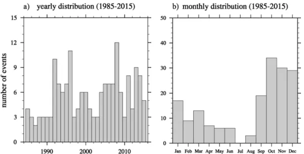
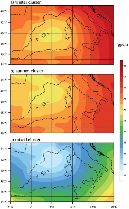
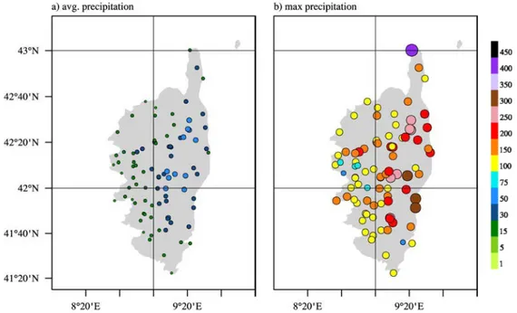
This chapter presents a 31 year (1985–2015) climatology of HPEs (>100 mm within 24 h) over Corsica. It seeks to answer the questions of how common such events are on Corsica and to analyze their seasonal cycle. In addition, a principal component analysis (Hannachi et al., 2007; Wilks, 2011) is performed on the ECMWF analysis data over the western Mediterranean to classify the HPEs. Three classes of events are identified and described. The methods used in this section are well established in atmospheric science. Here, they are applied to the western Mediterranean in an attempt to classify HPE over Corsica according to their geopotential and equivalent potential temperature θe fields and spatial distribution of precipitation. Section 2.1 contains a brief description of the climate in the Mediterranean and on Corsica, with focus on precipitation. The method used in this chapter is briefly explained in Section 2.2. Section 2.3 presents the seasonal distribution and mean fields, the EOFs and clusters are presented in sections 2.4 and 2.5, respectively. The physical interpretation of the clusters follows in section 2.6. The results are discussed in Section 2.7 and the conclusions are presented in Section 2.8.

(44)

2.1. THE CLIMATE OF THE MEDITERRANEAN

2.1 Current Knowledge on the Climate of the

Mediterranean

Precipitation in the Mediterranean follows a seasonal cycle. The summers are gen-erally dry and during the late summer precipitation increases in the west, where cyclogenesis is most often found over the Iberian peninsula (Trigo et al., 2002). During September, October and December, the heaviest precipitation moves grad-ually east (see, e.g. Kelley et al., 2012; Mehta and Yang, 2008; Trigo et al., 2002). For Corsica, the maximum is found from September to December. The region around Corsica also has an exceptionally high cyclone track density (Alpert et al., 1990; Nissen et al., 2010) with the Gulf of Genoa just north of the island being the most active cyclogenesis region from November to February (Trigo et al., 2002).

Mehta and Yang (2008) obtained a precipitation climatology for the Mediter-ranean basin based on 10 years (1998 - 2007) of TRMM measurements. They found that the highest precipitation is found over the mountainous regions of Europe, namely the Pyrenees, the Alps, the Apennines and the mountain ranges east of the Adriatic, in Slovenia, Croatia, Bosnia and Herzegovina, Montenegro and Albania. In these mountains, the average precipitation is between 2 and 4 mm d−1_{. On the} other end of the scale, north Africa receives only around 0.1 mm d−1_{. However,} the precipitation over the Mediterranean basin shows a seasonal cycle in intensity and location. Mehta and Yang (2008) found that the strongest precipitation oc-curs from September to March, with the peak months being October to January. While the peak month for the western Mediterranean (5-10◦_{E) is in November, the} peak occurs later further east (November and December at 10◦_{E and December to} January at 30◦_{E). In meridional direction, precipitation is located further north} in the Summer (values of >2 mm d−1 _{north of 45}◦_{N), the strongest precipitation} moves south until it peaks around 37◦_{N in November and December.}

(45)

2.1. THE CLIMATE OF THE MEDITERRANEAN Even though this cycle is well known, there are still considerable difficulties in its accurate representation. Kelley et al. (2012) simulated the weather over the Mediterranean from 1950 to 2000 using the Coupled Model Intercomparison Project phase 5 (CMIP5) and evaluated its results using observations. In their simulation, they found the typical seasonal cycle of higher precipitation in win-ter and lower precipitation in summer. However, their model showed a drying throughout the seasons with the strongest trend seen in March, April and May. The observations, on the other hand, show drying predominantly during winter. Gao et al. (2006) attempted to estimate the change in precipitation toward the end of this century by simulating the 1961-1990 and 2071-2100 periods using the IPCC A2 (highest) emission scenario. They found an increase of precipitation over the northern Mediterranean, primarily from December to January, mostly over the French coast, around Genoa and the northern Adriatic. They also found a moderate increase for the September to November period mostly over the west-ern Mediterranean. Their results also indicate an increase in extreme precipitation events over the northern Mediterranean.

A composite analysis for HPEs in the Mediterranean was done by Ricard et al. (2012). They examined the monthly distribution of HPEs (>150 mm day−1_{) from} 1967 to 2006 and found that the majority of events (70%) occur from August to De-cember with 20% in October alone. In addition, Ricard et al. (2012) examined the mesoscale environment of HPEs in four regions around the western Mediterranean (Languedoc-Roussillon, C´evennes-Vivarais, South Alps, and Corsica) based on a five year (2002-2006) climatology. For this period, they found a similar monthly distribution of events. They focused on the autumn period (August to December), and their analysis includes 40 HPEs observed from 2002 to 2006, 8 of which were located over Corsica.

(46)

2.1. THE CLIMATE OF THE MEDITERRANEAN

Their composite analysis identified a trough over the British islands and Spain with southwesterly flow aloft as an important ingredient to HPEs in the western Mediterranean. They found a moist LLJ over the western Mediterranean im-pinging on the orography along the northern coast and conditionally unstable air upstream of the HPEs. For Corsica, their composite analysis revealed that the highest moisture and instability is usually found southeast of the island, over the Tyrrhenian sea between Corsica, Sardina, Italy and Sicily. A trough is located over eastern Spain and a surface low is found centered north of the Balearic islands. The moist LLJ is found primarily east of Sardinia and Corsica, advecting warm and moist air from the Tyrrhenian sea toward the Corsican orography.

Cyclones are the primary cause of HPEs and their distribution over the Mediter-ranean has been repeatedly explored (see, e.g. Alpert et al., 1990; Campins et al., 2011; Maheras et al., 2001; Nissen et al., 2010; Trigo et al., 2002). Cyclone track-ing algorithms tend to also identify relatively weak thermal lows, increastrack-ing the number of detected cyclones substantially. Most of these thermal lows are weak, short lived, and stationary. Their occurrence shows a well detectable diurnal cycle (Campins et al., 2011). This is especially true for the summer, when such lows form predominantly over the Sahara and the Iberian peninsula (Alpert et al., 1990; Campins et al., 2011; Trigo et al., 2002). In winter, cyclogenesis happens predomi-nantly due to synoptic disturbances interacting with the baroclinicity found along the northern coast between the cold land and the relatively warm sea (Trigo et al., 2002). The Gulf of Genoa is the most active cyclogenesis region in the western Mediterranean, especially during winter (Alpert et al., 1990; Nissen et al., 2010; Trigo et al., 2002). The cyclones forming in the Gulf of Genoa show little to no diurnal cycle, deepen faster and are more intense than those of other cyclo-genesis regions (Maheras et al., 2001), and are often associated with lee cyclones

(47)

2.2. METHODOLOGY caused by Alpine blocking (Trigo et al., 2002). In the eastern Mediterranean most cyclogenesis occurs over Cyprus (Alpert et al., 1990).

2.2 Methodology

2.2.1 EOFs and Principal Components

In a meteorological context, fields such as temperature, pressure, moisture, etc. are often given as discrete points in time and space. Longer sequences of measurements at multiple locations can be given as a matrix with time along one direction and space along the other. In linear algebra, there are ways to decompose matrices in order to simplify them. One of these ways is based on the set of vectors which are made up by the lines of a matrix. This set of n vectors with m components, if linearly independent, are the basis of a vector space. It is possible to obtain a different basis for the same vector space which consists of all orthogonal pairwise different vectors. In addition, the basis can be defined such that the original matrix can be as closely as possible represented by a linear combination of as few basis vectors as possible. The method of obtaining such a basis is the calculation of equivalent orthogonal functions (EOFs) and principal components (PCs).

This section shall not go into detail on how the calculation is done, but the curious reader can find a short but detailed summary of the usage of EOFs in meteorology in Hannachi et al. (2007) (for a more comprehensive explanation, see, e.g., Wilks, 2011). The main goal of the calculation of EOFs and PCs is to reduce the dimensionality of the problem. In meteorology, most data sets have a large number of data points and this method can help to identify underlying patterns which can be described using a largely reduced number of dimensions. When reconstructing the original fields, the contribution of additional EOFs change the outcome gradually less, allowing in many cases a sufficiently accurate description

(48)

2.2. METHODOLOGY

of the full fields using a relatively (to the number of measurements) limited number of EOFs instead of the full data set.

In this section, multiple variables are used to account for multiple aspects of HPEs. The EOFs are calculated based on the 500 and 950 hPa geopotential and 950 hPa θe fields over the western Mediterranean. The atmospheric conditions are taken from ERA Interim (ECMWF re-analysis) data. For each of the fields the temporally averaged field for the corresponding date is used (00, 06, 12, and 18 UTC). Since the fields of geopotential and θe differ in their magnitude and variability, they are normalized before using them to calculate the EOFs. This is accomplished by subtracting the temporal mean and then dividing the data at each location by the standard deviation of the respective time series. The built in function of the NCAR1

Command Language (NCL)2

is then used to calculate the EOFs and PCs.

2.2.2 The k-means algorithm

The first two principal components form a two-dimensional vector for each event, equivalent to a point cloud in IR2. A clustering algorithm can then be used to find groups of points within this cloud. The algorithm chosen for the current climatology is the k-means algorithm (Hartigan and Wong, 1979), which is an iterative algorithm based on the distance between the points (see, e.g., MacQueen, 1967). The number of clusters has to be chosen beforehand (3 in this work). Before the first iteration, each of the n clusters is assigned a random centroid ck. In the

1

National Center for Atmospheric Research

2

(49)

2.2. METHODOLOGY first iteration, each point is assigned to the cluster of the closest centroid. After that, each iteration recalculates the position of each centroid such that

cn+1= 1 K K X k=0 xk, (2.1)

where cn is the centroid of the cluster at iteration n and xk are the k members of the cluster. At each iteration the centroid is set to the mean of the cluster. After this operation, the distance of each point xk to each centroid is checked and each point is assigned to the cluster whose centroid is closest to it. This process is repeated until no points change clusters. The energy of cluster n, En, is given by

En= K X k=1 (xk− ck) 2 (2.2)

and the total energy is

Etot = N

X

n=1

En, (2.3)

where N is the total number of clusters. Each time the algorithm finds a con-figuration where no point changes clusters, the cluster concon-figuration represents a local minimum of the function Etot(c1, c2, ..., ck). However, it is not necessarily the absolute minimum of the function. In fact, different initial configurations of the randomized centroids often lead to different configurations of the clusters with different values of Etot. Usually, the aim is to obtain a robust configuration of clusters. One way to do this, is to repeatedly run the algorithm with different initial values (given by random seeds) and analyze the results with respect to their

Etot and the number of occurrences of each configuration. Both can be used as an objective measure of the robustness of the clustering. For this particular case,

k-means was used with 100 different random seeds, all of which produced identical

clusters.

Characterization of heavy precipitation on Corsica

TH `

ESE

TH `

ESE

DOCTORAT DE L’UNIVERSIT´

E DE

TOULOUSE

Phillip SCHEFFKNECHT

Characterization of Heavy Precipitation on Corsica

Contents

R´

esum´

e de l’introduction en

fran¸cais

Contexte g´

eographique

Les m´

ecanismes physiques

Objectifs du travail et plan de la th`

ese

Chapter 1

General Introduction

1.1

Geographical Context - The Mediterranean

Basin

1.2

The HyMeX Program

1.3

Numerical Weather Prediction

1.3.1

The Beginning of Numerical Weather Prediction

1.3.2

Atmospheric Scales - Synoptic, Meso- and

Micro-scale

1.4

The Physics of Heavy Precipitation Events

1.4.1

Convective Instability

1.4.2

Orography and its Effect on Air Flow and

Precipita-tion

1.4.3

Heavy Precipitation Events in the Mediterranean

1.4.4

Heavy Precipitation Events over Corsica

1.5

Goals and Outline of this Thesis

Chapter 2

Climatology of Rainfall on

Corsica

2.1

Current Knowledge on the Climate of the

Mediterranean

2.2

Methodology

2.2.1

EOFs and Principal Components

2.2.2

The k-means algorithm