Would climate policy improve the European energy security?
Abstract
Energy security improvement is often presented as a possible co-benefit of climate policies. This paper evaluates this claim. It presents a methodology to investigate whether climate policy would improve energy security, while accounting for the difficulties entailed by the many-faceted nature of the energy security concept and the large uncertainties on the determinants of future changes in energy systems. To do so, it uses a set of indicators in a four-dimension analysis grid of the energy security concept, and a database of scenarios exploring the uncertainty space. The results, focusing on Europe, reveal there is no unequivocal effect of climate policy on all the dimensions of energy security and that some trade-offs are involved. The many-faceted nature of energy security matters: energy security has several dimensions, some of which can be heightened by climate policy. Time matters: the effect of climate policy on energy security depends on the time horizon considered. Last, these results are robust to key uncertainties on the future potential and costs of technologies, on future improvements in energy efficiency, on fossil fuel resources and markets and on drivers of economic growth. However, some of these uncertainties determine the magnitude of the effect of climate policy on energy security indicators.
Keywords: Climate policy, energy security, Europe, scenarios database, multi-criteria decision.
1. Introduction
Energy security and climate policy are strange bedfellows. Energy security concerns were one of the main motivations of the 1990 G7 held in Houston, the United States energy capital, and hosted by George H. Bush, with the aim of putting a “Climate Convention” on the international agenda (Kirton, 2007). At that time, there was hope that climate change could be used to convince the American public to accept the discipline needed to reduce oil dependence (Schlesinger, 1989). As a trick of history, energy security has undergone a recent revival of interest, triggered by high oil prices but also linked to the difficulties in
establishing an international climate architecture. The hope now is that some support for climate policies could be won by invoking their co-benefits in terms of energy security.
In one way or the other, energy security and climate policy are thus frequently presented as two aspects of the same issue. In a speech in the United States on October 20, 2006, Tony Blair declared that “we must treat energy security and climate security as two sides of the same coin” — which has since become a repeated refrain. The European Union (EU) is particularly involved in such an approach: both the Climate and Energy Package and the Energy Roadmap 2050 (European Union, 2011) endorse the goals of reducing greenhouse gas emissions while ensuring the security of energy supplies.
Are climate policy and energy security actually two sides of the same coin? They undeniably share a common root cause: increasing global demand for energy. But the solutions for improving energy security and reducing greenhouse gases are not necessarily the same, and may involve synergies or trade-offs. For example, energy efficiency and renewable technologies have been recognized as options to promote the two goals simultaneously (European Commission, 2001). Conversely, limiting coal use to reduce CO2 emissions could have negative impacts on the energy security of the many countries that have abundant coal reserves. Similarly, restricting the extraction of emission-intensive unconventional oil would increase the world’s dependence on oil from the Middle East (Hartley, 2008). It is therefore not clear whether climate policies would improve energy security or not, and this issue deserves closer scrutiny. This paper proposes a methodology to investigate the issue and applies it to the case in Europe.
We first review the small but growing literature that examines the links between climate policies and energy security (Section 2.1). This literature provides evidence for both synergies and trade-offs between climate policies and energy security. The difference in the results reported in these studies appears to be primarily due to different indicators chosen to measure energy security. This difficulty calls for an examination of the definition of energy security and of indicators to measure this concept, which we do in Section 2.2. We then build on the literature that explores the concept of energy security to propose four dimensions of this many-faceted concept, and to develop a set of indicators to measure the four dimensions.
A second difficulty arises when studying the effect of climate policy on energy security due to pervasive uncertainties on the determinants of future changes in energy systems — for instance population and economic growth, costs and the potential of technologies such as electric vehicles, renewable energies or synthetic fuels and consumer behavior with respect to energy services. This difficulty calls for an investigation of the uncertainty space to test the robustness or sensitivity of the results. In Section 3 we describe a methodology to build a large database of scenarios exploring the uncertainty space using an energy-economy-environment model, Imaclim-R, to account for this second difficulty.
In Section 4, we use the set of indicators we developed to analyze the database of scenarios, focusing on Europe. We find that, depending on the indicator used, conclusions concerning the effect of climate security on energy security diverge. Moreover, the time horizon matters: climate policy can have a negative effect on an indicator in the short term and improve it later. Lastly, the determinants of future changes in energy systems do not influence the set of indicators analyzed in the same way. Some indicators are robust to changes in assumptions on availability of low carbon technologies, for instance, while others are very sensitive.
2. Context
2.1.Evidence for both synergies and trade-offs
There is a small but growing literature that examines the issue of the links between climate policies and energy security. Evidence is provided for both synergies and trade-offs. Concerning synergies, Grubb et al. (2006) show that low-carbon objectives are associated with greater long-term diversity in electricity generation in the UK. McCollum et al. (2011) and McCollum et al. (2012) also show that concerted decarbonization efforts can increase the diversity of the energy supply, as measured by a compound diversity indicator aggregated at the global level. Rozenberg et al. (2010) show that climate policies reduce world vulnerability to oil scarcity, measured as the difference between the discounted Gross World Product in two scenarios with more or less oil resources. Consequently, climate policies appear as a hedging strategy against the uncertainty on oil resources, in addition to their main aim of avoiding dangerous climate change. Similarly, Maisonnave et al. (2012) conclude that unilateral EU climate policy provides protection against rising oil prices, as measured by lower GDP losses inferred by an exogenous scenario of oil prices rise in the case when climate policies are implemented than in the absence of climate policy. On the trade-offs side, Kuik (2003) shows a trade-off between economic efficiency of climate policies and energy security for the EU.
Other studies highlight synergies in some cases and trade-offs in others. For instance, Turton and Barreto (2006) conclude that stringent climate policies offer synergies with respect to the security of the oil supply (measured by the ratio of the resource to consumption), but trade-offs with respect to the security of the gas supply. IEA (2007) choses two indicators for energy security: a measure of the market concentration in each international fossil fuel market, weighted by the country’s exposure to each fuel (ESIprice), and the country’s share of total energy demand met by oil-indexed, pipe-based gas imports (ESIvolume). IEA’s analysis shows that different measures aimed at reducing CO2 emissions can have either positive or negative impacts on the two indicators. For instance, improvements in end-use efficiency have positive impacts on both indicators, while switching to biofuels for transport improves the ESIprice indicator but worsens the ESIvolume indicator. Brown and Huntington (2008) acknowledge that complementarity between a reduction in CO2 emissions and an improvement in energy security exist at the level of individual technologies, but that trade-offs arise when a mix of technologies is being selected to pursue both goals. The authors show that optimal policy could be adopting a suite of technologies that provide each benefit in only one dimension rather than relying on a few costly technologies that increase both energy security and reduce greenhouse gas emissions. In stringent climate change mitigation scenarios, van Vliet et al. (2012) show that the diversity of the primary energy supply mix increases in the emerging regions of Asia, while the effect on the imported share of total primary energy supply depends on the region: it increases in Centrally Planned Asia, mainly China, and decreases in South Asia, dominated by India.
This brief literature review highlights one difficulty in answering the question of the impact of climate policy on energy security due to the lack of clarity and a common definition of energy security concept and of indicators needed to measure it. Indeed, the different results in the aforementioned studies seem to be primarily due to different
indicators chosen by the authors. This difficulty calls for an examination of the definition of energy security and of indicators to measure this concept.
2.2.Selection of indicators to measure energy security
Although energy security is high on the policy agenda and pervasive in the discourse, it is seldom accompanied by a clear definition of the concept or a discussion of how to measure it.
A broad definition of energy security can be given by the negative, i.e. by defining its opposite: energy insecurity. Energy insecurity is the risk of the impact on welfare of either the physical unavailability of energy, or prices that are unaffordable or overly volatile (IEA, 2007). Energy security is about limiting this risk. Cherp et al. (2012) (Box 5.1) built an inventory of alternative definitions of energy security. Alternative definitions are also provided and analyzed by Winzer (2012), who concludes that, even though different definitions focus on various subsets of the threats to the energy supply chain, energy security is concerned with risk. Short-term energy security considers the risks of disruption of the energy supply due to strikes, extreme climate events, accidents, political unrest, etc.; while long-term energy security considers risks due to the depletion of fossil fuels and the unequal distribution of resources in the world. In this article, we focus on long-term energy security.
Translating this broad definition into operational ways to measure energy security is a difficult endeavor. But without clear measures, the analysis of the concept is bound to be vague and blurry. Three recent contributions (Kruyt et al., 2009; Chester, 2010; Sovacool and Brown, 2010) significantly advanced this endeavor. All three emphasize the many-faceted nature of the energy security concept, and all three propose a 4-dimensional grid of analysis. Two axes are common to the three contributions: the availability axis and the affordability axis. The availability axis groups elements related to the physical or geological existence of energy. The affordability axis includes the elements of costs for energy consumers.
The other two dimensions differ in the three studies, but can all be grouped under dependency, which measures the economy’s dependence on energy, and under sustainability, which accounts for the environmental impacts and societal acceptability of energy extraction and transformation technologies.
Table 1: Axes of the energy security concept and a selection of corresponding indicators to measure them
Axes of the energy security concept Selection of indicators
Availability Production/Resource (oil)
Concentration of markets (oil)
Dependence Energy intensity of GDP
Share of imports in TPES
Affordability Energy import bill/GDP
Households' energy budget
Sustainability Carbon content of TPES
Based on this approach, we select a set of indicators covering all the dimensions. We extend the availability dimension to include the concept of diversity. This concept can concern the whole range of suppliers of one type of energy - the more suppliers there are, the more resources will still be available if tensions appear concerning one of them -, but also the range of energy types on which a sector, or the whole economy, relies. For this dimension, we focus on oil because, among the three main fossil fuels (oil, gas and coal), it is both the most traded and the one with the lowest global resource: production ratio (Cherp et al. (2012), Table 5.6). We use the ratio of production to resources to measure its physical availability worldwide1. We add a diversity component to this dimension, measured by the concentration of oil markets. We use the Herfindahl-Hirschmann index, calculated as the sum of squared market shares of oil producers. Note that this index increases when the market is dominated by a small number of producers. These two indicators are global and not specific to Europe2.
For the dependence dimension, the energy intensity of GDP (the ratio of total primary energy supply, TPES, over GDP) measures the dependence of the economy on energy, and the share of imports in TPES measures the dependence of the energy supply on imports.
For the affordability dimension, instead of the absolute prices of energy types that do not account for the fact that some energy types might become expensive over time but also less used, we focus on the energy import bill as a share of GDP and on the share of households’ budget devoted to energy.
We chose two indicators for the sustainability dimension: the carbon content of TPES and the installed nuclear capacity, a technology that involves problems of acceptability.
Table 1 summarizes the indicators used in this paper to evaluate the different dimensions of energy security. The indicators are calculated such that an increase (respectively decrease) in their value indicates a worsening (respectively improvement) in the dimension of energy security they measure. This selection of indicators is necessarily based on a number of arbitrary choices, and other indicators could also be appropriate. Nevertheless, they are representative of the indicators frequently discussed in the literature, although not generally examined all together. Finally, the selection presented here results in a trade-off proposing (i) a limited number of indicators to ensure the results are readable, (ii) a variety of indicators covering the four axes of the energy security concept, (iii) indicators that can be calculated with the model used in this article.
3. Method
3.1.The Imaclim-R model
Imaclim-R is a hybrid simulation model of the world economy (Sassi et al., 2010; Waisman et al., 2012) that presents changes in the macro-economic and technological world in a consistent framework. It is disaggregated into 12 regions and 12 sectors, including five
1 It is more common to present the inverse ratio, i.e. resources over production, expressed in years of reserves
remaining at the current rate of extraction. However, we present the ratio of production to resources, so that the value of the indicator increases when the availability dimension worsens.
2
energy sectors: coal, oil, gas, refined products and electricity. Europe is one of the 12 regions. Details on the regional and sectoral disaggregation can be found in Appendix B. The model is calibrated on the 2001 base year by modifying the input-output tables provided by the GTAP-6 dataset (Dimaranan and McDougall, 2006) to make them fully compatible with 2001 IEA energy balances (in Mtoe) and data on passengers’ mobility (in passenger-km) from Schafer and Victor (2000). The model covers the period 2001-2100 in yearly steps through the recursive succession of static equilibria and dynamic modules.
The static equilibrium represents short-run macroeconomic interactions at each date t under technology and capacity constraints. It is calculated assuming Leontief production functions with fixed intermediate consumption and labor inputs, decreasing static returns caused by higher labor costs at a high utilization rate of production capacities (Corrado and Mattey, 1997) and a fixed mark-up in non-energy sectors. Households maximize their utility through a trade-off between consumption goods, mobility services, and residential energy uses considering fixed end-use equipment. Agents are assumed to be myopic and do not anticipate the changes in the energy and carbon prices. Market clearing conditions can lead to partial utilization of production capacities given the mark-up pricing and the stickiness of labor markets. This equilibrium provides a snapshot of the economy at date t in terms of relative prices, wages, employment, production levels, and trade flows.
Dynamic sub-modules are reduced forms of bottom-up models that represent the evolution of household equipment and the technical characteristics of productive capacities between t and t+1. They include technology explicit descriptions of the energy system (power generation, vehicles, etc.) and endogenous technical change mechanisms (learning-by-doing, induced energy efficiency). As an example, the dynamic sub-modules that describe the determinants of oil markets include lessons from partial equilibrium analysis of supply/demand adjustments on oil markets. It includes the technical constraints (including geology) on the short-term adaptability of oil supply; the influence of Middle Eastern countries on production decisions; of technical inertia on the deployment of oil substitutes; and consumers’ short-term trade-offs in a set of technical and economic conditions. A full description of these sub-modules is available in Waisman et al. (2012).
The model represents international trade in both energy and non-energy goods between the 12 regions. For each good, exports from all world regions are blended into an international variety, which is then imported by each region based on its specific terms of trade.
The competition between domestic and imported varieties of each good is settled in an aggregate manner, based on the terms of trade measured between the price of the aggregate international variety, and the production price of the domestic good. In order to prevent the cheaper goods systematically winning market shares at the expense of the more expensive ones, following Armington (1969), it is assumed that the domestic and imported varieties of the same good aggregate in a common quantity index, but in an imperfectly substitutable way.
This Armington specification has the major drawback of introducing aggregate volumes that do not sum up the volumes of imported and domestic varieties. While this shortcoming can be ignored for ‘composite’ goods, it is not compatible with the need to track energy balances expressed in real physical units. Competition between energy goods is thus settled through simplified specifications: the international market buys energy exports at different prices and sells them at a single average world price to importers; the shares of exporters on the international market and regional shares of domestic vs. imported energy goods depend on relative prices, export and import taxes, and market fragmentation parameters that are calibrated to reproduce the existing markets structure.
3.2.The scenarios database
Investigating the impact of climate policies on energy security requires building long-term scenarios for the world economy. There are many highly uncertain potential determinants of this impact including future population growth, the growth and structure of the economy, energy markets, low-carbon technologies, and energy efficiency. To account for the large uncertainties surrounding the potential determinants of future energy security, we constructed a database of scenarios combining hypotheses on a large number of model parameters, following the methodology proposed by Rozenberg et al. (forthcoming).
Here we briefly describe the alternatives, and a full description of the parameter choices is given in appendix A.
• Economic growth drivers:
In the Imaclim-R model, economic growth is endogenous but is driven by exogenous trends of population growth and labor productivity growth. We built three alternative combinations of population growth and labor productivity trends that correspond to the SSP (Shared socio-economic pathways) 1, 2 and 3. SSPs are the new generation of socioeconomic scenarios for climate change research (O’Neill et al., 2013). SSP1 can be described as a scenario with low population and high productivity growth, while SSP3 is a scenario with high population and slow productivity growth and SSP2 lies between the two3.
• Availability of different types of low carbon technologies:
Availability and diffusion of some low carbon technologies will strongly impact the future of energy systems. We consider three different groups: low carbon power generation technologies (nuclear energy and renewable resources); carbon capture and storage (CCS) technologies; low carbon end-use technologies in the transportation and residential sectors (electric and hybrid vehicles, efficient buildings and household equipment). For each group, we build two sets of assumptions for parameters describing their market penetration. These parameters include investment costs, learning rates and maximum market shares throughout the simulation period. One alternative represents low availability (high cost and low potential) of the technologies considered; the other corresponds to high availability (low cost and high potential).
• Induced energy efficiency:
Energy efficiency in end-use sectors (agriculture, industry, construction and services) is driven by energy prices. We introduce two alternatives for the parameters describing its maximum annual improvement in the leading country and the catch-up speed of the other countries: one fast energy efficiency and one slow energy efficiency.
• Fossil fuel resources and markets:
This set describes assumptions concerning oil, gas and coal resources and markets. These parameters include: (1) the amount of ultimately recoverable resources; (2) the amount of Middle Eastern countries investment required to sustain oil production at the oil field scale and to explore new fields; (3) the inertia in the development of non-conventional production; (4) the indexation (or de-indexation) of gas prices on oil prices; and (5) changes in coal prices in response to variations in demand. One assumption corresponds to relatively abundant fossil fuels, the other to relatively scarce fossil fuels.
Combining those assumptions gave 96 (3 × 25) baseline scenarios.
3 The populations and GDP quantifications of SSPs are available on a IIASA database:
In each of these future possible worlds, we add an exogenous constraint on global CO2 emission trajectories leading to 96 climate policy scenarios. The trajectory of emissions was chosen to be consistent with a stabilization of CO2 concentration in the atmosphere at 450 ppm: global emissions peak in 2020, and are reduced by 25% and 75% with respect to 2000 level in 2050 and 2100, respectively. As a working hypothesis, we assume an international climate regime imposing a global carbon tax (or a corresponding global cap-and-trade system) designed to reach the objective emission trajectory.
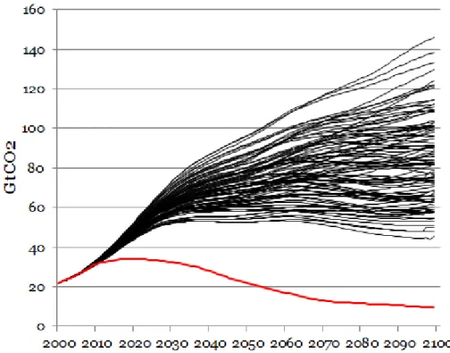
Figure 1: Global emissions over the century in the 96 simulations without climate policy (each black line corresponds to a scenario) and cap on global emissions when climate
policies are implemented (red line).
Figure 1 shows global emissions over the 21st century in the 96 simulations in the absence of a climate policy (each black line corresponds to one scenario) and the cap on global emissions when climate policies are implemented (red line). Depending on the assumptions made, the reductions in emissions required differ significantly (between 35 and 140 GtCO2 in 2100 relatively to 2000) and therefore require an effort to reduce emissions more or less important. In Europe, reductions in emissions between 2000 and 2050 range from 35% and 60%, with an average of 50%.
4. Results
Here we present results for Europe, one of the regions represented in the Imaclim-R model.
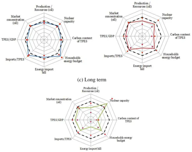
Figure 2: Effects of climate policy on the set of energy security indicators, for Europe, at three time horizons: short-term (mean effect over a five year period centered on 2025), medium-term (mean effect over a five year period centered on 2050) and long-term (mean effect over a five year period centered on 2075). The effect is calculated as the ratio of the value of the indicator in a climate policy scenario to its value in the corresponding baseline, at the same date. The bold line represents the average effect across scenarios; red dots correspond to the 10th and 90th percentiles. The dashed line shows the point at which the ratio would be equal to 1, i.e. where climate policies would not change the value of the energy security indicator. Results outside this line correspond to a worsening of the energy security indicator due to climate policies, while results inside this line correspond to an improvement of the energy security indicator.
(a) Short term (b) Medium term
(c) Long term
Figure 2 shows the effects of climate policy on the set of energy security indicators chosen at three time horizons: short-term (mean effect over a five year period centered on 2025), medium-term (mean effect over a five year period centered on 2050) and long-term
(mean effect over a five year period centered on 2075). The effect is calculated as the ratio of the value of the indicator in the climate policy scenario to its value in the corresponding baseline, at the same date. This is therefore a comparison between two future values of the indicator (the value it would take at a given date in a world where climate policy is implemented vs. the value that it would take at that same future date in a world with no climate policy), of which at least one will not be realized. Comparison with today’s value of the indicator (instead of with the value it would take in a baseline scenario at a future date) would give a different picture.
Note that the axes in Figure 2 are not comparable, i.e. the variation in one indicator cannot be compared with that of another indicator (e.g. it would not make sense to try and compare a 20% drop in the household energy budget with a 20% reduction in the Imports/TPES ratio). This is a common limitation to multi-dimensional evaluations.
4.1.The indicator matters
Figure 2 shows that any conclusion concerning future changes in energy security will depend on the indicator considered: ambitious climate policy improves some indicators and worsens others. In particular the short-term picture entails significant trade-offs.
Another striking result is that for each dimension, the two indicators chosen evolve in opposite directions in the short term. For instance, the energy intensity of the GDP is improved in all scenarios (the two red dots are inside the bold line4), whereas the share of imports in European TPES is increased in all scenarios (the two red dots are outside the bold line4). This result can be explained by:
• The price of carbon makes energy more expensive, at least in the short term before technical change and learning mechanisms have had time to transform the installed productive capacities and equipment, which triggers improvement in energy and structural change, thus reducing the energy intensity of GDP.
• The share of imports in European TPES increases in the short-term because the price of carbon triggers substitution away from (mainly domestic) coal toward (mainly imported5) gas in power generation and end-use efficiency. The substitution is mainly toward gas and less toward renewable energies because at low carbon prices, renewable energies are less competitive for the generation of power than gas. The assumption of myopic anticipation of carbon prices in the Imaclim-R framework exacerbates this result. Considering perfect anticipation of future carbon prices would moderate this result and trigger more renewable and less gas penetration in the short term. A shale-gas ”revolution” in Europe could also change this result, but the reproduction of the United States experiment faces several barriers (Cherp et al. (2012), Box 5.5), including different geology, a more sensitive natural and cultural environment, etc. For that reason, large scale extraction of shale gas in Europe in the short term is not included in our scenarios.
Consequently, depending on the indicator used, conclusions concerning the dependence dimension of the energy security can be opposed. This explains the sometimes contradictory conclusions in the literature and reveals the importance of analyzing not only all the dimensions of energy security but also the different aspects of each dimension.
4 This means that the result holds for the 10th and 90th percentiles. It is in fact also true for extremes. 5 In Europe, in 2011, imports of coal amounted to 30% of total primary coal supply, while gas imports
4.2.Time horizon matters
Another result is that time matters: the effects of climate policy on the set of energy security indicators differs considerably depending on the time horizon considered. Climate policy can have a negative effect on an indicator in the short term but improve it later. Moreover, while the short term is characterized by many trade-offs, the medium- and long term reveal deterioration of only one or two indicators. Nevertheless, the further the horizon, the greater the range of uncertainty on the results. It can thus be seen that:
• In all scenarios and at all time horizons, three indicators improve when climate policies are implemented: the ratio of oil production to resources, the energy intensity of GDP (TPES/ GDP) and the carbon content of energy. We have already explained why the energy intensity of GDP is improved. In the same way, by putting a price on carbon, climate policy triggers substitutions away from carbon intensive energy sources, thus reducing the carbon content of the energy mix and economic activity in fossil intensive sectors, in particular in oil intensive sectors; therefore the ratio of oil production to resources is improved6.
• One indicator, the households’ energy budget, is worsened by climate policy in the short term, but on average, improves in the medium and long terms, although with some cases of persistent deterioration. The short-term degradation of the households’ energy budget is due to higher energy prices (due to the carbon price) and inertia in adapting stocks of energy-consuming equipment to these higher prices. But learning mechanisms and improvements in end-use efficiency explain why the worsening is only transitory. Similarly, learning and changes in the energy generation mix explain why the increase in electricity prices due to the carbon prices can be only transitory; hence households do not necessarily face higher energy prices for the whole time horizon. Cases of persistent deterioration of the households’ energy budget correspond to scenarios with a combination of low availability of low carbon end-use technologies, such as electric vehicles and efficient buildings, and relatively abundant fossil fuels (which leads to moderate energy prices in the baseline). • The share of imports in TPES increases in the short term, but, on average, improves in the medium term and in all scenarios in the long term. In the short term, the move away from (partly domestic) coal to (mainly imported) gas increases the share of energy imports. But, over the medium and long terms, the increasing share of renewable energies in the energy mix allows a reduction in imports.
• The concentration of oil markets (equivalent to the diversity of oil imports in our framework since imports are not modeled bilaterally but via an international pool) deteriorates on average and in most cases in the short and medium terms but is improved in the long term. Climate policy restricts the extraction of unconventional oil due to lower demand, which limits the range of producers. This result corroborates findings by Kruyt et al. (2009). In the long term, some conventional oil remains in the climate policy scenarios and maintains more diversity than in baseline cases.
• On average and in most scenarios, the energy import bill as a share of GDP is reduced by climate policies at all time horizons, but the results vary widely across scenarios. This indicator is complex to interpret because its variation depends on the interplay between the effects of climate policies on (i) the volume and structure of energy imports among energy types, (ii) international energy prices and (iii) GDP.
6 Exploration is not modeled in our framework, so total resources are exogenous, while the resources
In the short term, climate policy increases the amount of imported gas and reduces the amount of imported coal and oil. The international price of gas then increases, while the international prices of oil and coal decrease. Climate policy also reduces GDP compared to baseline values. The effect on oil and coal tends to dominate, which explains the decrease in the energy import bill as a share of GDP on average over in the short term.
In the medium term, the reduction in international energy prices (due to less demand) is the main factor that explains the reduction in the energy import bill. In the long term, the range of uncertainty is very broad, but the net effect is always a reduction in the import bill.
• The installed nuclear capacities follows more complex time trends, with, on average, a deterioration in the short term, an improvement in the medium term and a new deterioration in the long term. It is also characterized by large uncertainties and cases of both improvement and worsening can be found at all three time horizons. The effect of climate policies on installed nuclear capacities results from the combination of conflicting mechanisms. Substitutions in the power generation mix tend to increase the share of nuclear capacities. But electricity production can either increase or decrease: energy efficiency in end uses reduces demand but substitutions between energy types tend to increase electrification of end uses, hence increasing demand. The overall effect is ambiguous and depends on the relative weights of these conflicting forces.
4.3.Uncertainty matters
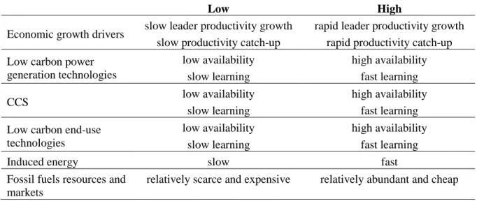
The full analysis of the effects of uncertainties on the different sets of model parameters on the results (that we call determinants in the remainder of this section) is beyond the scope of a single article. But our scenarios database made it possible to explore the role played by the different determinants of the energy security indicators. We compare the effects of the climate policy on the indicators depending on whether the assumption concerning the determinant is “low” or “high” (Table 2).
Table 2: Definition of “low” and “high” alternative assumptions for the six uncertainties considered in the scenario database
Low High
Economic growth drivers slow leader productivity growth
slow productivity catch-up
rapid leader productivity growth rapid productivity catch-up Low carbon power
generation technologies low availability slow learning high availability fast learning CCS low availability slow learning high availability fast learning Low carbon end-use
technologies
low availability slow learning
high availability fast learning
Induced energy slow fast
Fossil fuels resources and markets
relatively scarce and expensive relatively abundant and cheap
Here, we limit our analysis to the medium term. Results for short and long terms can be seen in Appendix C.
For each energy security indicator and each determinant, Figure 3 shows the average effect of climate policies on the value of the indicator in the two subsets of the scenarios database: those where the determinant is low (in blue), and those where the determinant is high (in red).
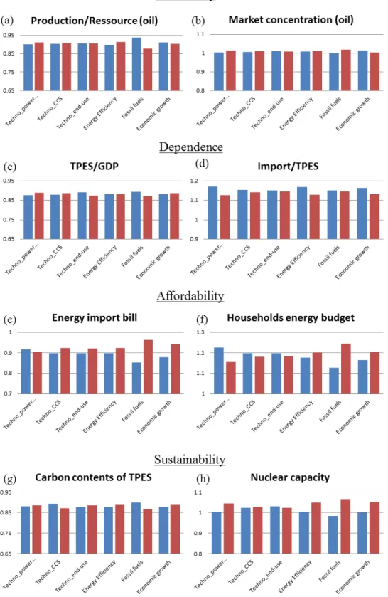
For most indicators, the direction of the average effect of climate policy is not altered by a “low” or “high” assumption for a given determinant (for most determinants, blue and red bars are either both below 1 or both above 1 in Figure 3). The main exception is the share of imports in TPES: climate policy improves or worsens the indicator depending on the availability of low carbon technologies (for electricity production and for CCS) or on the intensity of the induced energy efficiency. Indeed, high availability of CCS or of low carbon power generation technologies makes it possible to limit imports without requiring a major reduction in TPES. Assumptions on induced energy efficiency have more effect on the denominator of the imports to TPES ratio, i.e. a “high” assumption causes a drop in TPES, which has a negative effect on the indicator. Another exception is the installed nuclear capacity, which is increased by climate policies when the assumption on power generation technologies is “high” (relatively high potentials and low costs of low carbon technologies) whereas it is reduced when the assumption on power generation technologies is “low” (relatively low potentials and high costs of low carbon technologies). But this result is in a way tautological because the assumption on power generation technologies includes assumptions on the cost of nuclear plants and maximum shares in the generation mix.
For other indicators, the conclusion concerning the effect of climate policy is not reversed when a specific assumption is changed, but the value of the ratio may change considerably. Moreover, none of the determinants has its effects in the same direction for all the indicators. For each determinant, some indicators are improved when the determinant is “high” (the red bar is below the blue bar), but at the same time, some indicators are worsened (the red bar is above the blue bar).
• Assumptions on low carbon power generation technologies influence the indicators of the dependence and sustainability dimensions but less the indicators of availability and affordability dimensions.
• Assumptions on CCS technology play an important role in the energy intensity of GDP, the share of imports in TPES, the households’ energy budget and carbon content of TPES, but a relatively less important role in the other indicators. The relatively high availability and low cost of this technology limit the reduction in the TPES when climate policy is implemented, which increases the TPES to GDP ratio and decreases the imports to TPES ratio. The relatively low cost of CCS also has a positive impact on the households’ energy budget because decarbonization happens at a relatively lower carbon tax. For the same overall emissions, when CCS is cheaper, TPES is less reduced by climate policy, but the carbon to TPES ratio (calculated after deduction of emissions captured and sequestrated) is more reduced.
• Assumptions on low carbon end-use technologies have only a moderate impact compared to other determinants. The most affected indicator is nuclear capacity. The different technologies considered lead to both a decrease in energy demand and the electrification of end uses. When the assumption is “high”, the overall effect is an increase in electricity demand, which leads to more installed nuclear capacity.
• On average, the cases of fast induced energy efficiency have a strong negative effect compared to the cases of slow induced energy efficiency for several indicators: the oil market concentration, the import share of TPES, the energy import bill, as well as the carbon content of TPES. The somewhat surprising negative effect of fast induced energy efficiency can in fact be explained: since climate policy is modeled with a fixed objective of
emission trajectory, the more rapid the induced energy efficiency (in end uses in agriculture, industry, construction and services), the less the emission reduction efforts depend on supply, hence the negative effect on indicators of energy security with respect to the supply side.
• Assumptions on fossil fuels have a relatively strong effect on most of the indicators. The impact of highly abundant fossil fuels is obviously positive for the indicators of the availability dimension. Climate policy also improves the energy intensity of GDP more in the case of abundant fossil fuels, simply because this intensity is higher in the baselines in which economic development depends on relatively cheap and abundant fossil fuels. The effect is also positive on the share of the energy import bill in the GDP: the effect of the reduction in the import volumes of energy dominates. On the contrary, it negatively impacts the households’ energy budget. The abundance of fossil fuels leads to moderate energy prices in the baselines. Consequently, in order to limit the consumption of fossil fuels, climate policy requires a higher carbon tax, which will inflate the household energy budgets. • Lastly, the assumptions on the drivers of the economic growth are of moderate importance for the ratio of oil production to resources and oil market concentration. The effects are opposite. When economic growth is rapid, more resources are extracted in the baseline scenario. Hence, the limitation of extraction due to climate policy is relatively more important, and the oil production to resources ratio is better. But when economic growth is rapid, there is larger and faster penetration of unconventional fuels in the baseline, and therefore more diversification of oil producers (than in the baselines with relatively slower growth); climate policy hinders such penetration, hence prohibiting diversification.
Figure 3: Average effect of climate policies in the medium term (mean effect over a five year period centered on 2050) on the indicator value for two subsets of the scenarios database: those in which the determinant is low (in blue), and those in which the determinant is high (in red). The effect is calculated as the ratio of the value of the indicator in a climate policy scenario to its value in the corresponding baseline. As before, a ratio of less than 1 represents an improvement in the indicator due to the climate policy, while a ratio of more than 1 represents a worsening of the indicator.
5. Conclusion
This article presents a methodology to investigate whether climate policy would improve energy security, accounting for the difficulties entailed by the many-faceted nature of the energy security concept and the large uncertainties on the determinants of future changes in energy systems. The method uses a set of indicators in a four-dimension analysis grid of the energy security concept, and a database of scenarios to explore the uncertainty space.
Any analysis based on the use of indicators and of scenarios is necessarily based on a number of simplifications. The one reported on this article is no exception to this rule. It would be interesting to analyze other indicators, such as the ratio of production to resources and the diversity of producers in the case of other fuels than oil. Other scenario variants could also be relevant.
Nevertheless, the results we present here focusing on Europe, highlight several messages that have important policy implications. First, there is no unequivocal effect of climate policy on all the dimensions of the energy security and some trade-offs are involved. The many-faceted nature of energy security matters: energy security has several dimensions, and some can be worsened by climate policy. Time matters: the effect of climate policy on energy security depends on the time horizon considered. Last, these results are robust to key uncertainties on the future potential and costs of technologies, on future improvements in energy efficiency, on fossil fuel resources and markets and on drivers of economic growth. However, some of these uncertainties determine the magnitude of the effect of climate policy on energy security indicators.
Our results enable the identification of some risks of contradiction between climate objectives and energy security, and suggest when complementary policies may be necessary to reconcile the two objectives. In particular, there is a risk that climate policy may reduce the affordability of energy for households in the short term. Measures that target modest households could therefore be included in the policy package to moderate trade-offs.
Moreover, gas plays an important role in reducing short-term carbon emissions, because low carbon prices trigger substitution toward gas, and not so much toward zero-carbon technologies. Therefore, climate policies may reduce European energy independence (its share of imports in TPES in particular). This may justify considering complementary policies in favor of zero-carbon technologies to limit the role of gas in the transition to a low-carbon economy. Otherwise, measures to secure the supply of gas will be required.
Further research is needed to investigate more detailed climate policy designs than the extremely stylized one considered in this article. It would be interesting to analyze how results change under unilateral climate policies or fragmented climate policy regimes, for other instruments than a carbon price, or for different levels of climate policy ambitious. Comparisons of results obtained for other regions would provide additional insights.
References
Armington, P. S., 1969. A theory of demand for products distinguished by place of production. Staff Papers, International Monetary Fund 16 (1), 159–178.
Brown, S., Huntington, H. G., 2008. Energy security and climate change protection: Complementarity or tradeoff ? Energy Policy 36 (9), 3510–3513.
Cherp, A., Adenikinju, A., Goldthau, A., Hernandez, F., Hughes, L., Jansen, J., Jewell, J., Olshanskaya, M., Soares de Olilveira, R., Sovacool, B., Vakulenko, S., Bazilian, M., Fisk, D. J., Pal, S., 2012. Energy and security (chapter 5). In: Global Energy Assessment, Toward
Chester, L., 2010. Conceptualising energy security and making explicit its many-faceted nature. Energy policy 38 (2), 887–895.
Corrado, C., Mattey, J., 1997. Capacity utilization. The Journal of Economic Perspectives 11 (1), 151–167.
Dimaranan, B., McDougall, R. A., 2006. Global Trade, Assistance and Production: The GTAP 6 Data Base, Center for Global Trade Analysis. Purdue University, West Lafayette, IN.
European Commission, 2001. Towards a European strategy for security of energy supply. European Union, 2011. Communication from the commission to the European parliament, the council, the European economic and social committee and the committee of the regions energy roadmap 2050.
Grubb, M., Butler, L., Twomey, P., 2006. Diversity and security in UK electricity generation: The influence of low-carbon objectives. Energy Policy 34 (18), 4050–4062. Hartley, P. R., 2008. Climate policy and energy security: two sides of the same coin? Ph.D. thesis, Department of Economics, Rice University.
IEA, 2007. Energy Security and Climate Policy, Assessing Interactions, OECD/IEA Edition. Paris.
IEA, 2013. Energy Statistics of OECD countries, 2013 Edition, IEA Edition. IEA Statistics. Paris.
Kirton, J., 2007. The G8’s energy-climate connection. In: Workshop or Talking Shop? Globalization, Security and the Legitimacy of the G8. Brussels.
Kruyt, B., Van Vuuren, D. P., De Vries, H. J. M., Groenenberg, H., 2009. Indicators for energy security. Energy Policy 37 (6), 2166–2181.
Kuik, O., 2003. Climate change policies, energy security and carbon dependency trade-offs for the european union in the longer term. International Environmental Agreements: Politics, Law and Economics 3 (3), 221–242.
Maisonnave, H., Pycroft, J., Saveyn, B., Ciscar, J. C., 2012. Does climate policy make the EU economy more resilient to oil price rises? a CGE analysis. Energy Policy 47, 172-179. McCollum, D. L., Krey, V., Riahi, K., 2011. An integrated approach to energy sustainability. Nature Climate Change 1 (9), 428–429.
McCollum, D. L., Krey, V., Riahi, K., Kolp, P., Grubler, A., Makowski, M., Nakicenovic, N., 2012. Climate policies can help resolve energy security and air pollution challenges. Climatic Change, 1–16.
O’Neill, B. C., Kriegler, E., Riahi, K., Ebi, K. L., Hallegatte, S., Carter, T. R., Mathur, R., van Vuuren, D. P., 2013. A new scenario framework for climate change research: The
Rozenberg, J., Hallegatte, S., Vogt-Schilb, A., Sassi, O., Guivarch, C., Waisman, H., Hourcade, J. C., 2010. Climate policies as a hedge against the uncertainty on future oil supply. Climatic Change, 1–6.
Rozenberg, J., Guivarch, C., Lempert, R., Hallegatte, S., forthcoming. Building SSPs for climate policy analysis: a scenario elicitation methodology to map the space of possible future challenges to mitigation and adaptation. Climatic Change.
Sassi, O., Crassous, R., Hourcade, J.-C., Gitz, V., Waisman, H., Guivarch, C., 2010. IMACLIM-R: a modelling framework to simulate sustainable development pathways. International Journal of Global Environmental Issues 10 (1), 5–24.
Schafer, A., Victor, D. G., 2000. The future mobility of the world population. Transportation Research Part A 34 (3), 171–205.
Schlesinger, R., 1989. Energy and geopolitics in the 21st century. Montreal, Canada.
Sovacool, B. K., Brown, M. A., 2010. Competing dimensions of energy security: An international perspective. Annual Review of Environment and Resources 35, 77–108.
Turton, H., Barreto, L., 2006. Long-term security of energy supply and climate change. Energy Policy 34 (15), 2232–2250.
van Vliet, O., Krey, V., McCollum, D., Pachauri, S., Nagai, Y., Rao, S., Riahi, K., 2012. Synergies in the asian energy system: Climate change, energy security, energy access and air pollution. Energy Economics 34 (S3), S470-S480.
Waisman, H., Guivarch, C., Grazi, F., Hourcade, J., 2012. The Imaclim-R model: infrastructures, technical inertia and the costs of low carbon futures under imperfect foresight. Climatic Change 114 (1), 101–120.
Appendixes
A. Description of the scenarios database
A.1. Drivers of economic growth
The natural growth rate of the economy defines the growth rate that the economy would follow if it produced a composite good at full employment, like in standard neoclassical models developed after Solow (1956). Equation 1 represents labor productivity growth through the decrease in unitary labor input l in each region j and at each time step t.
( )
1( )
1( ) (
) (
)
0 2 , , 1 , , , t t t l t j e τ l t j e τ l t j l t leader l t leaderτ
− − = ⋅ + − ⋅ ⋅ − + i i (1)In line with the SSP quantifications, we build assumptions combining hypotheses on population growth, on the leader productivity growth, and on catch-up speed for two groups of regions: high income and low income countries (see Tables 3 and 4).
Table 3: Parameters options for leader growth and high income population growth. Population data are available at https://secure.iiasa.ac.at/web-apps/ene/SspDb
Slow growth Intermediate growth Rapid growth
Leader productivity growth slow medium rapid
High income population growth SSP3 SSP2 SSP1
Table 4: Parameters options for low income catch-up speed and population growth. Population data are available at https://secure.iiasa.ac.at/web-apps/ene/SspDb
Slow growth Intermediate growth Rapid growth
Low income catch up time (τ2 in eq. 1, in
years) 300 200 150
Low income population growth SSP3 SSP2 SSP1
A.2. Availability of different types of low carbon technologies
In the Imaclim-R model, technologies penetrate the markets according to their profitability, but are constrained by a maximum market share which follows a S-shaped curve (Grubler et al., 1999). We consider two alternatives for each group of technologies. The high availability assumption corresponds to an earlier start date (only for Carbon Capture and Storage), a higher maximum market share, and faster diffusion than under the low availability assumption. Moreover, for some new technologies, there is an endogenous learning mechanism: the cost of the technology is reduced with the cumulative investment in that technology. This mechanism is governed by a learning rate, and two alternative values are considered for this learning rate.
• Low carbon power generation technologies
The technologies considered are nuclear and renewable energies. In the low availability assumption it is assumed that the new generation of nuclear energy is not available at all. The parameters are described in Table 5.
• Carbon Capture and Storage (CCS)
The parameters of each alternative are listed in Table 5. • Low carbon end-uses technologies
The technologies considered are electric and hybrid vehicles, efficient buildings and household equipment. The parameters for electric and hybrid vehicles are described in Table 5.
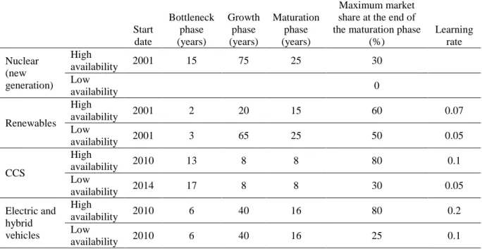
Table 5: Parameters options for low carbon power generation, CCS and electric and hybrid vehicles Start date Bottleneck phase (years) Growth phase (years) Maturation phase (years) Maximum market share at the end of the maturation phase
(%) Learning rate Nuclear (new generation) High availability 2001 15 75 25 30 Low availability 0 Renewables High availability 2001 2 20 15 60 0.07 Low availability 2001 3 65 25 50 0.05 CCS High availability 2010 13 8 8 80 0.1 Low availability 2014 17 8 8 30 0.05 Electric and hybrid vehicles High availability 2010 6 40 16 80 0.2 Low availability 2010 6 40 16 25 0.1
In the residential sector, the buildings stock is divided into two types of buildings: “classical” buildings and very low energy buildings (that consume 50 kWh per square meter and per year, 80% of which is electricity and 20% gas). The energy consumption of “classical” buildings is described by equation 2. The penetration of very low energy buildings depends on its extra investment cost that decreases following a learning rate. The parameters are listed in Table 6.
Housing energy expenditure of “classical” buildings:
( )
(
2)
e Exp h m stock e e H =∑
µ t ⋅α ⋅b ⋅pFD (2)where HExp is the total energy expenditure in housing, for each country; 2
e m
α is the energy consumption of buildings e per m2, in each country (exogenous trend calibrated on POLES: see LEPII-EPE (2006));
µ
h( )
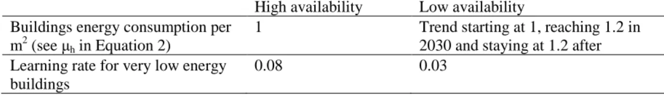
t is a multiplier coefficient at year t; bstock is the building stock in each country; pFDe is the price of final demand for energy e in each country (which takesTable 6: Parameters options for residential buildings and household equipment
High availability Low availability
Buildings energy consumption per m2 (see µh in Equation 2)
1 Trend starting at 1, reaching 1.2 in
2030 and staying at 1.2 after Learning rate for very low energy
buildings
0.08 0.03
A.3.Induced energy efficiency
In each sector, the country with the lowest energy intensity is the leader and its energy efficiency is triggered by energy prices. After a delay, the other countries catch up with the leader. We build two hypotheses (see Table 7) using the following parameters: maximum annual improvement in the leader’s energy efficiency, other countries’ speed of convergence (% of the initial gap after 50 years) and asymptotic level of catch up (% of the leader’s energy efficiency).
Table 7: Parameters options for energy efficiency
Fast Slow
Maximum annual improvement in the leader’s energy efficiency 1.5 0.7
Other countries speed of convergence (% of the initial gap after 50 years) 10 50
Asymptotic level of catch-up (% of the leader’s energy efficiency) 95 60
A.4. Fossil fuels - resources and markets A.4.1. Oil
The modeling structure of oil supply in Imaclim-R is based on three general principles. First, a physical description of oil resources with an explicit differentiation according to the region and nature (conventional vs. non- conventional) is used in the dynamic submodel to describe changes in oil producing capacities (see Equation 3). Oil resource availability is based on data from USGS (2000); Greene et al. (2006) and Rogner (1997). Secondly, an explicit differentiation is made between fourteen (seven conventional and seven non-conventional) categories of resources in each region according to the cost of exploration and exploitation. As oil must be discovered before it is produced, the temporal availability for production of a given category of oil resources depends on the characteristics of the discovery process, which is subject to two main effects: the information effect (the more an oil slick is exploited, the more information about the localization of remaining resources is obtained) and the depletion effect (the more a slick is exploited, the less oil remains in the soil). Following Rehrl and Friedrich (2006), inertias in the deployment of oil producing capacities resulting from the combination of these technical constraints on the discovery process are captured through independent bell-shaped curves that determine the changes in the oil producing capacities over time for each category of oil in each region.
We distinguish the different categories of regional oil resources according to their production costs (i.e. including exploration and exploitation costs) and the nature of the resource (conventional or non-conventional). To this end, we associate a bell-shaped time profile of its production with each resource category:
( ) ( )
(
)
0 0 2 1 b t t b t t Q b e e − − ∞ − − ⋅ ⋅ + (3)where t is the current date, t0 is the starting date of oil production for this category, Q∞is the
amount of ultimate resources and b is a parameter that captures the intensity of constraints that slow down production growth.
Concerning the dynamics of production capacities, Imaclim-R distinguishes two types of oil producers according to their investment behaviors. All non-Middle-Eastern countries are assumed to be motivated by short-term returns on investments, which implies that they will bring a category of oil reserve into production as soon as it becomes profitable (that is when the selling price on world market exceeds the total cost of exploration and exploitation). From then on, the deployment of production capacities is limited by geological constraints and strictly follows the corresponding bell shaped curve. Producers who do not use any strategic behavior are referred to as “fatal producers” (Rehrl and Friedrich, 2006). The situation is different for Middle Eastern producers, as the amount of their oil resource gives them market power and allows them to choose a strategy to fulfill a specific objective (either a price or a market share target). For a given year, Middle Eastern production capacity is still bounded by a bell-shaped curve but its actual production may be below this limit if the chosen strategy requires a restriction on production. This “swing producer” (Rehrl and Friedrich, 2006) behavior is consistent with past OPEC production, which has not fitted the discovery trend since the oil shocks in the 1970s (Laherrere, 2002).
Middle Eastern countries can use their market power in two opposite ways (and any combination in between). The first is to secure high prices in the short run by limiting the expansion of their production capacities; but this strategy has the disadvantage of encouraging oil importing countries to accelerate their efforts to develop oil free technologies and to adopt energy-sober consumption patterns. The second one is a “market flooding” strategy to maintain rather low prices in the short-term to encourage oil consumption and discourage oil importing countries from continuing efforts to save oil. The trade-off is between low revenues in the coming decades and higher income in the long run, the lower price elasticity of the oil demand being due to the lack of large scale cheap substitutes for oil. The trade-off between these two assumptions does not depend only on the flows of export revenues, it also depends on geopolitical considerations and on the long term objectives of the Middle Eastern governments, including the way they prepare their “post-oil” era. The conduct of these strategies will depend on the internal agreement among OPEC members and Middle Eastern countries. When OPEC countries agree on policy, they may agree to cut back production so that oil prices are high; conversely, when they are divided, they tend to produce more individually, resulting in lower oil prices.
Within this oil supply module, we decided to explore the uncertainty on the components of three major parameters to describe different levels of oil scarcity: the amount of ultimately recoverable resources, the level of inertia that will shape the development of non-conventional production, and the OPEC target oil price (see Table 8).
A.4.2. Gas
In the model, gas world production capacities match demand growth until ultimately recoverable resources enter a depletion process. Variations in gas prices are indexed on variations in oil prices via an indexation coefficient (0.68, see Equation 5) calibrated on the
World Energy Model (IEA, 2007). When oil prices increase by 1%, gas prices increase by 0.68%.
Two alternative assumptions are used in this price indexation. Under the assumption “relatively abundant and cheap” for the fossil fuel resources and market parameter set, this indexation disappears when oil prices reach 80$/bl: beyond this threshold, fluctuations in gas prices only depend on production costs and possibly on the depletion effect. When depletion is reached, price increases. Under the assumption “relatively scarce and expensive”, gas prices remain indexed on oil prices regardless of fluctuations, but an additional price increase occurs when gas production enters its depletion phase.
The price of gas in each region at year t is:
( )
ref( )
gas gas gas
p t = p ⋅
τ
t (4)where pgasref is the gas price in this region at year 1.
As long as gas depletion has not started, τgas(t) in each region is:
( )
1( )
2( )
10.68 1
3 3
gas oil oil ref
oil
t wp t wp t
wp
τ
= ⋅ ⋅ + ⋅ − ⋅ (5)
Where wpoil(t) is the world oil price at year t; wpoilref is the world oil price at year 1.
If depletion has started in this region, τgas(t) increases 5% each year, regardless of oil prices.
A.4.3. Coal
Coal is treated in a different way than oil and gas because more coal resources are available, which prevents coal production from entering a depletion process before the end of the 21st century.
We describe price formation on the world coal market in a reduced functional form linking variations in price to variations in production. This choice allows us to capture the cyclic behaviour of this commodity market. Coal prices then depend on current production through an elasticity coefficient ηcoal: tight coal markets exhibit a high value of ηcoal (i.e. the
price of coal increases if coal production increases). We make two assumptions for ηcoal (see
Table 8). Under the assumption of “relatively abundant and cheap” the sensitivity of an increase in coal price to an increase in coal production is quite low, so that the increase in coal production can be absorbed without price fluctuations. Conversely, the increase in coal price is very sensitive to any increase in coal production under the assumption “relatively scarce and expensive”.
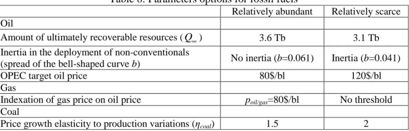
Table 8: Parameters options for fossil fuels
Relatively abundant Relatively scarce
Oil
Amount of ultimately recoverable resources (Q∞) 3.6 Tb 3.1 Tb
Inertia in the deployment of non-conventionals
(spread of the bell-shaped curve b) No inertia (b=0.061) Inertia (b=0.041)
OPEC target oil price 80$/bl 120$/bl
Gas
Indexation of gas price on oil price poil/gas=80$/bl No threshold
Coal
References
Greene, D. L., Hopson, J. L., Li, J., Mar. 2006. Have we run out of oil yet? oil peaking analysis from an optimist’s perspective. Energy Policy 34 (5), 515–531.
Grubler, A., Nakicenovic, N., Victor, D. G., May 1999. Dynamics of energy technologies and global change. Energy Policy 27 (5), 247–280.
IEA, 2007. World energy outlook. Tech. rep., IEA/OECD, Paris, France.
Laherrere, J., 2002. Forecasting future production with past discoveries. International Journal of Global Energy Issues 18 (2-4), 218-238.
LEPII-EPE, 2006. The POLES model, POLES State of the Art. Institut d’économie et de Politique de l’énergie, Grenoble, France.
Rehrl, T., Friedrich, R., 2006. Modelling long-term oil price and extraction with a hubbert approach: The LOPEX model. Energy Policy 34 (15), 2413–2428.
Rogner, H., 1997. An assessment of world hydrocarbon resources. Annual review of energy and the environment 22, 217–262.
Solow, R. M., 1956. A contribution to the theory of economic growth. Quarterly Journal of Economics 70, 65–94.
USGS, 2000. World petroleum assessment 2000. Tech. rep., United States Geological Survey, USA, Washington.
B. Regional and sectoral aggregation of Imaclim-R model
Regions Sectors
• USA, • Canada, • Europe,
• Pacific OECD (Japan, Australia, New-Zealand, South Korea), • Commonwealth of Independent States, • China, • India, • Brazil, • Middle East, • Africa, • Rest of Asia,
• Rest of Latin America.
• Coal, • Oil, • Gas,
• Liquid fuel refinery, • Power generation, • Air transportation,
• Maritime and water transportation, • Terrestrial transportation,
• Construction, • Agriculture, • Industry,
• Composite sector (services and light industry).
C. Results of uncertainties for the short term and long term
Figure 4: Average effect of climate policies in the short term (mean effect over a five year period centered on 2025) on the indicator value for two subsets of the scenarios database: those in which the determinant is low (in blue), and those in which the determinant is high (in red). The effect is calculated as the ratio of the value of the indicator in a climate policy scenario to its value in the corresponding baseline. As before, a ratio of less than 1 represents an improvement in the indicator due to the climate policy, while a ratio of more than 1 represents a worsening of the indicator.
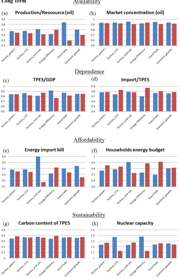
Figure 5: Average effect of climate policies in the long term (mean effect over a five year period centered on 2075) on the indicator value for two subsets of the scenarios database: those in which the determinant is low (in blue), and those in which the determinant is high (in red). The effect is calculated as the ratio of the value of the indicator in a climate policy scenario to its value in the corresponding baseline. As before, a ratio of less than 1 represents an improvement in the indicator due to the climate policy, while a ratio of more than 1 represents a worsening of the indicator.