Extreme meteo-oceanic events

HAL Id: tel-01743728

https://pastel.archives-ouvertes.fr/tel-01743728

Submitted on 26 Mar 2018

HAL is a multi-disciplinary open access

archive for the deposit and dissemination of

sci-entific research documents, whether they are

pub-lished or not. The documents may come from

teaching and research institutions in France or

abroad, or from public or private research centers.

L’archive ouverte pluridisciplinaire HAL, est

destinée au dépôt et à la diffusion de documents

scientifiques de niveau recherche, publiés ou non,

émanant des établissements d’enseignement et de

recherche français ou étrangers, des laboratoires

publics ou privés.

To cite this version:

Franck Mazas. Extreme meteo-oceanic events. Environmental Engineering. Université Paris-Est,

2017. English. �NNT : 2017PESC1148�. �tel-01743728�

pr´

esent´

ee pour l’obtention du grade de

Docteur de l’Universit´

e Paris-Est

par

Franck Mazas

´

Ev`

enements m´

et´

eo-oc´

eaniques extrˆ

emes

Sp´

ecialit´

e : Sciences et techniques de l’environnement

Soutenue le 17 novembre 2017 devant le jury compos´

e de :

Rapporteur

Dr. Xavier Bertin

LIENSs, CNRS - Universit´

e de La Rochelle

Rapporteur

Pr. ´

Eric Gaume

IFSTTAR

Pr´

esidente

Pr. Liliane Bel

AgroParisTech

Examinateur

Pr. Michel Benoit

Ecole Centrale Marseille, Irph´

´

e

Examinateur

Dr. Pietro Bernardara

CEREA, EDF R&D

Examinateur

Dr. Ivan Haigh

University of Southampton

Directrice de th`

ese

Dr. Nicole Goutal

LHSV, EDF R&D

Co-encadrant de th`

ese

Dr. Luc Hamm

ARTELIA

E

X T R EM E M E T EO

-

O C EA N O G R A P HIC E V E N T S

P

. D .

–

F

M A Z A S

S

S

ARTELIA Eau & Environnement 6 rue de Lorraine

38130 - Echirolles

Tel. : +33 (0) 4 76 33 40 00 Fax : +33 (0) 4 76 33 43 33

Sources of illustrations

Cover: Southern Ocean onboard Jérôme Poncet’s Golden Fleece, January 2014, © Nelly Meignié Huber Part 1: Emmanuel Lepage, Voyage aux Îles de la Désolation Part 2: Marin-Marie, Le Pourquoi Pas ? au large de l’Islande

“Ce sont les évènements qui commandent aux

hommes, et non les hommes aux évènements.”

Hérodote

“Watch therefore,

for ye know neither the day nor the hour.”

Matthew, 25:13

“Prognostics do not always prove prophecies; at least

the wisest prophets make sure of the event first.”

Horace Walpole

TABLE OF CONTENTS

CONTEXT AND ACKNOWLEDGEMENTS __________________________________________ E

PART 1 PRESENTATION OF THE RESEARCH WORK __________________________________ 1

PRESENTATION OF THE DATASETS _____________________________________________ 3

1.

AN INTRODUCTION TO METOCEAN EVENTS ___________________________________ 5

1.1.

W

-

? ____________________________________________ 5

1.2.

M

-

,

_____________________ 9

1.2.1. Analyses for engineering ___________________________________________________ 9 1.2.2. A simple definition of risk __________________________________________________ 9 1.2.3. Illustrative examples, at home ______________________________________________ 10

1.3.

P

:

____________________________ 13

1.4.

B

________________________________________ 18

2.

F

_________________________ 23

2.1.

A

-

POT

_______________ 23

2.2.

A

-

-

______________________ 29

2.3.

M

L

E

_______________________________ 31

2.4.

C

__________________________________________________________ 35

3.

EXTREME MULTIVARIATE EVENTS: FROM SAMPLING TO RETURN PERIOD, A MATTER OF

POINT OF VIEW __________________________________________________________ 37

3.1.

E

:

__________________ 37

3.2.

J

:

MULTIVARIATE

_______________________________________________________________ 43

3.2.1. A new classification for multivariate analyses ________________________________ 43 3.2.2. Sampling: a description of events __________________________________________ 44 3.2.3. Dependence: assessment and modelling ____________________________________ 48 3.2.4. Joint distribution: a first interpretation ______________________________________ 49

3.3.

C

________________________________________ 53

3.3.2. Bivariate return period of source variables vs. univariate return periods of

response variables _____________________________________________________________ 55 3.3.3. Return periods and contours _______________________________________________ 56

3.3.3.1. Contours for event-describing values _________________________________________ 56 3.3.3.2. Contours for sequential values ______________________________________________ 59

4.

CONCLUSIONS AND PERSPECTIVES _______________________________________ 67

4.1.

M

__________________________________________________________ 67

4.2.

D

____________________________________________________________ 68

4.3.

P

__________________________________________________________ 69

GLOSSARY _____________________________________________________________ 71

REFERENCES ___________________________________________________________ 73

PART 2 MAIN PUBLICATIONS ________________________________________________ 79

1.

C

___________________________________________ 81

1.1.

C

E

2011:

A

-

POT

____________________________________________ 81

1.2.

N

H

E

S

S

2014:

A

-

-

___________________________ 83

1.3.

O

E

2014:

Q

MLE

EXTREME DISTRIBUTIONS

_______________________________________________________ 85

1.4.

C

E

2014:

A

POT

R

J

P

M

_________________________ 87

1.5.

C

E

2017:

A

-

PROBABILITIES OF WAVES AND SEA LEVELS

_________________________________________ 89

2.

R PACKAGE ARTEXTREME ______________________________________________ 91

2.1.

R

_______________________________________________________ 91

FIGURES

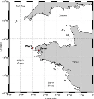
Figure 1. Output point of the WW3 model of Bertin et al. (2013) and location of Brest tide gauge ... 3

Figure 2. Output points Z20A and Z20E for the Groix meteo-oceanic study ... 4

Figure 3. Geographical domains of meteo-oceanography ... 6

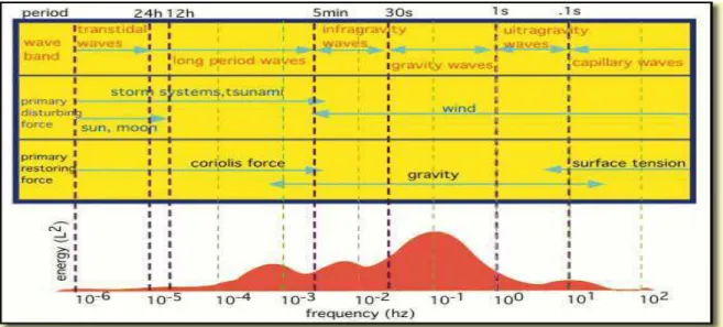
Figure 4. Frequency spectrum of the variations of sea level ... 7

Figure 5. Definition of risk ... 10

Figure 6. Storms of October 1987 and December 1999 (Martin). Top: 500 hPa geopotential height on 16/10/1987 0Z and 27/12/1999 18Z, middle: time series of wind speed (left) and wave height (right) at Brest, bottom: time series of sea level (left) and non-tidal residual (right) at Brest ... 11

Figure 7. Storm Xynthia. Top: 500 hPa geopotential height on 28/02/2010 0Z (left), time series of sea level at La Rochelle-La Pallice tide gauge (right), bottom: time series of sea level, tidal level and non-tidal residual around Xynthia ... 12

Figure 8. La Faute-sur-Mer, hours after the storm peak. In the foreground: the Lay coastal river; in the background: the Atlantic Ocean ... 13

Figure 9. Logo of the OSSË group ... 19

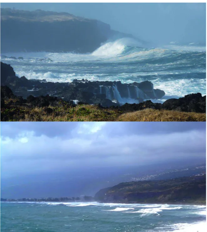
Figure 10. Identification of homogeneous wave populations through the use of directional sectors off Bastia24 Figure 11. Wave populations at Réunion island ... 25

Figure 12. Wave populations at Réunion island. Top: southerly swell in July 2017; bottom: cyclonic waves from tropical storm Chezda in January 2015 ... 26

Figure 13. Fluctuations of the time series of significant wave height ... 27

Figure 14. Stability plot for choosing the high threshold proposed in Mazas and Hamm (2011) ... 28

Figure 15. Plots showing the evolution of the fits to the GPD, Weibull, Gamma and exponential distributions with respect to the threshold: 100-yr Hs quantile (top right), Chi2 statistic (bottom left), p-value of the Kolmogorov-Smirnov test (bottom right) ... 29

Figure 16. Two-step framework for over-threshold modelling, after Bernardara et al. (2014) ... 31

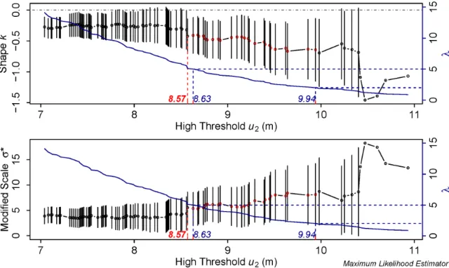
Figure 17. Haltenbanken dataset: change in the ML-estimated GPD shape parameter (top plot, above curve), in 100-yr Hs (top plot, below curve) and in the log-likelihood (down plot, zoom) with respect to the statistical threshold. Dots represent the peak values ... 32

Figure 18. Meteorological virgae ... 33

Figure 19. Change in the ML-estimated vector of GPD parameters _{= , for a simulated dataset of size} 100. True vector of parameters indicated in red. ... 34

Figure 20. Haltenbanken dataset: change in the L-moments estimated GPD shape parameter (top plot, above curve), in 100-yr Hs (top plot, below curve) and in the log-likelihood (down plot, zoom) with respect to the statistical threshold. ... 35

Figure 21. Mean number of sequential values per event with respect to surge height: observations (circles), model (lines). ... 39

Figure 22. Upper tail of the hourly surge values probability density function. ... 40

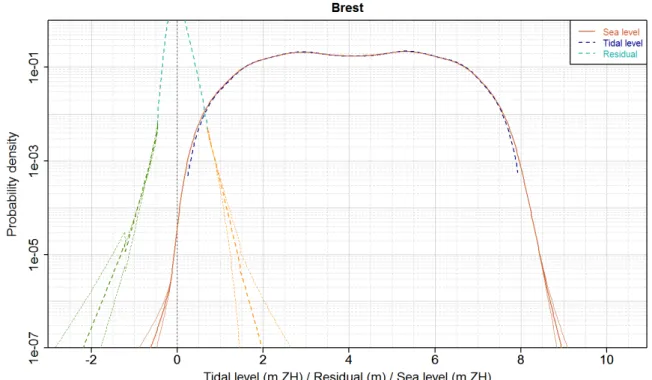
Figure 23. Probability density functions of hourly surge (empirical bulk and parametric tails), astronomical tide and sea level. ... 41

Figure 24. Return periods for sea level events. From the upper to the lower curve: indirect approach without tide–surge interaction, indirect approach with equi-probable tidal bands, indirect approach with equi-probable surge bands, direct approach. ... 42

Figure 25. Illustration of the classification for multivariate analyses ... 44

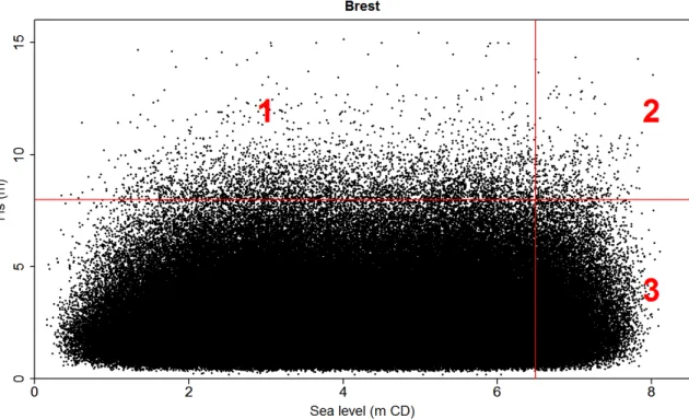
Figure 26. Possible domains for event selection on a Hs / sea level scatterplot ... 45

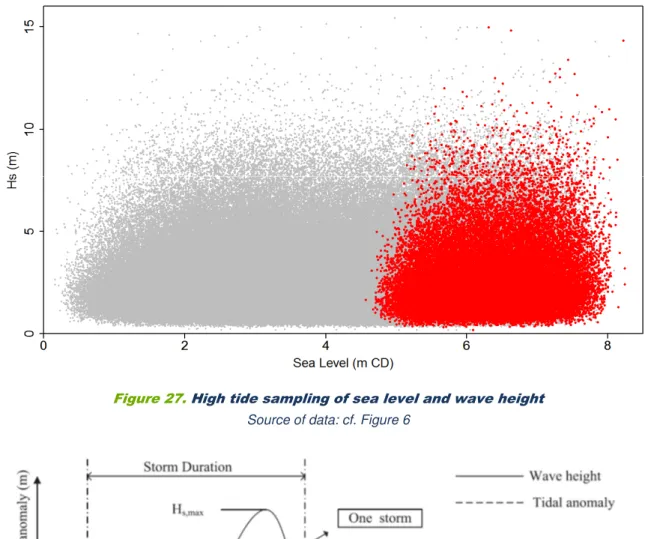
Figure 27. High tide sampling of sea level and wave height ... 46

Figure 29. Top: time series of a univariate response function (sum of sea level and nearshore wave height) with threshold and peak of the selected events; bottom: sequential pairs (Hs, Z) of the time series (in grey)

and selected event-describing pairs (in red) ... 47

Figure 30. Chi-plot (right) for a sample with positive dependence ... 48

Figure 31. Sketch of the bivariate methodology for determining extreme joint probabilities of wave height and sea level ... 49

Figure 32. Comparison of joint return periods between the JOIN-SEA simulations (red dashed lines) and the bivariate methodology (blue plain lines) ... 50

Figure 33. Sketch of the multivariate methodology for determining extreme joint probabilities of wave height and sea level ... 51

Figure 34. Scatterplot sequential values (grey) and event-defining pairs of Hs / sea level (left) and Hs / surge (right)... 51

Figure 35. Modified Hs / surge chi-plot of the i.i.d. sample ... 52

Figure 36. Contours of joint Hs / sea level return periods for the extended bivariate methodology ... 52

Figure 37. Domains and critical regions of several bivariate probabilities ... 54

Figure 38. Joint exceedance probability and structure variable probabilities ... 55

Figure 39. Contours of joint exceedance probabilities and lines of equal univariate return period of the response function (total water level) ... 56

Figure 40. Top: isolines of joint return period; bottom: contours of density associated with extreme Hs for Hs / storm duration bivariate analysis ... 58

Figure 41. Sampling of the Hm0/Tp time series off Groix: scatterplot of the sequential pairs (grey dots) and event-describing pairs (red dots) ... 60

Figure 42. Joint density Hm0/Tp for event-describing pairs ... 61

Figure 43. Parametric domain of the joint distribution for sequential pairs of Hm0 and Tp ... 62

Figure 44. Joint distribution for sequential pairs of Hm0 and Tp ... 63

Figure 45. Contours of sequential Hm0/Tp density associated with extreme Hm0 peaks ... 63

Figure 46. Contours of sequential Hm0/Tp density associated with extreme Hm0 peaks for a homogeneous directional sector ... 64

Figure 47. Contours of sequential Hm0/Ws density associated with extreme Hm0 peaks (top) and extreme wind speed peaks (bottom) ... 65

TABLES

The present document is the supporting statement forming part of the PhD by published works submitted to the École Doctorale SIE (Sciences, Ingénierie et Environnement) of the University of Paris-Est.

The aim of part one is to highlight the consistency of the research work that was undertaken, but also its evolution over the almost ten years it covers. A copy of the main publications is provided in part two.

This work of research began in 2007 during a scientific internship at Sogreah while I was a first-year student at the École Nationale des Ponts et Chaussées (ENPC). The context in which it took place, namely a private engineering company that understood the interest of science and was willing to allocate a fair amount of time and resources to it, was not unrelated to my decision to join the company a couple of years later as an engineer. The research hence steadily kept going, both feeding everyday projects and being fed by them and their ever-increasing technical requirements. This dual dimension of my activity allowed me to be in touch with widely differing communities: colleagues and clients of course, but also members of the national and international scientific community as well as scholars and teachers in the academic world. It was definitely personally and professionally enriching to meet young doctoral students and white-haired scholars during coffee breaks or gala dinners, learn from elder colleagues and teach students from the ENPC and the ESITC, travel the world, and enjoy the life in the Alps.

When it comes to this PhD, I must acknowledge many people. These of course include Dr Luc Hamm who oversaw years of research, enriched it with his scientific mind and advice, and granted me support in the company. And support there was, notwithstanding the changes in organisation and managers: Jacques Viguier, Christophe Peronnard, Sophie Ancel, Alain Deforche and others helped me and allocated resources to enable me to achieve this goal.

In addition to the support he gave to all of his students at the Génie Mécanique et Matériaux department of the ENPC, Dr Alain Ehrlacher was also an early and convincing supporter of developing the research and transforming into a PhD, a position that is not very common in the academic community but that reflects his deep humanity. This warm support was also expressed by many fellow researchers, many of whom are members of the jury. I think particularly of the members of the OSSË working group: Pr Michel Benoit, Dr Pietro Bernardara, Dr Xavier Kergadallan, Marc Andreewsky, Dr Jérôme Weiss, Roberto Frau. I won’t name them here but I think also of many others met at conferences, in particular the “extremers” group of EVAN conferences.

Lastly, personal support and encouragement were also unwavering from my wife Apolline and many friends who know I think of them while writing these words.

P

ART

1

The datasets and results presented in this supporting statement are for illustrative purpose and do not aim at providing quantitative results. Several datasets are also presented in detail in the publications in the second part of this document.

Figure 6, Figure 21 to Figure 27, Figure 29, Figure 32, Figure 34 to Figure 36, Figure 39: atmospheric fields (sea level pressure and 500 hPa geopotential height): archives of ERA-Interim atmospheric reanalyses 0.75°,

wind speed: measurements at Météo-France’s weather station of Guipavas (29),

significant wave height : output point (48.5°N, 5°W, Figure 1) of a 6-hourly database of sea states over the period 1948-2012 from a numerical model built with the WaveWatch III code forced over the Atlantic Ocean by NCEP wind fields and run with the European “Cycle 4” parameterization (Bertin et al., 2013), linearly interpolated every 1 hour,

sea level: hourly measurements at SHOM’s Brest tide gauge (4.4950°W, 48.3829°N,

Figure 1), referenced to the local Chart Datum Zéro Hydrographique 1996, from 1953/01/01 to 2010/12/31 (58 years), corrected of the eustatic trend of + 1.48 mm/yr so as to get a mean sea level of + 4.14 m ZH,

residual: non-tidal residual (considered as the meteorological surge) after removal of the astronomical retro-predictions computed by SHOM’s software SHOMAR;

Figure 1. Output point of the WW3 model of Bertin et al. (2013) and location of Brest tide gauge

Figure 7:

atmospheric fields (sea level pressure and 500 hPa geopotential height): GFS 1° Europe, run 18Z of 2010/02/27,

sea level: measurements at SHOM’s tide gauge of La Rochelle – La Pallice, referenced to the local Chart Datum Zéro Hydrographique,

tidal level: astronomical retro-predictions computed by SHOM’s software SHOMAR, residual: non-tidal residual (considered as the meteorological surge) after removal of the astronomical component from the sea level;

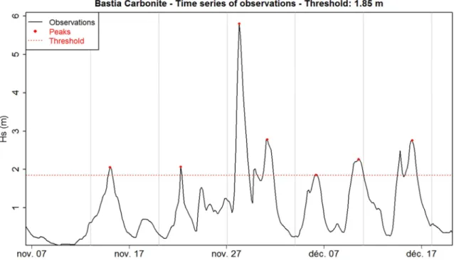
3-hourly numerical modelling of sea states by a WaveWatch III / SWAN coupled model off Bastia’s Carbonite port (~ 450 m deep), run by GlobOcean for ARTELIA;

Figure 14, Figure 17, Figure 19, Figure 20:

Haltenbanken’s dataset of storm peaks of provided by the IAHR Working Group on Extreme Wave Analysis (van Vledder et al., 1994), issued from the analysis of 3-hourly

wave measurements on the Norwegian continental shelf at the deep water locations of 65°05’N, 7°34’E (280 m deep, March 1980 to October 1987) and 65°11’N, 7°15’E (290 m deep, November 1987 to March 1988);

Figure 40:

1992-2007 3-hourly numerical modelling of sea states by a WaveWatch III / SWAN coupled model off Cotonou (Benin) port, run by GlobOcean for ARTELIA (2008);

Figure 42 to Figure 47:

sea states: 1996-2015 hourly modelling of sea states by a WaveWatch III / SWAN coupled model off Groix island (Figure 2), run by GlobOcean for ARTELIA (2016),

wind: output point off Groix island of CFSR wind fields calibrated against satellite measurements by GlobOcean for ARTELIA (2016).

Figure 2. Output points Z20A and Z20E for the Groix meteo-oceanic study

1.

AN INTRODUCTION TO METOCEAN EVENTS

1.1.

WHAT IS METEO-OCEANOGRAPHY?

Meteo-oceanography, abbreviated to metocean, is a field of research and knowledge that comes from the gradual connection of two scientific disciplines that have long evolved both in parallel and somewhat separately:

physical oceanography (sea levels, currents, salinity, temperature, etc.); marine meteorology (wind, waves, pressure, etc.).

Offshore engineers, later followed by coastal engineers, are gradually having to address in increasing detail the interactions between the physical quantities of these two once distinct domains. A very simple illustration of such an interaction is the importance of the sea level when considering the propagation of waves in shallow water.

1.1.1.

Spatial variability: a useful distinction in geographical domains

An important characteristic of meteo-oceanography is the distinction that can (or even should) be made in several geographical domains from the ocean to the shore. This distinction is based upon the physical processes involved in the generation and propagation of waves:

the deep sea domain (domaine hauturier): when the water depth exceeds 200 m or so, i.e.

off the continental shelf; waves do not interact with the seabed;

the coastal domain (domaine côtier): in the continental shelf from the boundary of the continental slope to the seaward boundary of the surf zone; waves interact quasi-linearly with the seabed (refraction);

the surf zone or littoral domain (domaine littoral): wave interaction with the seabed

becomes highly non-linear (shoaling, breaking, low-frequency waves);

the estuarine domain (domaine estuarien): strong tidal currents, freshwater discharges from

rivers and the associated turbidity, and friction must be accounted for;

the harbour domain (domaine portuaire): ports, harbours and coastal structures, including

access channels; waves interact with structures (reflection, diffraction).

It is interesting to note that the definition of these domains is dynamic as it depends on the wavelength, especially with the first three.

Figure 3. Geographical domains of meteo-oceanography

1.1.2.

A far-reaching variety of time scales

We have just mentioned wavelength and water depth. For a scientist, it is thus natural to consider the frequency of the phenomena immediately afterwards. Here again, meteo-oceanography is characterized by a very wide variety of time scales, in particular when it comes to variations in the surface of the sea. The following time scales may be identified:

geological eras: the drift of continental plates modifies the space available for seawater (isostasy);

millennia: the alternation of glacial and interglacial periods over the Quaternary period (roughly every 105,000 years over 2.5 million years), driven in particular by the Milanković cycles1_{, led to wide variations in sea level (~ 100-200 m);}

centuries: shorter variations in the climate (including current global warming) also yield variations in mean sea level (~ 1 m);

years to decades: the climate has a natural variability illustrated by oscillations in the ocean-atmosphere coupling over a few years to a few decades (e.g. North Atlantic Oscillation, Arctic Oscillation, El Niño Southern Oscillation, etc.);

seasons: the tilting of the Earth’s axis of rotation relative to the ecliptic plane induces seasonal variations of environmental conditions that increase with latitude;

days: meteorological patterns such as storms or heatwaves typically last a few days; hours: the main tidal components and storm surges have periods of several hours;

minutes: low-frequency waves that cause harbour or coastal resonance have periods ranging from ~ 1 minute to ~ 1 hour;

seconds: short waves (wind waves and swells); less than 1 second: capillary waves.

1

Milanković cycles describe the effects of the variations in the Earth’s orbital parameters on the global climate over thousands of years. These parameters are the eccentricity of the Earth’s orbit (it varies between

0.000055 and 0.0679 with major component periods of 95,000, 125,000 and 413,000 years), the obliquity or axial tilt (it varies between 22.1° and 24.5° with a period of 43,000 years) and the precession of the Earth’s axis of rotation (period of 25,760 years).

Deep sea

Coastal

Estuarine

Littoral

Harbour

Figure 4. Frequency spectrum of the variations of sea level source: Kinsman, 1965

An important distinction to be made consists of the difference between short waves and long waves. Although a given, precise limit at any particular frequency is not very meaningful, the period of 30 s is generally accepted as the limit between short and long waves. Below, wave celerity varies with both period and water depth _{ℎ while above it tends to depend solely on water depth,} as formulated by Airy’s linear wave theory (1841).

= 2 tanh 2 ℎ → ℎ (1)

Historically, various measurement networks have been set up to measure sea level fluctuations: wave buoys on the one hand for short waves, and tide then pressure gauges on the other hand for long waves.

1.1.3.

Input data: measurements and model databases

It is also worth mentioning the data available to the engineer to be used as inputs to his analyses. Roughly speaking, it can be divided in two categories: in situ measurements and outputs from numerical models. Both have their pros and cons.

Provided that the measuring device is reliable, measurements provide very accurate data and can be regarded as a faithful reporter of what really happened in nature. In France, the main measurement networks for meteo-oceanic data include the network of coastal wave buoys CANDHIS (Centre d’Archivage National de Données de Houle In Situ) operated by CEREMA, the offshore wave buoys operated by Météo-France and the REFMAR network of tide gauges operated

by the SHOM (Pouvreau, 2014). Radar devices have also been recently set up for measuring sea

level (UNESCO-IOC, 2016). At the global scale, satellite altimetry provides measurements of

various meteo-oceanic quantities including mean sea level and wave heights since

TOPEX/Poseidon was launched in 1992 (Chelton et al., 2001). But measurements are of course

scarce and expensive. In hydrology, one stream gauge measuring the water level (from which the discharge can be deduced) will suffice to give very good knowledge of the river. Along the coastline the density of tide gauges does not need to be very high, but waves present a very wide spatial variability that cannot be reasonably handled by wave buoys. Satellites can cover the whole globe but at any given area the monitoring is only periodic and not continuous. Lastly, measurement devices can neither explore the past nor predict the future but simply report the present: if a port is

to be built in a remote part of Africa, it is inconceivable to set up a few buoys and wait for ten years before beginning the studies.

In some cases, this last difficulty can be partly attenuated by using historical information. This consists of the marks and prints left by the largest observations, either on the environment (high water marks, sediments, etc.) or in the collective memory (archives of local newspapers, memories of elders, etc.). This is particularly useful in hydrology (Payrastre, 2005, Payrastre et al., 2012); in

coastal engineering, however, the difficulty is that only the highest sea levels can be retrieved whereas the largest meteorological surges would be much more useful (Bulteau et al., 2015, Hamdi et al., 2015). As for waves, historical data is generally not available.

Numerical models, on the other hand, can time-travel, either backwards (hindcast) or forwards (forecast). Output points can be defined anywhere in the computational domain and the marginal cost of additional locations is generally near zero. Depending on the equations, it can be easy to separate the different components and phenomena (see section 1.3.1). Their two main limitations are progressively being pushed back, but can still be major constraints for the analysis. The first one consists of computing power and storage space. The number of nodes can reach 7- to 8-digit figures, and both inputs and outputs could require tera-octets of storage, even when the outputs are not archived at each grid node or at each time step. A clever use of nested models or unstructured meshing becoming progressively more refined can help to overcome this difficulty. The second is more fundamental: this is the translation of the physical reality into a set of mathematical equations; more precisely, equations that can be numerically resolved in a reasonable amount of time. In particular, the non-linearity of the fluid equations, particularly the Navier-Stokes equation, requires several simplifications, such as spatial and/or temporal integrations. The consequence is that numerical models can only predict what lies within their equations. Even when these equations are sufficient for the problem considered, the issue of parameterization can be arduous. As a consequence, the accuracy of the results obtained is sometimes questionable.

The most commonly used databases covering the French coasts include ANEMOC (Benoit et al.,

2008, Laugel et al., 2014), the databases from Ifremer’s work for the IOWAGA and PREVIMER

projects and, in particular, the HOMERE database (Boudière et al., 2013), and the BRGM’s

BOBWA-H database (Charles et al., 2012).

Today’s best practice consists in combining the advantages of both measurements and numerical models by using the former to calibrate and validate the latter. For instance, satellites perform both wind measurements to be used first to calibrate the input wind fields over the generation area, and altimetry measurements to be used next to improve wave generation and propagation by the numerical models through assimilation and calibration. Pressure sensors, wave buoys, tide gauges, wind masts, etc., provide local information regarding either the forcing or the output of the models, allowing calibration at the site of interest. The complementarity of satellite measurements, which offer global coverage in space but seldom cover a precise spot, and local measurement devices, which can provide extensive coverage in time, should be noted. This approach was used in particular by Artelia and its technical and commercial partner GlobOcean to model sea states in the Gulf of Lion (Mediterranean Sea): the use of satellite measurements significantly improved the numerical modelling, particularly in the case of storm events (Mazas et al., 2015).

As a result, typical analyses in coastal engineering nowadays rely on databases of waves, winds, sea levels and/or currents, at a time step varying from 10 minutes (for hydrodynamic processes) to 3 hours, over 20 to 25 years. The phenomena can be split up into many components (see section 1.3.1), including astronomical tide, meteorological surge and eustatic rise for sea levels, and wind waves and primary to third swells for sea states. In some cases, the duration of the database may be extended to 50 or 60 years in order to account for decadal variability (e.g. the North-Atlantic oscillation).

SOCIETY

1.2.1.

Analyses for engineering

A coastal engineer in charge of determining meteo-oceanographic conditions on a project is expected to provide:

frequent conditions, or operational conditions, that affect the daily operation of the

facility: e.g. wave disturbance at mooring stations for downtime assessment, and wind speed or current velocity values for power production by offshore wind turbines or tidal current turbine farms;

extreme conditions, or design conditions, that concern hazard assessments for designing

structures: e.g. extreme wave heights for a breakwater, extreme still water levels for coastal flooding, etc.

The engineer has thus to deal with:

a varying number of physical phenomena, that can themselves be described by a certain number of quantities in constant interaction;

various geographical domains, each being characterized by predominant physical processes;

variability at multiple spatial and temporal scales. 1.2.2.

A simple definition of risk

Recent decades have seen exponential growth in the use of coastal areas by humans: population settlement, houses, buildings, facilities, etc. - in other words, assets, or elements-at-risk. These

elements-at-risk are:

exposed to natural hazards, i.e. natural processes or phenomena that may cause damage

such as loss of life or injury, property damage, loss of livelihoods and services, social and economic disruption or environmental damage and, more precisely, exposed to meteo-oceanographic hazards;

vulnerable to varying degrees to these hazards, i.e. they present characteristics that make

them susceptible to their damaging effects.

The combination of vulnerability and hazard is the risk to which these assets are exposed. As

developed by Breysse (2009): “The risk therefore integrates two dimensions: that of hazards and that of loss, both being probabilised. Therefore, a risk is characterised by two components: the level of danger (likelihood of occurrence of a given event and intensity of the hazard), and the severity of the effects or consequences of the event that could have an impact on the assets.”

Figure 5. Definition of risk source: UN-SPIDER

1.2.3.

Illustrative examples, at home

In western Europe and in particular in France, the risk related to meteo-oceanographic extremes has been rediscovered in recent times after a long period during which it somehow ceased to be a primary concern, or at least was considered as something that human industry and genius would soon be able to tackle once and for all.

Indeed, the period of stunning economic growth during the 1950s-1960s when the rush to the sea began was quite calm in that regard, as were the following decades, the 1970s to the 1990s. While the old villages of the Atlantic coasts had safely been settled upon ancient islets on elevated ground, or a few kilometres away from the coastline, by the elders, new cities and facilities began to sprout right behind (and sometimes over!) the dunes. No major storms occurred during this time and the memories of the elders faded away (Sauzeau and Acerra, 2012, Péret and Sauzeau, 2014). Hazards turned out not to occur and vulnerability thus steadily increased.

A first warning shot across the bows did come, however, in December 1999. The two major storms Lothar and Martin hit the French coasts a single day apart. While the winds caused major damage across the country, disaster nearly struck when the wind waves generated over the Gironde estuary, in combination with a large storm surge (above 2 m in the estuary according to Salomon, 2002), overtopped the dykes protecting the Blayais nuclear power plant and threatened to flood it (Aelbrecht et al., 2004). But an accident was avoided and in the collective memory the storms of

1999 would be remembered as meteorological events, just like the Great Storm of October 1987 (Figure 6). Coastal communities could keep building houses and camp sites on lowlands.

Figure 6. Storms of October 1987 and December 1999 (Martin). Top: 500 hPa geopotential height on 16/10/1987 0Z and 27/12/1999 18Z, middle: time series of wind speed (left) and wave height (right) at Brest, bottom: time series of sea level (left) and

non-tidal residual (right) at Brest

Sources: ERA-Interim atmospheric reanalyses, wind measurements at Météo-France’s weather station of Guipavas (29), sea state hindcast offshore Brest (48.5°N, 5°W) from Bertin et al. (2013) WW3 model, sea level measurements at Brest tide gauge (SHOM) and non-tidal residual at Brest tide gauge after removal of

astronomical retro-predictions and correction of the eustatic trend (see Mazas et al., 2014)

Then storm Xynthia struck in February 2010. Its singular track, from Portugal to the Vendée coast of France, generated short, rough wind waves in the Bay of Biscay that favoured the development of a huge storm surge on the continental shelf (Bertin et al., 2012). This surge reached the shallow

end of the Bay, known as the Pertuis Breton, in the darkest hour of a cold February night, just coinciding with the high water of a strong spring tide (Figure 7).

Figure 7. Storm Xynthia. Top: 500 hPa geopotential height on 28/02/2010 0Z (left), time series of sea level at La Rochelle-La Pallice tide gauge (right), bottom: time series of sea

level, tidal level and non-tidal residual around Xynthia

Sources: ERA-Interim atmospheric reanalyses, sea level measurements at La Rochelle-La Pallice tide gauge (SHOM), astronomical retro-predictions from SHOMAR software (SHOM) and non-tidal residual

29 people drowned in La-Faute-sur-Mer, in a lowland area surrounded by the Ocean and a coastal river protected by dykes that were submerged by the sea (Figure 8).

Figure 8. La Faute-sur-Mer, hours after the storm peak. In the foreground: the Lay coastal river; in the background: the Atlantic Ocean

source: © Photo PQR/OuestFrance

This disaster was a brutal reminder of the coastal risks for French society. During the winter of 2013-2014, an exceptional succession of Atlantic storms caused dramatic coastal erosion in Biscay (Masselink et al., 2016). Scientists and historians have charted the evolution of society’s

perception of hazard and risk across the centuries. The long period of respite may have been linked to natural decadal climate variability, or simply a result of mere luck, but the risk related to meteo-oceanographic extremes had been forgotten by society, because the hazard simply did not materialise (Garnier and Surville, 2010).

Things had been different in the Netherlands. The coastal flooding of 1953 caused by the same joint occurrence of spring tide and storm surge triggered a gigantic plan to protect land against sea flooding, the Delta Plan. A culture of risk had been deeply embedded in Dutch society (Stive, 2012).

Today, fresh memories of these events and, in parallel, ever-growing concerns over the sea level rise induced by climate change are bringing about a change in mentalities (IPCC, 2012). Old habits

are deeply rooted but it is becoming ever more clear to ever more people that the coastal strip is a place where human settlements and activities cannot be taken for granted as previously imagined.

New approaches and strategies are being considered and applied, sometimes painfully (Cousin,

2011).

In this context, the assessment of extreme meteo-oceanographic events has become more than a scientific challenge: it is now a societal issue (Sauzeau, 2011).

1.3.

PHYSICS AND STATISTICS: A MATTER OF TERMINOLOGY

1.3.1.

Physical definitions and… non-definitions

As will be shown subsequently, statistical methods (or, to be more precise, probability methods) are used to estimate extreme values of physical quantities. It is hence necessary to define some basic concepts that take a different meaning in these two fields.

A phenomenon, from the Greek phainómenon, itself from the verb phainein, “to show, shine, appear, to be manifest or manifest itself”, can be defined as any thing which manifests itself. In science, it may be described as a system of information related to matter, energy or spacetime. In other words, a physical phenomenon is a natural phenomenon that involves the physical

properties of matter and energy.

Wind: a flow of gases; currents: a flow of liquid; sea state: fluctuations of free surface in a certain range of frequencies caused by the wind; astronomical tide: fluctuations of free surface at low-frequency induced by astronomical forcing; these are examples of physical phenomena.

The International Vocabulary of Metrology (VIM) defined by the Joint Committee for Guides in Metrology (JCGM, 2012) specifies that a physical quantity is a “property of a phenomenon, body

or substance, where the property has a magnitude that can be expressed as a number and a reference”. In other words, a property that can be quantified by measurement. Wind speed, current

direction, spectral significant wave height, peak period and atmospheric pressure are thus examples of physical quantities.

Interestingly, the VIM also specifies that “in some definitions, the use of non-defined concepts (also

called “primitives”) is unavoidable. In this vocabulary, such non-defined concepts include: system, component, phenomenon, body, substance, property, reference…”

Things hence become harder because we also have to consider phenomena made of several

components that happen on the same body: three concepts that are non-defined in this system of

definitions…

For instance, sea level fluctuations are the result of the superposition of many components

associated with distinct physical phenomena: long-term variations in mean sea level (eustatism, isostasy, seasonal heat variation, etc.), astronomical tide, meteorological surge, low-frequency waves, tsunamis, short waves. Each component corresponds to a particular phenomenon and can be described by physical quantities such as height and period (for periodic phenomena); their sum can be described by the physical quantity “sea level”, i.e. the vertical position of the upper limit of a physical body: ocean, sea or lake. Following the VIM, we can say that these components are all of the same kind, the kind of quantity being the aspect common to mutually comparable quantities.

It should also be stressed that a sea state (a general phenomenon described by physical quantities such as the spectro-angular density and the associated reduced parameters) can be split up into different wave systems (wind sea, swells), each of which corresponds to a more specific phenomenon. Here again, the spectro-angular densities of a wind sea and a swell are of the same kind and can be summed.

However, when considering waves propagating on a vein of strong tidal current, these two phenomena are not of the same kind and cannot be considered as components of a general phenomenon2_.

1.3.2.

Statistics: probabilities of… what exactly?

In probability and statistics, there is generally no such distinction between phenomena, quantities, bodies, etc. A random variable can be quite simply defined as “a variable quantity whose possible values are numerical outcomes of a random phenomenon” (Blitzstein and Hwang, 2014), and a

covariate is a variable that may be predictive of the outcome being studied.

Random is itself a lack of predictability in these outcomes, be it by nature (quantum phenomena)

or due to a lack of information (see Laplace’s demon). Let us consider a random experiment that leads to the realization of a single outcome among a set of possible outcomes Ω (called the universe). A subset of _{Ω is called an} event and its probability is a measure of the likelihood that

2 _{Strictly speaking, the mathematicians who unified these two processes in a same equation within the theory} of free surface gravity waves could dispute this assertion for this particular example…

The different interpretations of this measure of likelihood are a broad topic in themselves. At this stage, we simply need to mention the two main categories of probability interpretation:

the frequentist interpretation considers that this concept describes some objective or physical state of affairs and that the probability of an event is its relative frequency of occurrence over time;

the subjective interpretation views probability as a measure of a “degree of belief” of the individual assessing the uncertainty of a particular situation; in particular, Bayesian probability is based on such an interpretation.

The probabilities of occurrence of the different possible outcomes (events) of a random experiment can be provided by a mathematical function called a probability distribution. In other words, a

probability distribution is description of a random phenomenon in terms of the probabilities of an event. Probability distributions of continuous random variables can be described in several ways, in particular the probability density function that describes the infinitesimal probability of any given value (probability of occurrence) and the cumulative distribution function that describes

the probability that the random variable is no larger than a given value (probability of non-exceedance). The probability of exceedance _{= 1 − is also often convenient.}

Another useful definition is as follows: a collection of random variables indexed by a set of numbers, such as points in time, is called a stochastic process. In our case, we can consider a stochastic process as the variation of a random variable over time, as opposed to a deterministic process in which random is totally excluded: the outcome of the variable can be determined if a

finite number of conditions are known. In particular, stochastic processes include Poisson point processes, a counting process that represents the random number of points or events up to a given time. In meteo-oceanography, the astronomic tide is considered to be a deterministic process because we have very good knowledge of the conditions, and hence of the outcome. This is a typically Newtonian situation in which Laplace’s demon would be almost omniscient. In contrast, atmospheric events require such a huge amount of prior knowledge that they very quickly become fully stochastic: a surge is handled as a stochastic variable.

Yet ambiguous or ill-defined concepts are not alien to probabilities. A key figure of extreme value studies is the return period#, first introduced by Fuller (1914) (in hydrology) more than a century ago. Still it continues to be particularly prone to misleading interpretations, and this is particularly damaging because it is widely used to popularize the results of studies and help the public understand3.

When speaking with stakeholders, inhabitants or even fellow engineers who are not probability theory specialists, the return period is generally heard as “the average period between two occurrences” of the event (Fleming et al., 2002). So, taking a record covering 3,000 years, the

100-year quantile will be observed or exceeded roughly 30 times. This is not incorrect, but in most cases it is completely useless. We do not have such long records and, furthermore, the phenomenon is certainly not stationary over such a long period. The return period must hence be understood as a probability of exceedance and, more precisely, a yearly probability of exceedance: every year, the probability that the _{#-year value is reached or exceeded at least once is 1/#. This} implies that several events may occur in the same year!

In the univariate and stationary case, considering a random variable _{%, we can easily link the return} period _{#, the cumulative distribution function &} or its complement, the probability of exceedance _, and either the mean number of occurrences per year _{' or its reciprocal, the average inter-arrival} time between two realizations of the process _(:

3 _{See for instance the public hearing at the French Senate following Xynthia (in French):}

# = ) * + _{ℙ-% > /0 =}( (_&=_{1 − 1/2}( =_{'ℙ-% > /0 =}1 _' 1 &= 1 '-1 − 1/20 (2)

The return period is clearly a frequentist interpretation of the probability of an “event”. The definition of Equation (2) can even be generalized by introducing this probability _ℙ3:

# =_ℙ(

3=

1

'ℙ3 (3)

A second mistake consists in forgetting the yearly aspect of this probability and the cumulative effect. When inhabitants are told after a storm that wreaked havoc on their houses that its return period was 50 years, not only will they feel safe for the next decades, but they may also consider that a probability of occurrence of 2% is not something to worry about. But if they plan to live in their house for many years to come, this yearly probability is to be accounted for every year: this cumulative effect is described by the encounter probability ₄ associated with # that depends on

the duration or lifetime _5.

4= 1 − 1 −_#1 6

(4) The encounter probability ₄ is much larger; if the aforementioned inhabitants stay 25 years, the probability of encountering a 50-year storm rises to 40% (Table 1). Last, this cumulative effect is also to be considered within one single year: several events can occur during the same year.

Table 1 – Relationships between return period, lifetime and encounter probability Lifetime 7 (years) 1 5 10 25 50 75 100 R e tu rn p e ri o d 8 ( y e a rs ) 5 0.20 0.67 0.89 1.00 1.00 1.00 1.00 10 0.10 0.41 0.65 0.93 0.99 1.00 1.00 50 0.02 0.10 0.18 0.40 0.64 0.78 0.87 100 0.01 0.05 0.10 0.22 0.39 0.53 0.63 200 0.01 0.02 0.05 0.12 0.22 0.31 0.39 500 0.00 0.01 0.02 0.05 0.10 0.14 0.18 1000 0.00 0.00 0.01 0.02 0.05 0.07 0.10

When these two properties are understood, the return period seems to be unequivocal: the probability of an event exceeding a value over a given duration. However, we will see later that it becomes highly ambiguous in the multivariate case.

But what is this event, this subset of all the possible outcomes of a random experiment? How can we interpret this concept? Do we have a choice to make that will affect the meaning of the return period?

1.3.3.

A first approach to events: etymology and definitions

The following sections will explain how the event concept arose as the core principle in the research carried out to refine the estimation of extreme meteo-oceanic conditions. But first of all, it is necessary to discuss the meaning of this word beyond the cold probabilistic definition.

In such a case, it is always wise to go back to the etymology. According to the Online Etymology Dictionary, the English word event comes from the Middle French event, itself from the Latin

come”.

It is worth noting first that two meanings appear: either what happens, or what results from what has happened (as in eventually). The latter sense is mentioned to have appeared in English in the 1570s, as “the consequence of anything”, just prior to the former meaning in the 1580s, “that which happens”.

The dictionary of the Académie française4 agrees on the etymology and also on the two meanings. Although it is in French, it is worth being quoted:

ÉVÈNEMENT ou ÉVÉNEMENT n. m. XVe siècle.

Dérivé savant, sur le modèle d'avènement, du latin evenire,

« sortir, se produire », de venire, « venir ».

1. Vieilli. Issue, conséquence bonne ou mauvaise d'une action ou

d'une situation. S'emploie encore dans quelques expressions

2. Ce qui survient, ce qui arrive, en un temps et en un lieu

déterminés. PHYS. Tout phénomène se produisant en un point

et à un instant donnés. - MATH. En calcul de probabilités,

résultat éventuel d'un tirage au sort, d'un jeu de hasard, d'un

pronostic, etc.

It can be translated as follows:

1. (Old) Issue, outcome, bad or good consequence of an action or situation. Is still used in a few expressions.

2. What occurs or happens at a given time and a given place. PHYS. Any phenomenon occurring at a given point and a given time. MATH. In probabilities, result of a random draw, a game of chance, a forecast, etc.

In the famous Encyclopaedia of Diderot and d’Alembert, Louis-Jacques Goussier5 wrote the following definition in 1756:

S. m. (Grammaire) terme par lequel on désigne, ou la

production, ou la fin, ou quelque circonstance remarquable et

déterminée dans la durée de toutes les choses contingentes.

Mais peut-être ce terme est-il un des radicaux de la langue : et

servant à définir les autres termes, ne se peut-il définir

lui-même ? Voyez l'article DICTIONNAIRE. Voyez aussi à l'article

ENCYCLOPEDIE, la manière de fixer la notion des termes

radicaux.

ÉVENEMENT, eventus, (Médecine) ; ce terme est employé pour

signifier la fin d'une maladie, l'issue qu'elle a, bonne ou

mauvaise

.

Once again, the distinct meanings of the outcome of “something” or this “something” itself appear. But the second one is interestingly put. First, the event is defined as any “remarkable” circumstance; it depends on “all contingent things”, i.e. things that can occur or not, or may depend on chance; and it is determined “over time”. This is somewhat different from the previous definitions based on a fact that happens at a given time and place. Second, the author raises the possibility

4 _{French Academy: the pre-eminent French council for matters pertaining to the French language.} 5 _{Louis-Jacques Goussier, 1722-1799, French illustrator and encyclopaedist.}

that it is a radical of the language itself, so necessary for defining the other words that it is hardly definable itself.

It is worth noting that the core concept of the work presented here has been acknowledged to be almost un-definable in one of the major works of the Age of Enlightenment!

In addition, ISO/Guide 73:2009 provides a vocabulary relative to risk management with definitions of events that are rather more arid than those given above, but interesting in terms of their approach to risk. If risk is defined as the “effect of uncertainty on objectives”, the notes below specify that “risk is often characterized with reference to potential events and consequences, or a

combination of these” and that “risk is often expressed in terms of a combination of the consequences of an event (including changes in circumstances) and the associated likelihood of occurrence”. An event is then defined as an “occurrence or change of a particular set of circumstances”, with the following precisions: an event “can be one or more occurrences, and can have several causes” and “can consist of something not happening”, and “can sometimes be referred to as an ‘incident’ or ‘accident’”. In modern times, the meaning of “something occurring” is

definitely accepted and the oldest sense of the outcome or consequence no longer holds.

In this spirit, this thesis proposes a better understanding of meteo-oceanic events, and more generally environmental events, which is summarised in particular in sections 2.4 and 3.2.1.

1.4.

BRIEF DESCRIPTION OF PUBLICATIONS

This section provides a very brief description of the publications of the last ten years. It gives the chronology and the material context for each topic of research; the interest of these topics is described in detail in upcoming sections 2 and 3.

1.4.1.

A multi-distribution adaptation of the existing POT framework

During a first three-month internship in 2007, the methodology for determining extreme wave heights used at ARTELIA (SOGREAH at that time) was updated in line with the international state of the art, as described in section 2.1.

This work earned the prize for best scientific internship of the Ecole Nationale des Ponts et Chaussées, awarded by Ponts Alliance, and was presented at:

[A] the Xèmes Journées Nationales Génie Civil Génie Côtier at Sophia-Antipolis in 2008.

This work was resumed after I was hired by SOGREAH in 2009. The multi-distribution methodology was made more sophisticated, applied to case studies and published:

[B] a paper in the European Journal of Environmental and Civil Engineering in 2010 for a case study in Tangiers;

[C] a paper in two parts in La Houille Blanche in 2010 (part 1: theory, part 2: application); [D] a presentation at the WISE (Waves In Shallow water Environment) conference in Brest in 2010;

[E] a paper in Coastal Engineering in 2011;

[F] a reply to discussion about this last paper in Coastal Engineering.

Following publication of the updated methodology in Coastal Engineering in 2011, a working group

was set up between ARTELIA (Luc Hamm, Franck Mazas), the LHSV6 _{(Michel Benoit), EDF R&D}

(Pietro Bernardara, Marc Andreewsky, Jérôme Weiss) and the CEREMA/DTecEMF, then CETMEF (Xavier Kergadallan). It was later christened OSSË (Ocean and Sea Statistics for Extremes) and was a privileged place for in-depth reflection on and discussion of meteo-oceanic extremes. At the beginning of his PhD, Roberto Frau also joined the group and became a valuable contributor.

Figure 9. Logo of the OSSË group

The double threshold introduced in the methodology of univariate extremes was identified as a topic that could be further discussed and justified. Dr Pietro Bernardara and I were the leaders on that topic and we refined and strengthened the approach that was presented in two conferences and then published in a peer-reviewed journal with the broadest possible scope in the field of environmental sciences:

[G] a presentation at the ICCE (International Conference on Coastal Engineering) at Santander in 2012;

[H] a presentation at the EGU (European Geosciences Union General Assembly) in Vienna in 2013;

[I] a paper in Natural Hazards and Earth System Sciences in 2014.

The paper in Natural Hazard and Earth System Sciences is reproduced as part of the present statement.

1.4.3.

Maximum Likelihood Estimator and its

virgae

In parallel, the use of the Maximum Likelihood Estimator for over-threshold modelling was closely examined. The refinement in the sensitivity study to determine the threshold that had been allowed by the double-threshold approach had made strange patterns appear in the estimation of the distribution of the parameters and hence of the quantiles.

A question that was asked by Belgian scientists at the WISE congress in Brest in 2010 made me take a close look at that topic and its relationship with the threshold. A collaboration began with Dr Philippe Garat from the Jean-Kuntzmann Laboratory at the University of Grenoble-Alpes, back then called the University Pierre-Mendès-France.

This work led to the following publications:

[J] a presentation at the EVA (Extreme Value Analysis) conference in Lyons in 2011;

[K] a presentation at the ICCE (International Conference on Coastal Engineering) in Santander in 2012;

[L] a paper in Ocean Engineering in 2014.

The paper in Ocean Engineering is reproduced as part of the present statement.

1.4.4.

Extreme sea levels: a first approach to bivariate analysis

In February 2010, the surge generated by storm Xynthia occurred quasi-simultaneously with the high water of a spring tide (tide coefficient of 1037, corresponding to a tidal range of 5.86 m and a high water level of + 6.49 m CD). This caused widespread coastal flooding in the pertuis

charentais, along the French coast of the Bay of Biscay. The need for an accurate estimation of

extreme sea levels was abruptly highlighted.

We applied the results established in the univariate case to the so-called Joint Probability Method. The site of Brest was chosen as a case study to be presented in the publications because of the length of the dataset of sea level measurements there, but the method was applied to sea level measurement at La Rochelle to estimate the return period associated with Xynthia for an appraisal ordered by the district court of Les Sables-d’Olonne.

The methodology was presented in the following publications:

[M] a first paper presenting an overview of the state of the art in La Houille Blanche in 2011; [N] a presentation at the Journées REFMAR conference in St-Mandé (France) in 2013;

[O] a presentation at the EGU (European Geosciences Union General Assembly) in Vienna in 2013;

[P] a paper in Coastal Engineering in 2014.

The paper in Coastal Engineering is reproduced as part of the present statement.

1.4.5.

Joint occurrence of extreme waves and sea levels: from bivariate to

multivariate

During coastal flooding events, waves often play an important role by adding an extra component at the coastline related to their breaking: wave set-up. Waves can also influence the surge through complex mechanisms. Moreover, many coastal structures such as breakwaters, seawalls and quays are very sensitive to the joint effect of waves and sea levels that results in overtopping or structural damage.

Studying the joint occurrence of waves and sea levels was hence the logical next step and an intern, Vincent Auger, was hired in 2014 for six months under the joint supervision of Dr Luc Hamm and myself to extend our methodologies to this case. The internship benefited from the help and advice of Pr. Clémentine Prieur (University of Grenoble-Alpes – LJK) and Pr. Anne-Catherine Favre (ENSE3/INPG, LTHE). Pr. Peter Hawkes (HR Wallingford) also kindly provided assistance. The work carried out during the internship was then extended and continued over the couple of years that followed.

As a result, the methodologies were presented in the following publications:

[Q] a presentation at the EVAN conference (International Conference on Advances in Extreme Value Analysis and Application to Natural Hazards) in Santander in 2015;

[R] a presentation at the ICCE (International Conference on Coastal Engineering) in Istanbul in 2016;

7

In France, the amplitude of the tidal range is expressed in terms of tidal coefficients, introduced by Laplace in 1799. The coefficient can take values from 20 (lowest astronomical tidal range) to 120 (highest astronomical tidal range). The mean spring tides, respectively mean neap tides, correspond to coefficients of 95,

[T] a submission (accepted) for the ICE conference to be held in Liverpool in 2017; [U] a submission for the EVAN conference to be held in Southampton in 2017.

The paper in Coastal Engineering is reproduced as part of the present statement.

2.

FROM STORM PEAKS TO EXTREME

UNIVARIATE EVENTS

2.1.

A MULTI-DISTRIBUTION ADAPTATION OF THE EXISTING POT

FRAMEWORK

The works presented in section 1.4.1 lasted from 2007 to 2014. They began with a simple updating of a methodology for determining extreme wave heights to bring it in line with the state of the art. The methodology used at the time by SOGREAH consisted of the following four steps, as per the

recommendations of the IAHR Working Group (Mathiesen et al., 1994):

processing of the time series and identification of directional wave sectors; selection of storm peaks using the Peaks-Over-Threshold (POT) approach; fitting of a Weibull distribution to the peaks using the least square method; computation of quantiles (extreme wave heights).

This approach was updated by incorporating the Extreme Value Theory (EVT) described in detail in

Coles (2001). At the end of the internship, the following methodological improvements had been implemented:

introduction of the Generalized Pareto Distribution (GPD); use of the Maximum Likelihood Estimator (MLE);

extension to a multi-distribution framework by considering other distributions such as Weibull and Gamma/Pearson-III;

goodness-of-fit assessment using the Akaike Information Criterion (AIC) and Bayesian Information Criterion (BIC).

These improvements did not significantly alter the general framework of the methodology. In particular, the POT approach was kept, as it is particularly well suited to the maritime field where the number of significant storms per year is generally large enough for it to be deemed preferable

to the annual maxima method (Cunnane, 1973). However, almost every step of the methodology

was closely examined and new ideas arose from the discussions with fellow scientists and engineers. It must also be said that the dual approach of academic research on one hand and everyday coastal engineering on the other hand was particularly fruitful for setting up methods capable of blending the rigor of the theory and the flexibility required to deal with real-world projects.

This dual approach appeared right at the beginning of the work. On one side, the literature had already been proposing many very rigorous references to the Extreme Value Theory for a number of years. The GPD-Poisson model in particular was justified and detailed. On the other side, the literature more specific to the coastal community included the IAHR Working Group and the works

by Pr. Yoshimi Gōda (Gōda, 1988, Gōda and Kobune, 1990). Decades of experience had taught

the engineers to keep several options at hand to deal with wave datasets, which sometimes present strange behaviours (Gōda, 2011). In particular, the need to deal with homogeneous

populations, or identically distributed datasets, was highlighted through the recommendation to consider wave directional sectors, associated with distinct fetches, wave ages and / or meteorological phenomena. Figure 10 illustrates a case study off Bastia, where it appears clearly that waves from the NE or SSW are limited by a short fetch compared with sea states from the SE.