Université de Montréal
Analyse de spectres FUSE d’étoiles sous-naines de type B PG 1716+426
par
Jean-Philippe Blanchette Département de physique Faculté des arts et des sciences
Mémoire présenté à la Faculté des études supérieures en vue de l’obtention du grade de
Maître ès sciences (M.Sc.) en physique
Juin, 2006
I
Direction des bibliothèques
AVIS
L’auteur a autorisé l’Université de Montréal à reproduire et diffuser, en totalité ou en partie, par quelque moyen que ce soit et sur quelque support que ce soit, et exclusivement à des fins non lucratives d’enseignement et de recherche, des copies de ce mémoire ou de cette thèse.
L’auteur et les coauteurs le cas échéant conservent la propriété du droit d’auteur et des droits moraux qui protègent ce document. Ni la thèse ou le mémoire, ni des extraits substantiels de ce document, ne doivent être imprimés ou autrement reproduits sans l’autorisation de l’auteur.
Afin de se conformer à la Loi canadienne sur la protection des renséignements personnels, quelques formulaires secondaires, coordonnées ou signatures intégrées au texte ont pu être enlevés de ce document. Bien que cela ait pu affecter la pagination, il n’y a aucun contenu manquant. NOTICE
The author of this thesis or dissertation has granted a nonexclusive license altowing Université de Montréal to reproduce and publish the document, in part or in whole, and in any format, solely for noncommercial educational and research purposes.
The author and co-authors if applicable retain copyright ownership and moral rights in this document. Neither the whole thesis or dissertation, nor substantial extracts from it, may be printed or otherwise reproduced without the author’s permission.
In compliance with the Canadian Privacy Act some supporting forms, contact information or signatures may have been removed from the document. While this may affect the document page count. it does flot represent any loss of content from the document.
Faculté des études supérieures
Ce mémoire intitulé:
Analyse de spectres FUSE détoi1es sous-naines de type B PG 1716±426
présenté par:
Jean-Philippe Blanchette
a été évalué par un jury composé des personnes suivantes:
Nicole St-Louis, président-rapporteur François Wesemael, directeur de recherche Pierre Bergeron, membre du jury
Ce travail analyse les abondances photosphériques de cinq étoiles sous-naines de type B (sdB) présentant des variations lumineuses multi-périodiques de longue période.
À
l’aide du satellite FUSE observant dans la gamme de longueur d’ondes de l’ultraviolet lointain, nous avons déterminé dans un premier temps s’il y avait bel et bien une cohésion interne entre les différentes abondances photosphériques de notre échantillon de pulsateurs lents (les étoiles de type PC 1716+426). Tel que prévu, une grande homogénéité entre les étoiles sdB de longue période est ressortie de l’analyse, puisque l’échantillon avait une distribution de paramètres fondamentaux très étroite. Cependant, bien qu’une revue plus systématique de toutes les abondances des étoiles sdB connues à ce jour soit des plus souhaitables, notre but premier était d’infirmer ou de confirmer s’il est possible de départager les étoiles sdB pulsantes et non-pulsantes sur la base de l’abondance photosphérique des éléments du pic du fer, et plus particulièrement du fer lui-même. Ce questionnement s’est fait en parallèle avec les récents résultats des modèles de diffusion du fer de Chayer et al. (2004) et Fontaine et al. (2006b) qui incluaient un faible vent stellaire dans leurs calculs. Une compétition entre la gravité, l’accélération radiative et le faible vent stellaire serait ainsi déterminante dans l’évolution temporelle de la quantité de fer - ou des éléments du pic du fer - dans les différentes couches des étoiles sdB. Le vent jouerait alors un rôle dans l’augmentation locale de l’abondance de fer dans l’enveloppe, responsable du mécanisme d’opacité - ou mécanisme i - qui génère et entretient les pulsations chez les étoiles sdB. D’où l’hypothèse que ce vent puisse avoir des répercussions sur l’abondance du fer - ou des éléments du pic du fer - dans la photosphère de l’étoile et non pas seulement dans l’enveloppe. Nos résultats montrent par contre qu’il semble difficile- voire impossible- d’observer un quelconque effet du faible vent stellaire dansl’atmosphère des étoiles sdB. Les abondances atmosphériques des éléments du pic du fer (Cr, Mu, fe, Co et Ni) des étoiles sdB pulsantes ne se distinguent tout simplemellt pas de celles des étoiles sdB non-pulsantes. Dans la plupart des cas, une légère sur-abondance est observée chez tous les types d’étoiles. D’autre part, les éléments légers et ceux au-delà du pic du fer (Ge,
Zr, Sn et Pb) ont des abondances consistantes avec les tendances observées lors des études
précédentes, et ce encore une fois pour tous les types d’étoiles.
Mots clefs:
Diffusion Étoiles: abondances Étoiles: individuelle (PG 1627+017; PG 1716+426; PG 0101+039; PG 1338+481; PHL457; PG 0749+658; HD4539; JL236; Fei48; PG 1710+490)— Étoiles: Oscillations — Spectroscopie— Sous-Naines
We present an analysis of the FUSE spectra of five PG 1716+426 stars, the subgroup of hydrogen-rich subdwarf B stars that exhibit very low-amplitude, long-period luminosity variations. Our primary aim is to investigate whether these stars display abundances which differ from those observed in the non-variable sdB stars and also in the shorter-period V361 Hya variables. For the light elements and for those beyond the iron peak, our abundances are consistent with the trends observed in earlier studies. For the important iron-peak elements Cr, Mn, Fe, Co, and Ni, which are thought to be directly linked to the driving mechanism in both long-period and short-period variables, the abundances measured in the PG 1716+426 stars appear very homogeneous and exhibit only mild enrichments over the solar value. Furthermore, they do not differ appreciably from those measured in a reference sample consisting of constant stars and one short-period pulsator. The implications of these findings for current models which involve both diffusion processes and stellar winds to account for the driving of non radial pulsations in sd3 stars are discussed.
Subject headings:
Diffusion Stars: abundances Stars: individual (PG 1627+017; PC 1716+426; PG 0101+039; PC 1338+481; PRL45Z; PG 0749+658; HD4539; JL236; Fei48; PG 1710+490)— Stars: Oscillations Spectroscopy Subdwarfs
Sommaire j
Abstract iii
Table des matières iv
Liste des figures vi
Liste des tableaux viii
1 Introduction 1
2 Article Z
2.1 Abstract $
2.2 Introduction 8
2.3 Observations 12
2.3.1 The FUSE Spectra 12
2.4 Synthetic Spectra 13
2.4.1 Atmospheric Parameters 13
2.4.2 Model Atmospheres and Synthetic Spectra 14
2.4.3 Defining the Ultraviolet Continuum 14
2.5 Method of Analysis 16
2.5.1 Technique of Analysis 16
2.5.3 Sources of Error 18
2.6 Determination of Element Abundances 20
2.6.1 The Light Elements 20
2.6.2 Iron-Peak Elements 20
2.6.3 Elements Beyond the Iron Group 23
2.7 Summary and Conclusion 24
2.8 Acknowledgements 25 2.9 Tables 26 2.10 References 2 2.11 figures 35 3 Conclusion 41 Bibliographie 46 Remerciements 50 Appendices 51
A Exemples de spectres d’étoiles de type PG 1716+426 51
A.1 Comparaison avec la Figure 2.4 52
2.1 FUSE spectra for the five pulsating stars 35
2.2 FUSE spectra for the five comparison stars 36
2.3 The four steps involved in synthesizing a portion of FUSE spectrum. The region selected includes the strong Si III transitions between 1108.358 and 1113.230
Â
37 2.4 A typical example of spectrum synthesis in PC 1338+481 38 2.5 A simulated FUSE spectrum obtained by including noise in a synthetic spectrum 39 2.6 Abundances in the five PC 1716+426 stars with respect to the solar abundance 40A.1 Un exemple typique de synthèse spectrale pour P1627+017 52 A.2 Un exemple typique de synthèse spectrale pour PG 1716+426 53 A.3 Un exemple typique de synthèse spectrale pour PG 0101+039 54 A.4 Un exemple typique de synthèse spectrale pour PHL 457 55 A.5 Un exemple typique de synthèse spectrale pour le C III dans la région 1172-1180
Â
56 A.6 Un exemple typique de synthèse spectrale pour le N III dans la région978-992
Â
57A.7 Un exemple typique de synthèse spectrale pour le Si III dans la région
1107-1114
Â
58A.8 Un exemple typique de synthèse spectrale pour le P III dans la région
997-1004
Â
59A.9 Un exemple typique de synthèse spectrale pour le S IV dans la région 1062-1074
Â
60 A.10 Un exemple typique de synthèse spectrale pour le Cliii dans la régionA.l1 Un exemple typique de synthèse spectrale pour le Cr III dans la région
1060-1OZOÀ 62
A.12 Un exemple typique de synthèse spectrale pour le Mn III dans la région
1110-1116Â 63
A.13 Un exemple typique de synthèse spectrale pour le Fe III dans la région
1120-1133Â 64
A.14 Un exemple typique de synthèse spectrale pour le Co III dans la région
1042-1055À 65
A.15 Un exemple typique de synthèse spectrale pour le Ni III à 979.589
Â
66 A.16 Un exemple typique de synthèse spectrale pour le Ge III à 1088.463Â
67 A.17 Un exemple typique de synthèse spectrale pour le Zr IV à 1183.973Â
68 A.18 Un exemple typique de synthèse spectrale pour le P5 III à 1048.887Â
692.1
Summary of the FUSE observations
26
2.2 Atmospheric parameters of pulsating sdB stars 27
2.3 Atmospheric parameters of comparison sdB stars 2$
2.4 List of the photospheric unes not belonging to elements of the iron peak . . 29 2.5 List of photospheric unes for iron-peak elements and beyond 30
Intro duct ion
Au milieu des années soixante, Sargent & Searle (1966) mentionnent l’existence de la première d’une série d’anomalies d’abondances dans l’atmosphère d’un type particulier d’étoiles évoluées et compactes: l’hélium est moindre que le niveau solaire. Cette série qui va mainte nant bien au-delà de l’hélium sera par la suite toujours intrinsèquement liée à ce que nous appelons communément les étoiles de la branche horizontale extrême (EHB’). Nous savons maintenant qu’une sous-classe de ces dernières appelée sous-naines de type B (sdB2) domine la population des étoiles bleues de faible luminosité jusqu’à une magnitude limite de B 16
mag (Green et al. 1986). Ces découvertes ont depuis contribué à donner naissance à une vaste campagne d’étude et de caractérisation de ces étoiles au parcours atypique, et ce encore de nos jours.
Certaines généralités se sont dégagées au fil des différentes recherches et font maintenant consensus. Tout d’abord, les étoiles sdB ont une température effective entre 20 000 K et 40
000 K, et une gravité de surface entre 10g g de 5.0 et 6.0 (eg., Saffer et al. 1994; Edelmann
et al. 2003). De plus, une masse de l’ordre de 0.5M® est très bien caractérisée par les données observationnelles autant que par les modèles évolutifs (voir Dorman et al. 1993). Cette masse
découle d’une perte quasi-totale de l’hydrogène de l’enveloppe lors de la montée sur la branche des géantes rouges (RGB3) ou durant l’allumage même de l’hélium. Il ne reste alors prati
1de l’anglais Extrerne Horizontal Branch
2de l’anglais subdwarfB 3de l’anglais Red giant Branch
quement que le coeur d’hélium, résultat de la fusion nucléaire de l’hydrogène. Or la masse du coeur d’une étoile de faible masse se situe autour de 0.5 M® (Sweigart &i Gross 1978; Saffer et al. 1994) lorsqu’elle atteint les conditions nécessaires lui permettant de démarrer une telle fusion. Cette phase critique est appelée le flash de l’hélium en raison de la grande libération d’énergie venant d’un allumage sous des conditions dégénérées. Un reste d’hydrogène d’un maximum d’environ 0.02 M® se trouve tout de même toujours dans une mince couche for mant l’enveloppe. Cependant, l’hydrogène étant en trop petite quantité dans cette couche, sa combustion n’a pas lieu. Une fois la fusion de l’hélium terminée, l’étoile quitte la EHB après
y avoir passé environ 108 ans. Ce faisant, elle n’emprunte pas le chemin évolutif traditionnel
passant par la phase de pulsations thermiques de la branche asymptotique des géantes. L’étoile rejoindra plutôt la longue séquence de refroidissement des naines blanches après un passage à des températures plus élevées - résultat d’une contraction de l’étoile et d’une combustion de
l’hélium et de l’hydrogène en couches - via la phase post-EHB (Dorman 1995).
Plusieurs scénarios peuvent être invoqués pour rendre compte de la perte de masse ca ractéristique des étoiles sdB sur la branche des géantes rouges (voir Han et al. 2002, 2003). Ils se divisent en deux catégories un scénario n’impliquant qu’une étoile isolée et un autre faisant appel à un transfert de masse dans un système binaire. Ainsi, lors de son ascension de la RGB, le progéniteur isolé d’une sdB va subir d’importantes pertes de masse en lien entre autres avec l’augmentation de sa luminosité (D’Cruz et al. 1996). L’étoile faisant partie d’un système binaire va soit remplir son lobe de Roche, soit perdre de la masse via une enveloppe commune pour des systèmes à période plus serrée. Dans les deux cas, le compagnon de la future sdB est une naine blanche ou une étoile de faible masse de la séquence principale. Selon différentes études, les pourcentages de systèmes binaires varient de 42% (Napiwotzki et aI. 2004, échantillon tiré du SN la Progenitor surveY -$py) à 76 — 89% (Han et al. 2003,
modélisation détaillée de la population d’étoiles sdB), en passant par 69 ± 9% (Maxted et al.
2001, échantillon tiré du Païomar-Green catatogne).
Un autre scénario, plus rare, peut également expliquer la formation d’une sdB la fusion de deux naines blanches riches en He. La fusion des deux étoiles provoque un rallumage de l’hélium des couches externes et la sdB nouvellement formée reprend alors son évolution sur
la EHB.
Mentionnons maintenant plus spécifiquement ce qui caractérise les anomalies d’abondances des étoiles sdB. Tout d’abord, comme cela a été souligné plus tôt, l’hélium photosphérique est sous-abondant d’un facteur allant de 2 jusqu’à 100 par rapport à l’abondance solaire. L’abondance de carbone peut être solaire dans les objets plus froids, mais devient toujours sous-solaire à mesure que nous considérons des étoiles de plus en plus chaudes. L’azote se trouve inmanquablement au niveau solaire, et ce peu importe la température. L’oxygène et
le silicium, par contre, sont sous-abondants sur toute la gamme des températures. Plusieurs
études rendent compte de ces tendances (eg., Lamontagne et al. 1985; Heber et al. 2000; Ohl et al. 2000; Edelmann et al. 2003; Fontaine et al. 2006a).
Une anomalie d’abondance ressort cependant du lot: le silicium disparaît presque complète ment de l’atmosphère au-delà de 32 000 K. Le mécanisme responsable de celle-ci devrait par contre intervenir dans l’ensemble des anomalies d’abondances chez les étoiles sdB. Comme l’ont démontré Bergeron et al. (1988), la simple inclusion des forces radiatives et gravitation nelles à l’intérieur des modèles de diffusion des étoiles sdB ne peut expliquer la disparition de cet élément de l’atmosphère de l’étoile. Les modèles à l’équilibre diffusif de Chayer et al. (1995a,b) ont également échoué à retrouver les tendances observées pour les abondances des éléments C, N, Si, Fe et Ni. Il semble qu’il faille inclure un autre phénomène qui jouerait également un rôle dans la diffusion. L’hypothèse la plus consensuelle à ce jour est ce que Mi-chaud et al. (1985) avaient proposé pour rendre compte de la sous-abondance du silicium: un faible vent stellaire. Cette hypothèse a par la suite été explorée par Fontaine & Chayer (1997) et Unglaub Bues (1998) pour l’hélium, et par Unglaub & Bues (2001) pour les élements plus lourds (C, N et O). Seul un taux de perte de masse entre 10_14 Mo/an et 10_12
M®/an peut rendre compte des tendances observées dans les étoiles sdB (Unglaub & Bues 2001).
Nous reviendrons plus loin sur le rôle du faible vent stellaire dans notre étude. Attardons nous maintenant à la sous-classe des objets pulsants à l’intérieur même des étoiles sdB. Ainsi, suite à la prédiction de l’existence d’instabilité chez ces dernières (Charpinet et al. 1996, 1997), Kilkenny et al. (1997) ont découvert de façon indépendante la première sdB pulsante de courte
période. L’ensemble de cette sous-classe totalise à ce jour environ une trentaine d’objets pulsants similaires au prototype EC 14026+2647. Ils sont caractérisés par les paramètres fondamentaux suivants: une température effective entre 28 000 K et 36 000 K, une gravité de surface entre log g de 5.2 et 6.1, et des variations nmlti-périodiques < 10 mmag s’étendant
sur de courtes périodes (100 s à 500 s). Ces variations découlent de pulsations radiales et non-radiales associées à des modes accoustiques (mode p) de faible ordre radial k et de faible degré t (t < 3) à l’intérieur de l’enveloppe d’hydrogène.
Une autre sous-classe d’étoiles pulsantes vient s’ajouter en 2003 avec la découverte du prototype PG 1716+426 (Green et al. 2003). Cette fois, les variations multi-périodiques sont plus longues que celles des étoiles de type EC 14026+2647 et se situent entre 2000 s et 8000 s.
Les étoiles de type PG 1716+426 ont également des températures effectives plus froides variant
entre 20 000 K et 28 000 K; une gravité de surface entre log g de 5.2 et 5.7; et des variations multi-périodiques de plus faible amplitude (< 5 mmag). Contrairement aux pulsantes de courte période associées aux modes p, les pulsantes de longue période sont associées aux modes de gravité (mode g) d’ordre radial k élevé et de degré t élevé (t 3). Ces oscillations lentes
sondent également plus profondément l’intérieur de l’étoile - par opposition aux modes p plus
en surface - et sont donc sensibles à la composition exacte du coeur CO/He de l’étoile4. Les modèles suggèrent (Charpinet et al. 1997; Fontaine et al. 2003) que le mécanisme qui
cause et entretient les pulsations des étoiles sdB est le même chez les deux types d’étoiles pulsantes. Ces pulsations découleraient d’un sursaut d’opacité dans l’enveloppe de l’étoile, dû à une augmentation locale de l’abondance de fer. Cette augmentation serait le résultat d’une compétition entre les composantes principales de la diffusion, soit les forces de gravité (triage gravitationnel), les forces radiatives (lévitation radiative), et de possibles vents stellaires. Il se créerait par conséquent un mécanisme d’opacité, ou mécanisme i’i, prenant son origine dans les
milliers de niveaux d’excitation du fer ionisé. Les photons seraient alors emprisonnés par cette accumulation de fer et l’énergie emmagasinée perturberait par la suite le milieu environnant, favorisant ainsi l’apparition des pulsations.
C’est à l’intérieur de ce cadre théorique que nous avons élaboré notre protocole de re 4Voir l’article de Fontaine et al. (2003) qui traite de l’ensemble des enjeux relié aux sdB de longue période.
cherche. Le principal but de celui-ci était de vérifier si nous pouvions départager les étoiles sdB pulsantes des étoiles non-pulsantes sur la base de l’abondance de fer, ou des éléments du pic du fer, dans l’atmosphère de chacune d’elles. Ce questionnement est apparu suite aux récents résultats de l’ajout d’un faible vent stellaire à l’intérieur d’un modèle de diffusion du fer d’une sdB typique (Chayer et al. 2004). Fontaine et al. (2006b) ont par la suite intégré ces calculs au modèle évolutif de Charpinet et al. (1997) et ont analysé les résultats à l’aide d’un programme de pulsations non-adiabatiques (Fontaine et al. 1994) . Il appert que le vent est en partie responsable de la diminution du réservoir de fer dans l’enveloppe et par conséquent de l’arrêt des pulsations. Avec un taux de perte de masse de 6 x 10_15 M0/an, les pulsations s’arrêtent après 107.1 ans, faute d’une quantité suffisante de fer dans la région où se produit le mécanisme ti qui entretient les pulsations.
Le modèle de Fontaine et al. (2006b) prédit qu’une étoile sdB pulsante - de courte ou de longue période - doit nécessairement montrer une sur-abondance photosphériques de fer par rapport à l’abondance solaire tandis qu’une étoile non-pulsante peut montrer une sur abondance photosphérique de fer entre 107.1 et ans, et une sous-abondance par la suite. Ainsi, une sur-abondance photosphérique de fer ne se traduit pas automatiquement en une quantité suffisante de cet élément dans l’enveloppe pour entretenir le mécanisme iresponsable
des pulsations. Un gradient d’abondance est donc présent entre l’enveloppe et l’atmosphère de l’étoile. Ce gradient permet l’existence d’un régime où étoiles pulsantes et non-pulsantes peuvent toutes les deux montrer une sur-abondance photosphérique de fer, tout en ayant des abondances différentes dans la région de l’enveloppe où se forme le réservoir de fer responsable du mécanisme ti.
À
noter cependant que seul un modèle typique a pour l’instant été calculé (0.5 M®. Teff = 30 000 K and log g 5.5). Étant donné la grande dépendance des calculsdiffusifs à la température et à la gravité, sans parler du véritable taux de perte de masse, une analyse comparative des diverses abondances atmosphériques des éléments du pic du fer d’objets pulsants et non-pulsants était des plus souhaitables.
C’est ce que nous avons fait dans la présente étude.
À
l’aide de superpositions de données du satellite Far Uttraviotet Spectroscopic Exptorer et de spectres synthétiques, nous avons comparé les abondances de cinq étoiles sdB de longue période, premièrement entre elles,deuxièmenent avec quatre sdB non-pulsantes, et troisièmement avec une pulsante de courte période. La structure générale de l’article est comme suit: nous présentons les observations du satellite FUSE à la section 1.2 et les modèles d’atmosphère ainsi que les spectres synthétiques utilisés à la section 1.3. Notre technique d’analyse est présentée à la section 1.4, où nous discutons du problème récurent lié au placement du continu dans les spectres FUSE et de la présence d’un élargissement additionnel des raies chez une étoile pulsante de longue période (PHL 457) et une autre de courte période (Feige 48). L’analyse comparative de l’abondance des éléments légers (du carbone à l’argon) est présentée à la section 1.5.1; celle des éléments
dil pic du fer (du vanadium au nickel) à la section 1.5.2; et celle des éléments au-delà du nickel
(0e, Zr, Sn et Pb) à la section 1.5.3.
À
la toute fin, section 1.6, nous résumons les principaux résultats de l’article et une conclusion est présentée.Article
FUSE DETERMINATION 0F THE ABUNDANCES 0F
ELEMENTS ON THE IRON PEAK AND BEYOND IN THE
PG 1716+426 STARS
J.-P. Blanchette’ , P. Chayer2, F. Wesemael’, G. M. Fontaine’ , J. Dupuis, J.W. Kruk4, and E.M. Green5
To be snbrnitted to the AstTophysicat JozLrnaÏ
1Département de Physique, Université de Montréal, C.P. 6128, Succ. Centre-Ville, Montréal, Québec, Ca nada H3C 3J7;
2Bloomberg Center for Phy ics and Astronomy, The Johns Hopkins University, Baltimore, MD 21218; 3Canadian Space Agency, 6767 route de l’aéroport, Longueuil, Québec, Canada J3Y 8Y9
4Bloomberg Center for Physics and Astronomy, The Johns Hopkins University, Baltimore, MD 21218; 5Steward Observatory, University of Arizona, Tncson, AZ 85721, U.S.A.;
2.1
Abstract
We present an analysis of the FUSE spectra of five PG 1716+426 stars, the subgroup
of hydrogen-rich subdwarf B stars that exhibit very low-amplitude, long-period luminosity variations. Our primary aim is to investigate whether these stars display abundances which differ from those observed in the non-variable sdB stars and also in the shorter-period V361 Hya variables. For the light elements and for those beyond the iron peak, our abundances are consistent with the trends observed in earlier studies. For the important iron-peak elements Cr, Mn, Fe, Co, and Ni, which are thought to be directly linked to the driving mechanism in both long-period and short-period variables, the abundances measured in the PC 1716+426 stars appear very homogeneous and exhibit only mild enrichments over the solar value. Furthermore, they do not differ appreciably from those measured in a reference sample consisting of constant stars and one short-period pulsator. The implications of these findings for current models which involve botli diffusion processes and stellar winds to account for the driving of non-radial pulsations in sdB stars are discussed.
2.2
Introduction
The hydrogen-rich subdwarf B (sdB) stars are evolved compact objects located on the extreme horizontal-branch stars. After the exhaustion of helium burning in the core, the very small hydrogen-envelope mass, less than 0.02 M®, prevents the star from reaching the thermal pulsating stage on the asymptotic giant branch. Instead, the star simply veers off to high effective temperatures in the H-R diagram to connect with the traditionaÏ cooling sequences of low-mass white dwarfs. Several scenarios, summarized recently by Han et al.
(2002, 2003), have been proposed to account for the very low envelope mass that characterizes
the horizontal-branch progenitor of the sdB stars. The single-star scenario relies on mass loss near or during the helium flash, while the binary model relies on mass loss associated with a common envelope phase (for short-period systems) or with Roche lobe overflow (for long period systems). A third possibility involves a merger between two helium-rich white dwarfs that reignites helium under non-degenerate conditions.
The existence of unstable non-radial pulsation modes in the hot B subdwarfs was first predicted by Charpinet et al. (1996, 1997). Their presence was confirmed shortly after with the detection by Kilkenny et al. (1997) ofvariability in the prototypical, short-period pulsating sdB star (V361 Hya class), EC 14026—2647. As a group, the V361 Hya variables are characterized by short periods—typically in the range 100-200 s —and amplitudes of a few to tens of mmag.
The mechanism favored to drive these p-mode pulsations is the i-mechanism associated with the opacity bump caused by the presence of a reservoir of iron (and, most likely, other iron peak elements) located deeply in the envelope. A similar process is known to occur in the pulsating B (or Cep) stars on the main sequence (Dziembowski & Pamiatnykh 1993). There exists a fundamental difference between the two cases, however, and it is the fact that radiative levitation is a necessary condition for exciting pulsation modes in models of sdB stars. Standard sdB models with uniform solar abundances of heavy elements are unable to drive pulsation modes, contra.ry to models of main-sequence B stars. As emphasized most recently by Chayer et al. (2004) and Fontaine et al. (2006c), radiative levitation is able to boost the local abundance of iron in the driving region of sdB star models, thus providing the necessary condition for exciting modes.
Subsequently, a second group of variable sdB stars has been identified by Green et al. (2003). These variables, currently named PC 1716+426 stars after the prototype, are low amplitude (< 5 mmag), long-period (3000-8000 s) pulsators. Their luminosity variations are caused by high-order g-mode oscillations. This second family thus provides a nice complemen tary asteroseismological sample for studying the internal structure of sdB stars since g-modes probe different (much deeper) layers than the p-modes observed in the EC 14026—2647 pul sators. Fontaine et al. (2003) have argued that the same k-mechanism called upon in the
V361 Hya variables is also able to excite high-order g-modes in models of PG 1716+426 stars,
provided that one considers degree values of £ = 3 and more. Again, radiative levitation is a
prerequisite condition for this mechanism to work. We note that the two groups of variable subdwarf B stars occupy distinct regions in the 10g g VS. Teff plane. The short-period V361 Hya variables are all located in the temperature range between 28,000 K and 36,000 K and log g between 5.2 and 6.1. In contrast, the PG 1716+426 stars are cooler objects (20,000 K
to 28,000 K) and have lower surface gravities (10g g ranging from 5.2 to 5.7).
As a class, the subdwarf B stars have long been known to display peculiar chemical ahuri
dances in their photospheres. Starting with the work of Sargent Searle (1966), multiple studies have documented the abundances of both helium and heavy elements in the photo spheres of the hydrogen-rich subdwarfs. The trends in element abundances eau be summarized
as follows: C is generally underabundant, while N is present in solar abundance or slightly
underabundant over the whole effective temperature range. He, 0, Mg, Al and S are unde rabundant. while Ar is overabundant at ah effective temperatures (Lamontagne et al. 1985,
1987; Heber et al. 2000; Ohi et al. 2000; Edelmann 2003; Edelmann et al. 2003). Fe is generally
slightly enhanced, but can be depleted in some objects. 0f particular interest is the behavior of Si, underabundant below 32,000 K but apparently absent beyond that threshold; theoreti cal studies carried out by Michaud et al. (1985); Bergeron et al. (1988); Fontaine & Chayer (1997); Unghaub & Bues (1998, 2001) suggest that this pecuhiar abundance pattern eau be accounted for by the competition between radiative element support, downward gravitational settiing, and a weak stellar wind. Today, the abundance determinations in hot B subdwarfs extend tlirough the iron peak ail the way to Pb, atomic number 82 (O’Toole 2004; O’Toole & Heber 2006; Chayer et al. 2006).
The link between the driving of the pulsations observed in variable sdB stars and the presence of a suitably located reservoir of iron-peak elements as the source of an opacity bump seems well established by the investigations of Charpinet et al. (1997) and Fontaine et al. (2003). If, as put forward in these studies, radiative levitation plays a key role in creating such a reservoir, then important composition gradients must be present between the surface and the optically-thick driving region (see, e.g., Fig. 1 of Charpinet et al. 1997). This implies that the atmospheric compositioncannot reveal directly the abundances in the driving region, and in particular the overabundances of iron-peak elements expected in that region of the stellar envelope. Nevertheless, the question still naturally arises whether one might be able to distinguish constant stars from variable stars on the basis of their photospheric abundances especially those associated with iron-peak elements (see, e.g., O’Toole et al. 2004b). It should be clear, at the outset, that even a negative answer to this question does not imply that
the constant and variable stars must then have the same composition in the driving region. In addition, if the stellar winds invoked by Michalld et al. (1985) to explain the abundance of silicon are present in sdB stars, it is conceivable that any reservoir of iron-peak elements located in the envelope might, over time, be emptied by mass loss. Under these circumstances, the ti-mechanism would 5e inhibited and pulsational instability would stop. The possibility thus presents itself that the abundance of iron-peak elements and, more fundamentally, the mass-loss rate could play the role of the missing parameter required to explain why constant and variable stars cohabit in the same region of the log g vs. Teff plane (see, most recently, Fontaine et al. 20065). As a corollary, could the abundances of iron-peak elements differ between the cool, long-period pulsators and the hot, short-period variables. If the wind in the models explored by Michaud et al. (1985); Fontaine & Chayer (1997); Unglaub & Bues (1998,
2001) is somehow driven by the radiation field, differences in abundances of the iron-peak
elements might be expected between the hot and the cool variable sdB stars. It might thus be possible to distinguish between the two subgroups of variable stars on the basis of their abundances of iron-peak elements.
Some of these important questions have already been explored in a preliminary fashion with STIS spectra, e.g., by O’Toole et al. (2004b) and O’Toole Heber (2006). Here, we present the resuits of our investigation of some additional aspects of these questions with the help of high-resolution FUSE spectra. A progress report can 5e found in Blanchette et al. (2006). This paper is structured as follows: we present our observations in
§
2.3, and the modelatmospheres and synthetic spectra used for this study in
§
2.4. Our technique of analysis ispresented in
§
2.5, which addresses the problem of continuum setting in FUSE spectra and the presence of additional broadening in the observed une profiles. The abundances of heavy elements in our sample of pulsating stars and in our comparison sample are summarized in2.3
Observations
2.3.1
The FUSE Spectra
Spectroscopic observations of our progiam objects, five long-period pulsators, were oh tained with the FUSE satellite. The prototype had been observed during Cycle 2 (program B054), while the others are all Cycle 5 observations within program E122. In addition, ad ditional data to construct a comparison sample of constant stars (four objects) and of the
V361 Hya variable (one single object) were secured from the MA$T archives. All FUSE ob
servations cover the wavelength range 905—1187
À
at a resolution R = À/À 18,000. Adetailed description of the FUSE instruments and its performance can be found in Moos (et
al. 2000) and Sahnow (et al. 2000). Save for one object (PG 0101+039) which was observed
with the medium-resolution aperture (MDRS: 4 x 20 arcsec, 85% throughput), all other pro-gram objects were observed with the large resolution aperture (LWRS: 30 X 30 arcsec, 100%
throughput). The data on PG 0101+039 are also the only set to be recorded in histogram (HIST) mode instead of in time-tag (TTAG) mode. Table 2.1 compiles relevant details of the observation of our five target stars.
The reduction of all spectra was carried out with the CALFUSE pipeline version 3.0.8. This program provides wavelength-calibrated and flux-calibrated spectra in FITS binary table
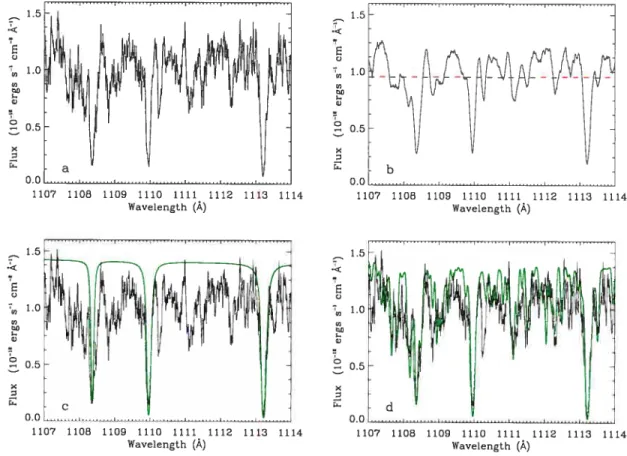
file form, regrouped by individual exposure and by channel. The last step is to co-add the
individual exposures after cross-correlating them. The correction associated with wavelength shifts was carried out by using photospheric lines. Figure 2.1 shows the spectra of the five PC 1716+426 stars analyzed here, while Figure 2.2 displays the five comparison stars using the same format. Note that the spectrum of the program object PG 1338+481 does flot include the LiF2A segment. This has forced us to work with the LiF1B channel (plotted in Figure
2.1) only, a channel that includes a notable flux drop around 1150
À,
the “worm”, which originates in an obstruction caused by grid wires placed 6 mm above the microchannels plate detector. Up to 40 % of the light can be lost through this defect.2.4
Synthetic Spectra
2.4.1
Atmospheric Parameters
The atmospheric parameters of the long-period sdB pulsators were taken from the ongoing large-scale investigation of Green et al. (2006). A progress report can be found in Fontaine et al. (20065). These parameters are based on medium-resolution optical spectra secured since
1996 at the Multiple Mirror Telescope using the MMT blue spectrograph. The spectra are
then analyzed in a homogeneous manner with the standard une fitting method (Bergeron et al.
1992). For the hydrogen-ricli subdwarfs, both the Balmer unes and the Me I transitions are fit with line-blanketed LTE and NLTE model atmospheres that include hydrogen and helium.
Line blanketing by heavy elements in the mode! atmosphere analysis is omitted since the abundances of heavy elements are not fixed a priori and are known to vary from one sdB to
another. Because our analysis is, in great part, a comparative one between two sets of objects (the PC 1716+426 stars vs. the constant and V361 Hya variables) analyzed in a consistent manner, we take advantage the homogeneity afforded by the Green et al. (2006) investigation. The atmospheric parameters we adopt for the set of five PG 1716+426 stars are given in Table
2.2, while those that characterize our reference sample are given in Table 2.3. Note that we
provide estimates of the atmospheric parameters for both NLTE fits (llpper line) and LTE fits (lower line) in these tables. Typical internal errors in the fits are of the order of ±300 K in
Teif and ±0.03 in log g. These lead to uncertainties in the derived abundances of generally less
than 0.1 dex. Systematic errors associated with the continuum setting procedure and with the particular choice of model atmospheres used in the analysis of Green et al. (2006) are undoubtedly larger, however (see below).
Two PG 1716+426 stars, the prototype and PG 1627+017, had previously been observed by Morales-Rueda et al. (2003) with the Intermediate Dispersion Spectrograph at the 2.5-m Isaac Newton Telescope at a resolution co2.5-mparable to that of the MMT data, and their parameters are included in Table 2.2. The differences in the derived atmospheric parameters
between the two analyses assuredly refiect the different assumptions used in the construction of the models. While Morales-Rueda et al. (2003) use LTE models with solar abundances of
heavy elements, the grids used by Green et al. (2006) make use of both LTE and NLTE models with a composition of hydrogen and helium only (see also For et al. 2006). It is interesting to point out that the H/He NLTE parameters are found between the LTE values based on models with solar abundances and those based on models with no heavy elements. We adopt the NLTE parameters in our analysis.
For the parameters (Table 2.3) of the comparison stars, we list the Green et al. (2006) values if the star is part of the MMT sample (this is the case for HD 4539, Feige 4$ and PG 1710+490), as well as those determined in other recent studies. Despite varions differences in the level of sophistication of the models atmosphere calculations used, no significant disparity
is observed between the Green et al. (2006) resuits and those from other investigations, at
least for the objects belonging to our reference sample.
2.4.2
Model Atmospheres and Synthetic Spectra
After securing the atmospheric parameters, we use
a
slightly updated version 200 of TLUSTY (Hubeny & Lanz 1995), as well as SYNSPEC version 4$ (Lanz 2004), to gene rate model atmospheres and synthetic spectra. Ail models are caiculated within the LTE assumption, with hydrogen and helium as the only opacity sources. In the synthetic spectra, the contribution of the heavy elements to the opacity is fully accounted for. The choice of LTE instead of NLTE models is justified for reasons of simplicity and by the fact that this investi gation is first and foremost a comparative study of the abundance pattern in two subgroups of cool sdB stars.2.4.3
Defining the Ultraviolet Continuum
Work on sdB stars in the far-ultraviolet (FUV) range presents a particular challenge, as this region is generally very crowded (e.g., Ohi et ai. 2000). This makes the placement of the continuum a particularly hazardous procedure, as a large fraction of the “noise” seen in FUSE spectra may be attributed to unresolved blends (e.g., Pereira et al. 2006). This, in turn, may contribute to increasing the systematic error on the abundance of heavy elements as compared to other determinations not affected by this crowding, as is the case in the optical or in the
near-ultraviolet (NUV), for example (see, e.g., the comparison in the case of PC 1219+534 in F igure 3 of O’Toole & Heber 2006).
The problem of setting the continuum is particularly relevant here because our analysis is of a comparative nature, in that it attempts to highlight the differences (or absence thereof) in chemical abundances between two subgroups of objects. furthermore, the hydrogen-rich subdwarfs do not form a homogeneous class with respect to abundances, and disparities in the richness of the une spectrum in the FUSE range are not uncommon. In addition, for a given object, the line density and flux level can also vary signiflcantly accross the spectrum. For ail these reasons, a consistent and robust procedure of definition of the continuum appears essential.
Two procedures have recently been discussed to try to circumvent the problems posed by the setting of the continuum. Both make use of information available outside of the FUSE range. Deetjen (2000) combines FUV data in the 912-2000
À
range from ORf EUS II echelle observations and NUV data in the 2000-3400À
range from the TUE archives. The normali zation of the reddened synthetic fluxes is then based on the range just above 3000À,
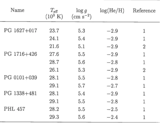
and thus altogether avoids the region crowded with unes of heavy elements in the FUV part. A different procedure was used by Pereira et al. (2006), who derive atmospheric parameters in the visible part of the spectrum, and subsequently normalize their theoretical fluxes at the y magnitude. In both cases, the normalized model spectrum defines a local continuum close to the upper envelope of the numerous hues, higher than it would be set were the structure of the ultraviolet fluxes interpreted as “noise”.The procedure we have devised in the present investigation relies exclusively on information within the FUSE range. We define flrst a region 10
À
to 20À
wide within which the continuum level has to be determined and smooth the spectrum in that region. We then define a threshold typically two-thirds of the maximum flux level within the region —below which data pointswill be subsequently ignored. The remaining fluxes are then averaged, and the continuum level
is set by multiplying the average by a flxed factor,
f.
Numerous experiments with variousobjects and spectral regions show that a value of
f
1.20 provides a reasonably satisfactory2.3 in the case of the silicon abundance in PG 1716+426.
2.5
Method of Analysis
2.5.1
Technique of Analysis
The abundances are based on
a
x2
minimization technique which relies on the continuum setting procedure described in the preceding section. Individual regions, typicaiiy 10-20À
wide, are chosen so that the biending of the unes of interest with unresoived transitions is minimized. We use the Kurucz une lists (Kurucz & Beli 1995) to construct our synthetic spectra. Within each region, we first apply a wavelength shift to bring the observed spectrum in une with the iaboratory one. The abundances of individuai elements are then determined one at a time, a procedure that permits an immediate visualization of the effect of the element on the continuum. The internai consistency of the abundances determined is improved when two channeis cover the same wavelength region. When small discrepancies arise between the abundances determined from different unes associated with a given ionization state, we favor
- quite reasonably - the strong unblended transitions located in spectral regions characterized
by good S/N ratio. Overall, given the homogeneity of the objects analyzed, we did end up anaiyzing the same limes from one star to the next. We list in Tabie 2.4 and Tabie 2.5 the principal unes used in this analysis. These hsts are simiiar to those used by Fontaine et ai. (2006a).
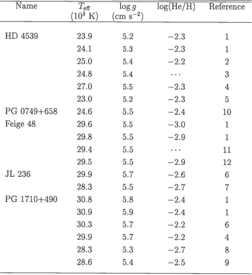
A typical resuit of the spectral synthesis achievable in PC 1716+426 stars with the element
abundances we determine is shown in Figure 2.4. It features the 1062-1074
À
region in PG 1338+481.2.5.2
Microturbulent and Rotational Broadening
Severai studies suggest that microturbuient broadening is not important in hot B subd warfs, with inferred velocities generally below 2 kms(see, most recently, Edelmann 2003;
O’Toole & Heber 2006). On that basis, we have opted flot to inciude this broadening me chanism in our synthetic spectra. In contrast, the role of rotationai broadening in the fitting
of unes of heavy elements in hot B subdwarfs might 5e more important, given that four of our five PG 1716+426 stars are in close binary systems, paired with a white dwarf: PG 1627+017 (20 hr-period; For et al. 2006; Morales-Rueda et al. 2003); PG 1716+426 (43 hr period; Morales-Rueda et al. 2003); PG 0101+039 (14 hr-period; Moran et al. 1999); and PHL 457 (<2.4 day-period; Edelmann et al. 2006b). Hot B subdwarfs in binary systems can be characterized by measurable rotational velocities, and even 5e tidally locked (Napiwotzki et al. 2001) if they are close enough, as the rapidly rotating (ysini 97±9 kms’) star KPD 1930-2752 (Geier et al. 2006) attests. Since the majority of sdB binaries have significantly longer periods, perhaps a more typical situation would 5e those of PG 1627+017 and Feige 48, for which the assumption of tidallocking suggests a rotational velocity of 15.Skms’ and of26.9kms’, respectively(For et al. 2006; O’Toole et al. 2004a). Because of this, it may be necessary to include rotational broadening in our synthetic spectra when it is deemed that additional broadening is required to match the observed hues.
This is the case, for example, for PHL 457, one of our target stars. Our preliminary fits suggest that a projected rotational velocity of the order of 20 km s1 is required to match the line widths. The inclusion of a velocity of this order improves the overall quality of the fit, but changes the abundances by only 0.2 dex compared to our fits without rotation. For the other stars, projected rotational velocities of the order of 5 — 10 kms1 lead to small improvements in the quality of the fits, and could very well have been included in our analysis. This being said, it is clear that the determination of rotational velocities in hot B subdwarfs (see, e.g., Edelmann et al. 2006a) deserves to 5e examined as a separate issue and we will return to this topic in a separate paper. For the present investigation, we simply list, in Table 6, the abundance values secured with no rotation velocity. The same situation prevails in the case of the reference stars; there, however, we must point out that the quality of our fits to Feige 48, our reference V361 Hya star and a short-period binary sdB (O’Toole et al. 2004a), is also improved by including a small additional broadening, amounting to vsini ‘ 2Okms’. We
are aware that, for this object, Heber et al. (2000) and O’Toole & Heber (2006) constrain the projected rotational velocity to vsini < Skms’, on the basis of the narrow hues observed in the optical and in STIS spectra in the 1160-2300
Â
range. For pulsating stars, it is possiblethat the surface motions associated with the pulsations, rather than rotation, might contribute to the observed une broadening, as suggested by Kuassivi et al. (2005) for the large-amplitude
(‘-- 0.25 mag) V361 Hya variable PG 1605+072.
2.5.3 Sources of Error
Three types of errors affect our abundance determinations: those associated with the deter minations by Green et al. (2006) ofthe atmospheric parameters (Teff, log g, and log N(He)/N(H)), those associated with our fitting technique (setting of the continuum, handling of blends, etc), and finally those associated with the input physics used in the calculation of the model at mospheres and synthetic spectra.
The first of these has already been discussed in
§
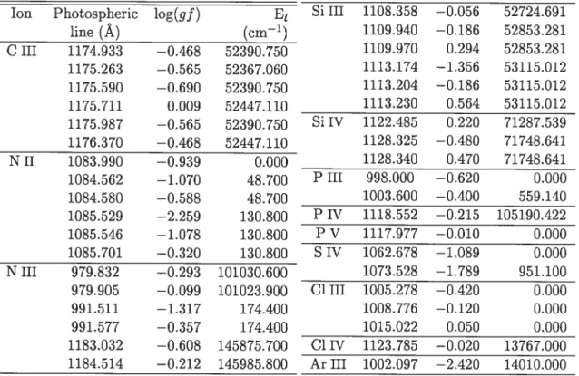
2.4. There, an uncertainty of less than 0.1 dex has been assigned to the determination of the atmospheric parameters within the Green et al. (2006) model grid. The uncertainty is likely to be somewhat larger if one includes the systematic effects associated with the inclusion or omission of lime blanketing by heavy elements in the model atmosphere. We note, in this respect, that the Morales-Rueda et al. (2003) models make use of solar abundances of heavy elements, abundances that overestimate by a considerable margin those determined here. For this component, then, we adopt a 0.2 dex uncertainty.A further error comes from the part of the analysis which deals specifically with the pla cement of the continuum. We show, in Figure 2.5, the performance of our technique on a synthetic spectrum to which we have added an increasingly larger noise level so as to simu late a FUSE spectrum. The nominal abundances included in the calculation of the synthetic spectrum are solar, except for iron for which we use log N(Fe)/N(H) = —4.2. Our continuum
setting technique in the 1116—1133
Â
region permits us to recover the input iron abundance to within 0.2 dex for $/N ratios as low as 5, and within 0.3 dex for a S/N ratio of 3.All in ail, thus, we estimate the uncertainty linked with the setting of the continuum to be of the order of 0.2 — 0.3 dex on the basis of the numerous experiments we carried out in our attempts to devise a robust and consistent method to define the continuum in our spectra. It is clear, however, that the continuum setting procedure remains the Achilles heel of any
abundance analysis that must rely on weak unes (like those of the iron-peak elements) in heavily blanketed spectra (like the FUSE spectra of sdB stars). While the comparison of the preliminary abundances of Blanchette et al. (2006) with the final values given here provides a sobering reminder of this state of affair, we believe that our continuum setting procedure now provides us with a robust and consistent way to define the continuum in the FUSE spectra of PG 1716+426 stars.
With the continuum defined by a consistent and robust method, additional uncertainties arise from the
x2
technique itself. Depending on the intensity and the S/N ratio of the lines observed, the weight associated with the core or the wings of the unes can give rise to an additional ±0.1 dex uncertainty. Blends arising from ISM lines or from unidentified photo spheric transitions may also be present, but can generally be avoided by choosing to emphasize spectral windows relatively free from contamination. We note that the use of alternative ways to set the continuum, and even of spectral regions beyond the FUSE range, may lead to dif ferent abundances, but will affect to a less extent those conclusions which rely on a relative determination of abundances in two distinct samples.The third component to the errors is associated witli the physics included in our models. Microturbulent broadening is consistently small in these objects, but a maximum uncertainty of ±0.2 dex is stiil associated with the additional broadening required in the specific case of PHL 457. Additional uncertainties are associated with possible NLTE effects in the hue transfer(which may show up in the abundances we determine being sensitive to the particular ionization state chosen) and with the atomic data used in SYNSPEC (especially the log gf values) which become more uncertain as the excitation energy of the levels increase. For this component, thus, we adopt a 0.3 dex uncertainty, while keeping in mmd that this estimate
is perhaps too generous for those objects which show hittle trace of additional broadening.
Overall, thus, we find that a combined uncertainty of the order of ±0.4 — 0.5 dex appears
2.6
Determination of Element Abundances
2.6.1
The Light flements
Let us first compare the abundances of light elements amongst the PG 1716+426 stars. They are summarized in Table 2.6 and in Figure
2.6.
From carbon to argon, all five PG 1716+426 stars exhibit similar trends, and these resuits are generally in line with those from past investigations (see, e.g., Lamontagne et al. 1985; Heber et al. 2000; Ohl et al. 2000; Edelmann 2003; Edelmann et al. 2003; O’Toole & Heber 2006): abundances close to the solar value for N; slight underabundances for S, perhaps not as marked as those found by Edelmann (2003); underabundances for the elements C, Si, P, and Cl. For Ar, we can only provide upper limits. since our determination is based on a single line which appears blended with a H2 une from the 15M. This is especially evident in PG 1627+017 where the 15M contamination involves a strong saturated line riglit on top of the Ar line. We consequently refrain from estimating the Ar abundance in that object. Most of the limits — save that assigned to PG 0101+039 suggest an Ar deficiency. This contrasts with the result of Edelmann (2003), who generally finds Ar enrichment in his sample.Our sample of comparison stars was analyzed in a similar way. Because the objects it contains cover roughly the same range in effective temperature as the PG 1716+426 stars, there are no theoretical reasons to expect differences between the average abundances of light elements in the two samples and this is indeed what we find. In particular, the FUSE-based pper limits are consistent with an Ar abundance at or below the solas value whule, for example, Edelmann (2003) find Ar enrichment by a factor 3 in the normal sdB stars Feige 65 (Teff 23, 900 K) and Feige 36 (Teff = 29,700K).
2.6.2
Iron-Peak Elements
Because the driving of the non-radial pulsations observed in the PG 1716+426 (as well as in the V361 Hya) stars is thought to be intimately related to the presence of a levitating reservoir of iron-peak elements in the envelope of these stars, the observation of strong abundance anomalies in the PG 1716+426 stars as a whole, as well as that of systematic differences
between the abundances in PG 1716+426 stars and in constant stars, might yield interesting constraints on current non-adiabatic models. This has been the hope and motivating force behind this investigation. However, as indicated above, it may also be the case that the atmospheric abundances have littie to reveal about the abundances of the iron-peak elements in the driving region because of the blurring effects of diffusion. Let us discuss then our main resuits.
We find here that the long-period variables are characterized, as a group, by very homo geneous abundances of the iron-peak elements V, Cr, Mn, Fe, Co, and Ni, which all tend to 5e in their doubly-ionized state. For V, for which upper limits only are available, the average value of this limit is a factor 15 above the solar value (logN(V)/N(H) = —8.0) and littie
can be said about a potential abundance anomaly for that element. For Cr, Mn, Fe, and Co the average abundances determined in the sample are, respectively, logN(Cr)/N(H) = —6.0;
logN(Mn)/N(H) = —6.2; logN(Fe)/N(H) = —4.2; logN(Co)/N(H) = —6.4. These abun
dances are, respectively, +0.4, +0.4, +0.4, and +0.7 dex above the solar value. In other words, an average overabundance is noted with respect to the solar value, by factors ranging from 2.5 for Cr, Mu, and Fe to 5 for Co. The abundance of Ni appears less homogeneous: four stars, PG 1716+426, PG 0101+039, PG 1338+481, and PHL 457, display significant underabundances with respect to the solar value, by —1.7 dex on the average, while the fifth object, the cool star PG 1627+017, exhibits a significant overabundance, by a factor 40, with respect to the Sun. The strongest Ni lines available, around 979.5
À,
are contaminated with iron and chromium transitions, and are also located in the wings of strong nitrogen unes. Given that O’Toole & Heber (2006) have observed generally larger Ni abundances in the NUV, it is possible that the crowding observed in the FUSE spectra might play a role in accounting for the spread we observe and for a larger systematic difference in the abundance of that element.The second interesting aspect of our investigation resides with the abundance determi nations in the reference sample. We refrain from giving a full list individual values here, as the reference sample is included in the detailed analysis of Fontaine et al. (2006a). Thus, we simply refer here to average values for this sample. Let us consider the four constant stars first. For vanadium, we again find only upper Hmits and the average value of this limit is +0.3
dex above that of the PG 1716+426 stars. For Cr, Mu, and Fe the average abundances in the constant stars differ by, respectïvely, —0.1, 0.0, and —0.2 from their counterparts in the PG 1716+426 stars. For cobalt, only upper limits are available in the constant stars, and the average value of these limits is +0.6 dex above the average abundance determined in the PG 1716+426 stars. For nickel, we secured measurements for only two of the four constant stars and the average is +1.0 dex above the average abundance in the PG 1716+426 stars. For the other two stars (HD 4539 and PG 0749+658, both plagued by inferior data), the upper limits secured are +2.5 dex above the average abundance determined in the long-period variables. The overail impression, thus, is that the constant stars do not exhibit abundances of iron-peak elements that differ significantly from those measured in the PC 1716+426 stars. In the few cases where one has to compose with upper limits (Co, Ni), the abundances in the constant stars could equally well 5e higher or lower than in the PC 1716+426 stars. Only in the case of V is the possibility excluded that the average abundance in the constant stars be larger than that in the PG 1716+426 stars. In the case of our loue V361 Hya pulsator, Feige 48, the Cr, Mu, and Fe abundances are within 0.3 dex not only from the average abundance of the same element in the PC 1716+426 stars but also from the average abundances determined in the constant stars. The end resuit is that there does not appear to be essential differences in the atmospheric abundances of the iron-peak elements between pulsators and non-pulsators alike. We are thus unable to identify a spectroscopic signature which would allow a distinction between those two types of stars to be made.
According to the thinking of Fontaine et al. (2006b), in a constant cool B subdwarf, Fe could 5e overabundant or underabundant with respect to, or even at, the solar value, while a pulsator is likely to be characterized by an enhanced value of the abundance of that element. Quantitatively, their discussion suggests that the driving of pulsations will be favored for surface iron abundances roughly above 1.5-10 times the solar value. If we were to take these numbers at face value, then we could argue that the overabundance factor appears only marginally consistent with the theoretical requirements expressed by Fontaine et al. (2006b) given that only a slight overabundance of iron-peak elements is observed in the FUSE spectra. However, the theoretical expectations are quite specific to the one model they investigated,
i.e., one with M =0.5 M®, 10g 9 5.5, T 30,000 K, with a wind mass loss rate of 6 x
M0 yr’. A detailed exploration of the parameter space seems clearly warranted, but lias yet to be performed. At this stage, thus, we can only conclude that, whule the present analysis does not provide strong support for the views expressed by Fontaine et al. (2006b), it is flot inconsistent with such a scenario. In particular, the wind model discussed by Fontaine et al. (2006b) does imply the presence of iron-peak elements at detectable levels in the atmospheres of pulsating sdB stars. This is what was found here.
From a broader perspective, the interplay between the abundance of iron-peak elements, the location of the reservoir, the age of the star, and the mass-loss rate appears so complex (Chayer et al. 2004; Fontaine et al. 2006b) that it may unfortunately not be possible to distinguish, in the end, constant stars from PG 1716+426 or V361 Hya variables on the sole basis of their atmosphericabundances of iron-peak elements.
2.6.3
Elements Beyond the Iron Group
Given the recent discovery of elements beyond the iron peak in both white dwarfs (Vennes et al. 2005; Chayer et al. 2005) and hydrogen-rich hot subdwarfs (O’Toole 2004; O’Toole & Heber 2006; Chayer et al. 2006), we have searched for these elements in our sample of PC 1716+426 stars. In general, the abundance of the heavy elements germanium, zirconium, tin and lead are fixed by a few lines only, sometimes even by a single line, and blending with Fe, Cr, and Mn is also possible. This is the case, for example, for Zr IV and Sn II which require special care.
Let us consider first the case of Zr IV. To be able to use the resonance transition at 1183.937
À,
Chayer et al. (2006) had to estimate its oscillator strength by matching the Zr abundance derived for Feige 48 both from FUSE and from longer-wavelength STIS data (specifically, the 1790.113À
and 1793.523À
transitions). We use the gf value determined by Chayer et al.(2006) here as well. In addition, we have modified SYNSPEC 48 to generate synthetic spectra
associated witli elements of atomic number larger than 28 and with ionization stages 3. For
Zr IV, the partition function is simply estimated from its first term, U 2j + 1 = 4. Because
elements. For Sn II, the strongest unes available, albeit flot that strong, are ail blended with other transitions and can only be used to set upper limits on the abundance.
The cases of Ce III and Ph III are more conventional, as the unes involved are a priori
isolated. The fundamental transition at 108$
À
for Ce III and the one at 1048.877À
for Pb III yield, for the majority of objects, a good indication of the abundance, even thongh we are dealing, in each case, with a single une from one ion. The abundances of these elements in the sample of PC 1716+426 stars are also summarized in Table 2.6 and in Figure 2.6. They follow the general trends already found by O’Toole Si Heber (2006) and Chayer et al. (2006), namely a strong overabundance of these very heavy elements in the photospheres of snbdwarf B stars.2.7
Summary and Conclusion
In this paper, we compared the photospheric abnndances in bye long-period pulsating sdB stars with those encountered in a sample of reference objects that includes one short-period V361 Hya star and four constant stars. The aim xvas to test the ideas that long-period variables and constant stars might be distinguishable on the basis of photospheric abundances, and that a weak stellar wind could play a central role in the evolution of the pulsations of sdB stars, through the depletion of the reservoir of iron-peak elements responsible for the driving of the pulsations. Special care was taken to ensure the homogeneity of the analysis, both in the source of data used and in the technique of analysis. This is particularly important in this case, as abundance determinations of heavy elements in hot B subdwarfs still display small systematic differences which may result from the different data sets (STIS vs. FUSE) and analysis techniques (e.g., the continuum setting procedure, which appears easier in STIS data than in FUSE data) used.
We find no significant differences in the abundances of the important iron-peak elements between the long-period variables and the reference sample. This is in une with the prelimi nary results of O’Toole et al. (2004b) and O’Toole Si Heber (2006), who investigated V361 Hya stars only. In addition, the observed enhancements of iron-peak elements found in the PC 1716+426 stars are quite modest, except perhaps for Co where the overabundance appears
more spectadular. With a proper allowance for systematic errors, our resuits are not incon sistent with the general picture outlined by Fontaine et al. (2006b) on the basis of a calculation that follows in some detail the emptying of the iron reservoir through wind mass-loss. The calculations follow the abundance of iron during i08 yrs, the typical lifetime on the EHB. The prediction, made on the basis of a single mass loss rate of 1i1 = 6 x i0 M® yr1 and for
typical values of M = 0.5 MG, log g 5.5, = 30,000 K, is that pulsators should show some
photospheric Fe enhancement by factors of at least 3 to 4, while constant stars could be cha racterized by depleted, normal, or enhanced abundances. While formally consistent with these very general expectations, our results do not provide overwhelming support for this picture either. Given the expected sensitivity of the predicted envelope abundances to atmospheric parameters, wind mass loss rate and stellar age, much work remains to be done before this issue gets resolved. In the end, it could very well be the case that what we aimed for, that is a spectroscopic signature that would discriminate between pulsators and non-pulsators, simply does not exist, and that the observed atmospheric abundances may reveal very little sign of the expected overabundances of iron-peak elements deep in the driving region.
2.8
Acknowledgements
This work was supported in part by the NSERC of Canada and by the FUSE Project funded by NASA contract NAS5-32985. G.F. also acknowledges the contribution of the Canada Research Chair Program.
2.9
Tables
TABLEAu 2.1 — Summary of the FUSE observations
Target
VProgram ID
Data acquisition
Number of
Exposures
Data set
mode
exposures
time (sec)
PG 1627+017 12.93a E1220901 TTAG 2 2549
PG 1716+426
13.gZa
B0541301
TTAG
5
6074
PG 0101+039
12.06
E1220101
HI$T
4
1486
PC 1338+481
13.64e’
E1220501
TTAG
7 14106PHL 457
12.95
E1221201
TTAG
9
10143
TABLEAu 2.2 — Atmospheric parameters of pulsating sdB stars
Name I logg log(He/H) Reference
(i0 K) (cm e_2) PG 1627+017 23.7 5.3 —2.9 1 24.1 5.4 —2.9 1 21.6 5.1 —2.9 2 PG 1716+426 27.6 5.5 —2.9 1 28.7 5.6 —2.8 1 26.1 5.3 —2.9 2 PG 0101+039 28.1 5.5 —2.8 1 29.1 5.7 —2.7 1 PC 1338+481 28.1 5.4 —2.9 1 29.1 5.5 —2.8 1 PHL 457 28.2 5.5 —2.5 1 29.3 5.6 —2.4 1
TABLEAU 2.3 — Atmospheric parameters of comparison sdB stars
Name Tff logg log(He/H) Reference
(l0 K) (cm
s2)
HD 4539 23.9 5.2 —2.3 1 24.1 5.3 —2.3 1 25.0 5.4 —2.2 2 24.8 5.4 ... 3 27.0 5.5 —2.3 4 23.0 5.2 —2.3 5 PG 0749+658 24.6 5.5 —2.4 10 Feige 48 29.6 5.5 —3.0 1 29.8 5.5 —2.9 1 29.4 5.5 ... 11 29.5 5.5 —2.9 12 JL 236 29.9 5.7 —2.6 6 28.3 5.5 —2.7 7 PG 1710+490 30.8 5.8 —2.4 1 30.9 5.9 —2.4 1 30.3 5.7 —2.2 6 29.9 5.7 —2.2 4 28.3 5.3 —2.7 8 28.6 5.4 —2.5 9References. (1) Green et al. (2006) NLTE top une, LTE bottom une; (2) Baschek et al. (1972); (3) Heber & Langhans (1986); (4) Saffer et al. (1994); (5) Edelmann (2003); (6) Fontaine et al. (2006a); (7) Heber (1986); (8) Moehler et al. (1990); (9) Theissen et al. (1995); (10) Ohl & Chayer (2006); (11) Chayer et al. (2003); (12) Heber et al. (2000);
Ion Photospheric log(gf) E1 Si 111 1108.358 —0.056 52724.691 une
(À)
(cm—’) 1109.940 —0.186 52853.281 C III 1174.933 —0.468 52390.750 1109.970 0.294 52853.281 1175.263 —0.565 52367.060 1113.174 —1.356 53115.012 1175.590 —0.690 52390.750 1113.204 —0.186 53115.012 1175.711 0.009 52447.110 1113.230 0.564 53115.012 1175.987 —0.565 52390.750 Si IV 1122.485 0.220 71287.539 1176.370 —0.46$ 52447.110 1128.325 —0.480 71748.641 N II 1083.990 —0.939 0.000 1128.340 0.470 71748.641 1084.562 —1.070 48.700 P III 998.000 —0.620 0.000 1084.580 —0.588 48.700 1003.600 —0.400 559.140 1085.529 —2.259 130.800 P IV 1118.552 —0.215 105190.422 1085.546 —1.078 130.800 P V 1117.977 —0.010 0.000 1085.701 —0.320 130.800 5 IV 1062.67$ —1.089 0.000 N III 979.832 —0.293 101030.600 1073.528 —1.789 951.100 979.905 —0.099 101023.900 Cl III 1005.278 —0.420 0.000 991.511 —1.317 174.400 1008.776 —0.120 0.000 991.577 —0.357 174.400 1015.022 0.050 0.000 1183.032 —0.608 145875.700 Cl IV 1123.785 —0.020 13767.000 1184.514 —0.212 145985.800 Ar III 1002.097 —2.420 14010.000TABLEAU 2.4 — List of the photospheric unes not belonging to elements of the iron peak
(see next table) that were used to determine the atmospheric composition of the sdB
TABLEAU 2.5 — Similar to table 2.4, but for iron-peak elements and beyond. Here again, Ion log(gf) VIII Cr III FellI 1061.244 —0.945 30725.801 1061.818 —1.445 30725.801 Photospheric Et 1062.272 —1.412 30716.199 une


![TABLEAU 2.6 — Observed abundances (log[(N(X)/N(H)]), as determined from indicated](https://thumb-eu.123doks.com/thumbv2/123doknet/7229174.202972/43.918.168.791.392.917/tableau-observed-abundances-log-n-x-determined-indicated.webp)