Science Arts & Métiers (SAM)
is an open access repository that collects the work of Arts et Métiers Institute of
Technology researchers and makes it freely available over the web where possible.
This is an author-deposited version published in: https://sam.ensam.eu Handle ID: .http://hdl.handle.net/10985/14158
To cite this version :
Sylvie LHOSPITALIER, Philippe BOURGES, Alexandre BERT, Jean QUESADA, Michel LAMBERTIN Temperature measurement inside and near the weld pool during laser welding -Journal of Laser Applications - Vol. 11, n°1, p.32-37 - 1999
Any correspondence concerning this service should be sent to the repository Administrator : [email protected]
Temperature measurement inside and near the weld pool
during laser welding
S. Lhospitalier
LABOMAP–ENSAM, Ecole Nationale Supe´rieure d’Arts et Me´tiers, Laboratoire Bourguignon des Mate´riaux et Proce´de´s, 71250 Cluny, France
P. Bourges
CLI Ceusot Loire Industrie, Centre de Recherche des Mate´riaux du Creusot, France A. Bert, J. Quesada, and M. Lambertin
LABOMAP–ENSAM, Ecole Nationale Supe´rieure d’Arts et Me´tiers, Laboratoire Bourguignon des Mate´riaux et Proce´de´s, 71250 Cluny, France
~Received 2 May 1998; accepted for publication 6 November 1998!
The work in this article deals with the measurement of temperature fields inside and near the weld pool during laser welding. The laser source used for this study is a 7.5 kW CO2laser, and the welded
material is a UNS N08904 austenitic stainless steel. The principle behind the actual experimentation is relatively simple: the welding operation is recorded with a charge coupled device camera equipped with infrared filters; after calibrating the camera sensor and image processing, the temperature distribution in the weld pool and near the melted zone is revealed. © 1999 Laser Institute of America.@S1042-346X~99!00401-5#
Key words: CO2laser welding, temperature measurement, austenitic stainless steel
I. INTRODUCTION
To better understand thermomechanical phenomena that occur during laser welding, it is necessary to know the tem-peratures inside the weld pool and near it. Many numerical simulations can be found in the literature,1–3but little experi-mental data concerning thermal cycles inside the weld pool are available. The great difficulty of such experiments is the very high temperatures that are reached by the treated mate-rial, especially steels. In this article, we describe the experi-mental method used to determine the thermal field around laser impact during welding of austenitic stainless steel. The study is conducted on 8 mm thick sheets. Two characteriza-tion methods have been used. The temperature inside the material is determined with thermocouples, and that on its surface is determined by use of a charge coupled device
~CCD! camera equipped with infrared ~IR! filters. The results
obtained by these two methods may be used as a database for numerical simulation.
II. PRESENTATION OF THE EXPERIMENTAL PARAMETERS
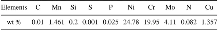
The material used is austenitic stainless steel UNS N08904~CLI URB6™!, which contains low phosphorus and sulfur levels. The actual composition is given in Table I.
The sample size was chosen so that the temperature at the border remains approximately constant ~i.e., room tem-perature!. To control this, eight thermocouples were placed along the sample, and the border temperatures during weld-ing were recorded. These measurements gave us a sample size of 215 mm380 mm. Moreover, to reproduce the me-chanical behavior of a massive piece, the samples were bridled on a steel block with six screws. Finally, to avoid gap
problems between the two sheets, fusion lines ~keyhole welds! were realized, instead of real welding of the two sepa-rate sheets~Fig. 1!.
III. THERMAL MEASUREMENTS WITH THERMOCOUPLES
The temperatures measured ranged between 1000 and 1800 °C ~the melting temperature of UNS N08904 is 1380 °C!. That is why tungsten ~W5 type! thermocouples were used. They have a good resistance to high temperatures, and their small diameter~0.2 mm! results in a small tempera-ture lag time. The diameter of the entire thermocouple was 1.2 mm ~including the tungsten wires and sleeving!. The thermocouples were placed inside the samples, 4 mm under the surface, into 1.4 mm diam holes made by electroerosion, inclined 20° from horizontal to disturb the thermal fields as little as possible~Fig. 2!. Eight samples were machined, then two thermal cycles were characterized ~four measurements for each thermal cycle!. Because thermal cycles are very short during laser welding, it was necessary to choose a suf-ficiently high acquisition rate. The maximum rate authorized by the system used is 100 measurements per second provid-ing that there is only one thermocouple at a time workprovid-ing. Then, we had to put one thermocouple per sample in place and perform as many weldings as necessary.
TABLE I. Composition of the stainless steel used.
Elements C Mn Si S P Ni Cr Mo N Cu
The process parameters chosen for the two thermal cycles were very close: 5 kW, 0.5 m/min and 6 kW, 0.5 m/min. The results obtained are similar for these two cycles, that is why we shall present just the latter one. The widths of the melted zones are approximatively 7 mm on the surface of the sheet and 2 mm inside the material ~Fig. 3!.
The curves in Fig. 4 show the evolution of the thermal gradients inside the samples with time. Time 0 indicates that the laser beam is situated on a given point ~the temperature maximum in the center of the weld!, and abscissa 0 repre-sents the center of the weld ~the X axis being perpendicular to the joint!.
Upon arrival of the laser beam, there is a sudden rise in temperature in the center of the weld, whereas the rest of the sample remains cold. Very quickly, heat is transmitted by conduction to the rest of the sheet. The result is that the zones most distant from the center of the weld start to heat up while the nearest zones start to cool down. This is shown by the progressive slope of the curves. At the end, these curves become parallel, and the entire sample cools down. This phenomenon, so called differential heating, is very im-portant in explaining deformations during welding.4
Figure 5 gives a different concept of heating differences according to the distance of the point measured from the center of the weld. For instance, points which are 2 mm from the center of the weld receive maximum thermal flux 5 s after the beginning of the recording.
IV. SURFACE TEMPERATURE MEASUREMENTS WITH AN IR-CCD CAMERA
In order to complete these observations, we have mea-sured surface temperatures using a CCD camera equipped with infrared filters. Two additional cycles were completed: 5 kW, 0.4 m/min and 6 kW, 0.5 m/min.
Infrared imagery consists of recording an image of light intensity emitted by a fixed wavelength target in the infrared domain. Usually this method is conducted with thermal cam-eras equipped with light intensity sensors sensitive to wave-lengths that are often far ~several microns! from the visible. The construction of infrared cameras is complex, and special materials are needed for optical sensors, an optomechanical scanning system~used to read images!, temperature balance of the equalization system~used to avoid measure drift due to camera heating!, rigorous calibration etc.5,6This method is not very easy to use.
To perform our experiments, a classical CCD camera was transformed into a pseudothermal camera. The CCD sensor of the camera has to be sensitive to infrared radiation
~usually the nearest infrared!. This related technique permits
an initial approach to temperatures inside the weld pool and near it with sufficient accuracy for our purpose.
The camera chosen has good features in the infrared do-main~seen in Fig. 6!. CCD classical cameras are sold with a ‘‘cold filter,’’ which ‘‘cuts’’ the infrared radiation for com-mon application or use. In our case, it is necessary to take
FIG. 1. Geometry of the samples.
FIG. 2. Thermocouple locations: ~a!585 mm61 mm ~always the same!; (b)540, 39, 38, 37 mm60.1 mm @~b! takes four different values for each thermal cycle#; ~c!54 mm60.1 mm.
FIG. 3. Geometry of the welded joints.
this away. The interaction between the laser beam and the treated material gives high intensity radiation because of the melted pool and the surface plasma. It is necessary to do a filtration of the major part of this radiation. It is known that plasma radiation takes place preferentially in low wave-lengths and in the ultraviolet zone.7 So it is interesting to observe the weld pool in the infrared domain since the re-sidual plasma radiation will be lower. However, the experi-mentation wavelength bandwidth is limited by the camera sensor technology. Figure 6 shows that total infrared radia-tion is cut at 1200 nm. The working wavelength is chosen as 1100 nm. To avoid the camera sensor from being saturated with light, and in order to be able to consider the material as a graybody, the wavelength bandwidth must be very narrow. The previous conditions imposed the use of an interferential filter, 1100 nm centered and 10 nm width. It is a standard filter that is a good compromise between cost and technical needs. And it is useful to indicate a problem due to the filter. Because of the technical properties of the filter, on the re-corded images we can observe interference rings, which exist for a large range of optical adjustments. The result is that the image obtained is an overlap of the original image and the interference rings~see Fig. 7!. In order to solve this optical problem, it is necessary to increase the size of the lens
aper-ture of the camera, bring the camera as close as possible from the measured point, and increase the wavelength band-width of the filter used.
In practice, none of these solutions was applicable to the experiment because of the space required on the laser ma-chine and because of an increase in the total installation cost. The remaining solution is a posttreatment computing, which will be explained later.
Analysis of infrared radiation is dependent on the emis-sivity of the material. The material’s emisemis-sivity is related to numerous parameters: direction, surface quality, physico-chemical state, temperature etc.8–10 First, it is necessary to choose a good angle of observation, taking into consideration spectral emissivity, minimization of geometrical aberrations, and the space required for the entire device. The maximum observation angle obtained was 70°. Gaseous protection is realized with helium in a glove box. Images are transmitted to the camera by two convergent standard BK7 lenses ~Fig. 8!. Braces are placed between the objective and the camera’s CCD sensor to correctly magnify the zone being observed. But, there was a big problem: vibrations of the machine tool. To eliminate them, it was necessary to put the entire optical device on an antivibrating carpet.
Images are stored using a video recorder~25 images per second!. This is a sufficient speed in this case because the welding speed is too low~0.5 m/min! as are the temperature
FIG. 5. Thermal cycles of different points inside the samples.
FIG. 6. Camera sensitivity spectrum. FIG. 7. Example of a recorded infrared image.
changes associated with it. ‘‘Key’’ images are then located precisely and digitalized before analyzing.
Before analyzing the images, it is necessary to do a cali-bration of the entire optical device, i.e., the camera 1 the interferential filter 1 the lenses associated to the test con-figuration~observation angle, distance to the sample, etc.! in order to relate the gray levels to the surface temperatures. Several methods are possible depending on the temperature range. In our case, we used direct calibration, which means that the variable emissivity and other phenomena like plasma are directly integrated. To do that, a sufficient surface area of the material is uniformally heated with a defocused laser beam; the image ~gray level! is recorded with the same op-tical device as that described previously, while the tempera-ture is measured simultaneously with a thermocouple placed just under the heated surface~Fig. 9!. A comparison of the two results ~thermocouple data and recorded images! allows one to relate the gray level recorded to a given temperature. This test is repeated for several temperatures, and it gives a calibration curve~Fig. 10!. The great advantage of this cali-bration technique is that the emissivity and other unneces-sary effects ~like plasma radiation, for example! are totally
FIG. 8. Schematic of the experimental device.
FIG. 9. Schematic of the calibration device.
FIG. 10. Calibration curve of the camera sensor.
integrated into the measurements. It is then certain that a given gray level is associated to the real temperature.
It appears that the CCD camera sensor equipped with the infrared filter was sensitive in the 1000–1800 °C temperature range. According to the shape of the curve~Fig. 10!, it ap-pears that if the gray level error is considered as being con-stant, the error in the corresponding temperature may vary, and is more important in the curve extremities. The major source of error concerning the real values of the temperature is the variation of the emissivity of the material during weld-ing ~the steel becomes brighter after solidification of the melted zone!. According to data in the literature,11the emis-sivity of rough stainless steel can be estimated as approxi-mately 0.7 and its emissivity when polished is approxiapproxi-mately 0.5. A rapid calculation using blackbody and graybody laws reveals that the error made in the temperatures is less than 8% at 3000 °C~2% at 1800 °C!. According to the experimen-tal conditions, a final maximum error of 10% can reasonably be expected.
The problem of interference rings observed during the experiments is solved by averaging the gray levels for a given temperature range. An algorithm was developed, which associates a temperature range to a gray level range according to the calibration curve. Using the algorithm, im-ages in the gray levels are automatically converted into ther-mal cards showing isotherther-mal domains. Figure 11~a! shows an example of a gray level primary image, and Fig. 11~b! shows the same image after computing the analysis.
After welding, the image of the joint was recorded, and this allows one to determine the limit of the melted zone
@Fig. 12~b!#. When compared with the temperature
distribu-tion, it can be observed that the temperature range at that limit ~1300–1405 °C! is in quite good agreement with the melting point of the steel~1380 °C!.
The maximum temperatures detected are higher than 1770 °C. A saturated zone appears~.1770 °C!, which prob-ably corresponds to the keyhole location.
One can also observe in the images weld pool asymme-try, which can easily be explained by plasma displacement due to protection gas. Moreover, for temperatures below the melting temperature, there seems to be an optical aberration: isothermal lines are distorted, which could be due to the radiation induced by laser-material interaction on the surface of the steel. But there is also another explanation of this phenomenon: as previously mentioned, the plasma is blown
by the protection gas, and this can create additional heating of the zone close to the keyhole.
V. CONCLUSION
Four different thermal cycles that occur during welding have been discussed in this study. The method which was used gives satisfactory results: good sensitivity to experi-mental parameters was exhibited. Many differences can be revealed between very close thermal cycles. For instance, the weld pool is wider for a 6 kW 0.5 m/min cycle than for a 6 kW 0.7 m/min one. So this experimental method is well adapted to characterize thermal surface phenomena inside and near the weld pool. The temperatures reached are diffi-cult to access by any other method. The most original part of this work is the camera sensor calibration, which takes the total environment~emissivity, plasma interference, operating conditions, etc.! into account. In order to do so our technique needs one calibration per material and welding configuration. A great number of images have been realized, and they will allow us to calibrate a finite element simulation of laser welding. Moreover, similar experiments will be soon con-ducted on other materials ~duplex stainless steels, for in-stance! and for other welding processes ~particularly GTAW!.
ACKNOWLEDGMENTS
The authors are very grateful to R. M’Saoubi, J. Outeiro
~LM3, ENSAM Paris!, C. Le Calvez and M. Gauthier ~CLI!
for their contribution to this work, and the Regional Council of Burgundy for its financial support.
1E. A. Metzbower, ‘‘On the temperature and size of the keyhole,’’
ICA-LEO Proceedings, 1992.
2A. Strauss and L. Pretorius, ‘‘Determination of temperature distribution in
laser welded heat exchangers with the aid of finite element method,’’ Opt. Laser Technol. 21, 381–387~1989!.
3S. Kou, ‘‘Simulation of heat flow during the welding of thin plates,’’
Metall. Trans. A 12A, 2025–2030~1981!.
4
S. Lhospitalier, ‘‘Approche thermome´canique de la fissuration a` chaud dans un acier inoxydable auste´nitique; cas du soudage laser,’’ Thesis, ENSAM, Cluny, France, 1997.
5D. Pajani, ‘‘Thermographie infrarouge,’’ Techniques de l’inge´nieur
R2740.
6
D. Pajani, ‘‘Mesure par thermographie infrarouge,’’ ADD Editeur, 1993.
7W. Sokolovsky, G. Herziger, and E. Beyer, ‘‘Spectral plasma diagnostics
in laser welding with CO2lasers,’’ Proc. SPIE 1020, 96–102~1988!.
8K. Ujihara, ‘‘Reflectivity of metal at high temperatures,’’ J. Appl. Phys. 43, 2376–2383~1972!.
9P. Herve, ‘‘Influence de l’e´tat de surface sur le rayonnement thermique
des mate´riaux solides,’’ Thesis, University of Paris VI, 1977.
10A. J. Chapman, Heat Transfer, 3rd ed.~Collier Macmillan, New York,
1974!.
11M. Huetz-Aubert, ‘‘Rayonnement thermique des mate´riaux opaques,’’
Techniques de l’inge´nieur, A1085.
This article is copyrighted as indicated in the article. Reuse of AIP content is subject to the terms at: http://scitation.aip.org/termsconditions. Downloaded to IP: 193.50.222.52 On: Wed, 05 Feb 2014 15:09:23