Passive designs and strategies for low-cost housing using simulation-based optimization and different thermal comfort criteria
Anh-Tuan Nguyen*, Sigrid Reiter
LEMA, University of Liège, Belgium
Address: LEMA, Bât. B52/3, Chemin des Chevreuils 1 - 4000 Liège
Corresponding email: natuan@ud.edu.vn; anhtuan.nguyen@alumni.ulg.ac.be
Abstract
An optimum design of low-cost housing offers low-income urban inhabitants great opportunities to obtain a shelter at an affordable price and acceptable indoor thermal conditions. In this paper, the design and operation of a low-cost dwelling were numerically optimized using a simulation-based approach. Three multi-objective cost functions including construction cost, thermal comfort performance and 50-year operating cost were applied for naturally ventilated and air-conditioned buildings. Thermal environment inside the house was controlled and assessed by two thermal comfort models. Optimization problems which consist of 18 design parameters and 6 ventilation strategies were examined by two population-based probabilistic optimization algorithms (particle swarm optimization and hybrid algorithm). Optimum designs corresponding to each objective function, differences in optimal solutions, energy saving by the adaptive comfort approach and optimization effectiveness were outlined. The optimization method used in this paper shows a considerable potential of comfort improvement, energy saving and operating cost reduction.
Keyword: low-cost housing, optimization, life cycle cost, HVAC thermal setpoint, adaptive comfort
1. Introduction
The applications of simulation-based optimization have been considered since the year 80s and 90s based on the rapid growth of computational science and mathematical optimization methods. However, most researches in building engineering which combined a building energy simulation tool with an optimization ‘engine’ have been published in the late 2000s although the first efforts were found much earlier. A pioneer study in optimization of building engineering systems was presented by J.A. Wright in 1986 when he applied the direct search method in optimizing HVAC systems (Wright 1986). Genetic algorithms were then introduced and applied in the optimization of building envelopes, HVAC systems and controls (Wright 1994; Wright et al. 2002). In 2001, Wetter (Wetter 2001) first introduced the optimization programme GenOpt with different optimization algorithms that significantly contributed to optimization solutions in building engineering. GenOpt was originally targeted to the building performance simulation (BPS) community hence it offers architects and engineers many advantages in their simulation work. Another optimization toolkit which has similar optimization capabilities to GenOpt is Dakota (Adams et al. 2009). Dakota provides a framework for single, multi-objective or surrogate-based optimization, parameter estimation, uncertainty quantification, and sensitivity analysis to the simulation-based community, but its usage requires advanced programming knowledge. Some other optimization programmes, e.g. BEopt, TopLight, MATLAB, GoSUM, LIONsolver… have also been developed, providing many more appropriate methodological frameworks to the simulation-based optimization community. Consequently, numerous optimization researches have been carried out, aiming to optimize building designs, passive strategies, energy consumption, HVAC controls, construction costs, life cycle costs, environmental impacts... Nevertheless,
optimization researches related to low-cost housing (LCH), which are actually essential in most developing countries, have rarely been mentioned.
The demand for housing in developing countries is still very high. In 2008, 72.2% of the existing housing was semi-permanent or temporary houses; and 89.2% of the poor did not have a permanent shelter in Vietnam (Central Population and Housing census Steering Committee 2010). Therefore, LCH has recently been among top strategies for resolving urban housing issues in developing countries, where the rural-urban migration and population booming have generated a huge pressure on the sustainability of urban development. Due to cost constraints, LCH usually exploits natural ventilation as the major cooling strategy and indoor air quality control. HVAC systems are rarely used, thus indoor comfort is mainly achieved by passive designs and strategies. Also, developing countries often lie in hot humid regions where the climate has significant influences on the design of LCH. Hence, construction costs as well as thermal comfort are the matters of great concern, rather than the issue of building energy consumption.
The principal purposes of this study were: (1) to explore the capability of simulation-based optimization in solving design problems of a low-cost dwelling with specific boundary conditions; (2) to examine the role of thermal comfort criteria on the optimized results and the effect of an adaptive comfort model on building energy consumption; and (3) to derive design recommendations for LCH in response to various climatic conditions.
Three sites in Vietnam, including Hanoi (21°N latitude), Danang (16°N latitude) and Hochiminh city (10.5°N latitude), were considered as case studies. Danang and Hochiminh city have hot humid climates with monthly average temperature mostly above 24°C. Hanoi has a humid subtropical climate with hot humid summers and dry cold winters (average temperature in January is 16.4°C) (Institute of Construction Science and Technology 2009). These three cities represent the climates of the North, the Centre and the South of Vietnam. The present paper discusses the process through which optimal combinations of passive designs and strategies for a low-cost house were achieved using the optimization method. During this process, design parameters and various objective functions to be optimized will be established based on typical characteristics of LCH. The optimization method and the results of this study are essential references for architects to develop this housing type in developing countries.
2. Optimization methodology
2.1 Methodologies
To optimize building costs and thermal comfort performance by a simulation-based method, an appropriate dynamic thermal simulation tool, namely EnergyPlus 6.0 (Crawley et al. 2001) (only version 6.0 or later can perform the life cycle cost analysis), was used in this study. EnergyPlus was directly coupled with GenOpt - an optimization programme (Wetter 2009) - to minimize different combined objective functions. In some cases, each simulation may require several minutes to complete if the building model consists of many thermal zones and systems. Consequently, the direct coupling between a building simulation tool and an optimization ‘engine’ would be very time-consuming and other approaches should be used (e.g. surrogate-based optimization or artificial neural network). In our case, the building model is rather simple and does not require much simulation time; the direct coupling is therefore considered suitable and yields most accurate information of optimal solutions. Fig.1, which was slightly modified from the origin in GenOpt manual (Wetter 2009), shows how EnergyPlus is coupled with this optimization
programme. After each iteration, EnergyPlus is regularly restarted by a batch file (*.bat) embedded in GenOpt.
Figure 1: Coupling principle between GenOpt and EnergyPlus that evaluates the objective function
In naturally ventilated buildings, the air flow rate has a great influence on the indoor thermal environment. Allard (Allard 1998) reported that most thermal simulation models applied a very simplistic approach to calculate ventilation flow rates and they may result in questionable thermal predictions. In air-conditioned buildings where ventilation is completely governed by a mechanical system, such an approach can be acceptable. Conversely, such an approach is possibly inadequate if the building is fully or partly ventilated by natural mechanisms (Allard 1998). Sensitivity analyses on BPS also showed that the air flow rate is one of the most sensitive parameters which have maximum effects on the output (Hopfe and Hensen 2011). To accurately predict the air flow rate of each simulated time step using hourly outdoor wind conditions, the airflow network model in EnergyPlus was coupled with the thermal simulation module. This airflow network consists of a set of nodes (thermal zones) linked by airflow components through openings and voids. The variables are node’s pressures and the linkage between nodes is the air flow rate. Inputs of the airflow network model include: hourly wind speed and direction; building location, building azimuth and shape; window sizes and positions, discharge coefficient, window crack infiltration and control schedule. Further detailed descriptions of this airflow network model can be found in (Walton 1989) and his related works. More sophisticated models, e.g. CFD or zonal modelling, are currently available, but out of scope of this study.
2.2 Assumptions
In BPS, the reliability of simulated results varies from software to software and would be dominated by user’s experience. Each version of EnergyPlus was extensively tested using industry standard methods (Office of Energy Efficiency and Renewable Energy (U.S. Department of Energy) 2012). However possible uncertainties and errors may occur if an EnergyPlus model is not calibrated. The present study therefore assumed that the housing model can produce reliable results with no user calibration. Also, since one-year weather files of three sites were used, the 50-year life cycle cost analysis assumed that the impacts of climate change during 50 coming 50-years are small and can be neglected.
3. Description of the Case study and parameters considered in the optimization 3.1 Simulation model of the house and assumptions
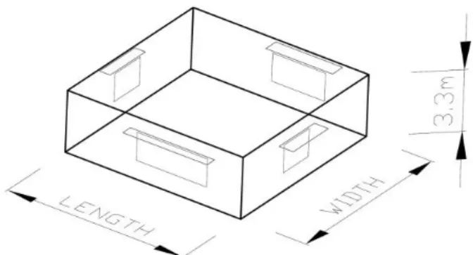
A simple model of a low-cost dwelling was established as shown in Fig.2. It is a rectangular parallelepiped - single thermal zone with four glazed windows on its four facades. Doors were intentionally omitted as their thermal properties were assumed to be similar to those of external walls. All internal partitions were considered as internal thermal mass. These partitions were not modelled in the airflow network, but their effects on airflow obstruction were estimated in the discharge coefficient of external windows. The floor area and height of the house are fixed at 100 m2 and 3.3 m, respectively. Only the building width and length are varied correspondingly. The house is assumed to be located in an urban area and occupied by maximum four people who share one gas stove (maximum heat dissipation of 250 W). The maximum lighting power is 1 kW. More details of the model are shown in Table 2 and Table3. It is worthy of note that optimal solutions of this simple model given by the optimization will indicate most appropriate design principles and parameters that can be considered the references for more sophisticated buildings.
Figure 2: Building model with variable building dimensions and openings
Two cases will be investigated. In the first case - NV case, the house is naturally ventilated (NV). The air flow rates are calculated by the airflow network model based on the hourly wind speed and the corresponding status of the openings. The outdoor wind speed profile follows an exponential function of height (exponent value 0.14) and the atmospheric boundary layer thickness is 270 m, similar to the terrain category 3 in ASHRAE handbook (ASHRAE 2009). In this case, windows and other openings are controlled by the occupants using some simple ventilation strategies. Table 3 shows six possible ventilation strategies which are commonly used in hot humid climates. The discharge coefficient of external windows was decided with care through a series of sensitivity analysis on this housing model. The results revealed that the simulation outputs and optimization results of this study were not sensitive to the variation of the discharge coefficient between 0.4 and 0.8. Based on the values found in the literature (Allard 1998), the discharge coefficient of 0.6 was selected. This value is slightly lower than a typical discharge coefficient for large openings due to the obstruction effect of internal partitions.
During the optimization process, some input variables of the airflow network model (building width/length ratio, area of each window and building orientation) changed from iteration to iteration. These changes were automatically updated in optimization input files by implementing some constraint functions in GenOpt (see variable constraints in Table 2). Furthermore, these changes continuously resulted in a secondary change of wind pressure coefficients on building facades. Each time the building configuration changes, the wind pressure coefficient corresponding to each wind direction must be recalculated. For rectangular building model in EnergyPlus, this heavy task can be done automatically by using the “surface average calculation” method proposed in (Swami and Chandra 1988).
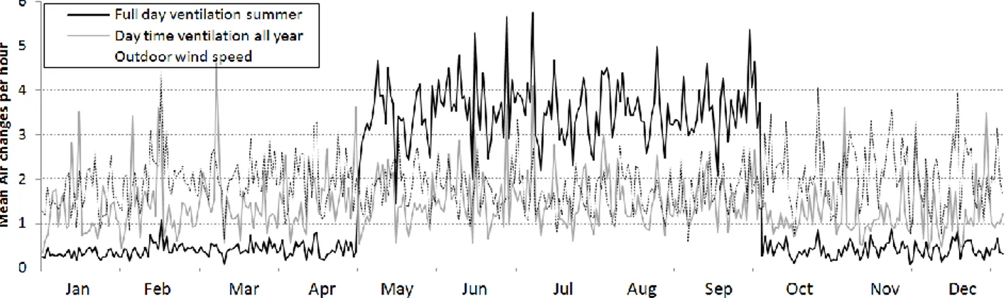
To control the operation of the airflow network, the predicted number of air changes per hour (ACH) in the house was examined. Fig. 3 shows predicted ACH of the model under different ventilation schemes. It can be seen that the ACH followed random fluctuations that tend to ‘mimic’ the effect of natural wind. Abrupt changes of the ACH at the start and the end of the summer period showed the impact of the ventilation scheme on the ACH. The predicted ACHs of this study were compared with experimental values of some similar cases as shown in Table 1. According to the range of ACH in these experiments, the predicted values of this study under all 3 ventilation schemes were rather reasonable. Hence, it can be said that the coupling of the airflow network model and the thermal simulation was able to provide adequate results of the airflow in the NV model.
Figure 3: Variations of predicted ACH in a year generated by the airflow network under the climate of Danang
Table 1: Mean predicted ACH of the airflow network model and results of some other experiments on natural ventilation
Mean outdoor wind speed (m/s) Measured ACH Predicted ACH References
Full day ventilation 1.75 3.25 This study
Day time ventilation 1.90 1.36
No ventilation 1.99 0.41
Isolated multi-zone detached house with 3 small openings in Austin, Texas, USA
3.5 7.45 (Lo and Novoselac
2012) Multi-zone townhouse in Reston, Virginia,
USA, winter and summer ventilation scheme
2.51 Not reported
0.62 1.25
(Wallace et al. 2002)
Isolated multi-zone detached house in Porto, Portugal
< 2.00 6.00 by
AIOLOS
(Allard 1998)
Multi-zone townhouse in Louvain la Neuve, Belgium
1.50 1.80
2.15 4.10 Apartment in Catania, Italy – single side
ventilation
2.60 2.30
Isolated two-zone detached house in Lyon, France (total volume: 68.64 m³)
1.60 1419 kg/h 1521 kg/h by COMIS
In the remaining case – AC case, the house is air-conditioned (AC) by an Ideal Loads Air System (ideal auto-sized HVAC system). This electric system works at 100% efficiency and is able to supply, without limit, the necessary heating or cooling supply air to meet heating or cooling load of the zone. A crucial parameter that needs to be correctly set is the infiltration rate in the AC case.
EnergyPlus provides a method which relates the air infiltration rate with outdoor conditions as follows:
2
* ( * * * )
i schedule outdoor outdoor
QI F A B T C V D V (1)
where:
Q is air infiltration rate (m3/s),
Ii is reference infiltration flow rate (m3/s). This value is varied during optimization process (Initial
value is 0.1),
Fschedule is hourly schedule, prescribed by user (from 0 to 1),
∆T (Tzone -Tout) is difference between indoor and outdoor temperature (ºC),
Voutdoor is hourly outdoor wind speed (m/s),
A, B, C and D are coefficients, prescribed by user,
Typical values for these coefficients are still subject to debate (Ernest Orlando Lawrence Berkeley National Laboratory 2010). Based on some parametric runs, we assumed (Fschedule, A, B, C, D) = (1.00, 0.00, 0.05, 0.18, 0.00). These coefficients produce a value of 0.026 m3/s (0.75 ACH) at ∆T of 2ºC and wind speed of 2 m/s, which corresponds to a typical summer condition in Hanoi.
3.2 Criteria for thermal comfort assessment and setpoints for HVAC system
Thermal comfort standards are required to help architects and building engineers to define an indoor environment in which a major part of building occupants will find thermally comfortable. The ‘steady state’ thermal comfort theory proposed by Fanger (Fanger 1970) in the early 1970s has become the foundation of international thermal comfort standards such as ISO 7730 (ISO 2005) and ASHRAE 55 (ASHRAE 2004) and has widely been used (Nguyen et al. 2012). However, field surveys have indicated that Fanger’s comfort model has failed to predict occupants’ thermal sensation in NV buildings in hot climates (Nguyen et al. 2012) where occupants often adapt themselves to the changes of outdoor weather by changing their behavior, adjusting their expectations and preferences. Recently, the adaptive comfort approach has emerged as an alternative method of thermal comfort assessment in such situations. Actually the adaptive comfort approach does not reject Fanger’s comfort theory, but it helps to clarify the mechanism through which people adapt themselves to the surrounding environment as well as provide a supplemental method to assess different thermal environments and situations. Due to the significance of these comfort theories, this study attempts to examine both of them in the light of simulation-based optimization.
There has been many adaptive comfort models developed during the last two decades. The model developed for hot humid South-East Asia (Nguyen et al. 2012) was chosen because it was based on the data collected within this region. This model defines the indoor comfort temperature Tcomf as a linear function of the mean monthly outdoor temperature Tout (Institute of Construction Science and Technology 2009) as follows:
0.341 18.83
comf out
T T (2)
The comfort range for 80% acceptability is nearly ± 3°C around Tcomf .
In the NV case, thermal performance of the house during a year is evaluated by mean Predicted Percentage Dissatisfied (PPD) index (Fanger 1970) (if Fanger’s comfort model is used) or Total Discomfort Hours (TDH) (if the adaptive comfort model is used). TDH is defined by total time of a year when indoor temperature is beyond the comfort range of equation (2). These long-term
assessments comply with the methods A and D in ISO 7730 (ISO 2005). To provide inputs for the calculation of PPD, hourly clothing insulation, work efficiency and activity of the occupants, indoor air velocity were estimated and assigned in EnergyPlus input files.
In the AC case, two types of cooling and heating setpoints for the HVAC system were examined, namely ‘fixed setpoints’ and ‘adaptive setpoints’. The ‘fixed setpoints’ were 20ºC and 26ºC. These values were intentionally chosen to maintain PPD index (Fanger 1970) of the indoor environment in most cases not to exceed 20% (80% acceptability, correspondingly). The ‘adaptive setpoints’ are the upper and lower boundaries of the comfort range defined by equation (2). Energy efficiency of the AC house is evaluated by the total energy consumption which is the sum of HVAC, equipments and lighting electricity.
The purpose of thermal comfort optimization is to minimize mean PPD or TDH. PPD is given in EnergyPlus outputs, but TDH is not included because current EnergyPlus versions do not support any user’s adaptive comfort models (the adaptive models of ASHRAE 55–2004 and EN15251 are newly accessible in EnergyPlus version 7.0). To implement the adaptive comfort model of South-East Asia into this tool, the paper proposed a method as described below:
- In each AC or NV thermal zone, an HVAC system was installed. In the NV thermal zone, this system was set at an extremely low capacity (heating and cooling air flow rates were 0.0001 m³/s) so that its heating and cooling effects do not have any influences on the zone and its energy consumption is negligible.
- By scheduling monthly heating and cooling setpoints, the adaptive setpoints were established.
- ‘Time heating setpoint not met’ and ‘Time cooling setpoint not met’ were called from the output dictionary of EnergyPlus (these outputs are only available if the thermal zone is equipped with HVAC systems). This output will give TDH or total time of a year temperature of the zone does not meet the criteria of the adaptive comfort model.
The purposes of these different types of setpoints were to examine their effects on the building life cycle cost (energy consumption) and on optimization results. It is necessary to emphasize that the percentage of satisfied occupants did not decrease if adaptive setpoints were imposed in AC office buildings (McCartney et Nicol 2002).
3.3 Parameters of designs and strategies considered in the optimization
As the present paper aims to optimize the passive designs of low-cost housing, 21 design parameters and 1 operational parameter were considered by a careful selection. All parameters to be optimized, variable constraints as well as their assigned values during the optimization process are listed in Table 2 and 3. All costs are given in USD.
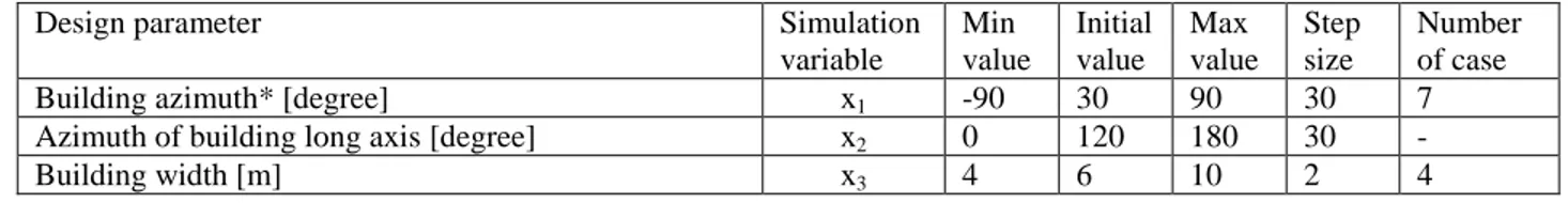
Table 2: Numerical variables and their design options (continuous variables)
Design parameter Simulation
variable Min value Initial value Max value Step size Number of case
Building azimuth* [degree] x1 -90 30 90 30 7
Azimuth of building long axis [degree] x2 0 120 180 30 -
Building length [m] x4 10 16.67 25 - -
Building shape ratio [dimensionless] x5 0.16 0.36 1 - -
South Window overhang size [m] x6 0.2 0.4 0.8 0.2 4
North Window overhang size [m] x7 0.2 0.4 0.8 0.2 4
East Window overhang size [m] x8 0.2 0.4 0.8 0.2 4
West Window overhang size [m] x9 0.2 0.4 0.8 0.2 4
South window width (height is fixed at 1.5m) [m] x10 1 2 4 1 4 North window width (height is fixed at 1.5m) [m] x11 1 2 4 1 4 East window width (height is fixed at 1.5m) [m] x12 1 2 3 1 3 West window width (height is fixed at 1.5m) [m] x13 1 2 3 1 3 External wall absorptance [dimensionless] x14 0.3 0.6 0.9 0.3 3 Reference infiltration flow rate (AC case) [m3/s] x15 0.05 0.1 0.15 0.05 3 Window crack infiltration (NV case) [kg/s-m] x15 0.002 0.004 0.006 0.002 3
Variables constraints
x2 - x1 = 90 x3 * x4 = 100 x3 / x4 = x5
*The angle between true North and the normal vector of the North-facing facade; clockwise is positive Table 3: Categorical design options and strategies (discrete variables)
Design parameter
Descriptions of design parameter Name in EnergyPlus Item cost ($/m2) Simulation variable Number of case External walls
110mm two-side plaster brick wall 100 20 x16 4
290mm two-side plaster brick wall with air gap 5cm
101* 26.5
two-side plaster brick wall with 2cm central insulation
102 33
two-side plaster brick wall with 4cm central insulation
103 38
Window type
Sgl Clr 6mm (single clear glazing 6mm) 200 45 x17 3
Sgl LoE (e2=.2) Clr 6mm (single clear glazing 6mm with loE film)
201* 70
Dbl Ref-A-L Clr 6mm/13mm Arg (double reflective glazings with 13mm Argon)
202 220
Roof type
Two-side plaster 120mm heavy RC 300 45 x18 3
Two-side plaster 120mm heavy RC with 2cm insulation
301* 52
Two-side plaster 120mm heavy RC with 4cm insulation 302 58 Ventila-tion strategy** (only for NV case)
Daytime ventilation summer 404 - x29 6
Daytime ventilation summer and mild seasons 405* -
Night Ventilation Summer 406 -
Night Ventilation Summer and mild seasons 407 -
Full day Ventilation summer 408 -
Full day Ventilation summer and mild seasons 409 - Floor
types
Concrete Slab tiled floor NO insulation 500 34 x20 3 Concrete Slab tiled floor with 2cm insulation 501* 39
Concrete Slab tiled floor with 4cm insulation 502 43 Thermal
mass
Thermal mass 110mm thickness 600 20 x21 3
Thermal mass 210mm thickness 601* 26
Thermal mass 410mm thickness 602 36.5
Total candidate solutions of the search-space were 7*6*48*38 ≈ 1.8*1010 cases. If parametric runs are used and each simulation takes approximately 3 minutes to complete, it takes 103077 years to examine all the search-space. It is obvious that the parametric runs cannot be applied in such extremely large search-space and the optimization becomes the only possible approach.
4. The choice of optimization algorithms for the present problem
The demand of a search-method that works efficiently on a specific optimization problem has led to various optimization algorithms. In most engineering optimization problems using the simulation-based approach, objective functions (simulation outputs) are generally non-linear, multi-modal, discontinuous and hence non-differentiable (Wetter and Polak 2004). Some algorithms developed for solving such problems fail to draw a distinction between local optimal solutions and global optimal solutions, and consider the former as final solutions to the problem. As an example, if the simulation program contains empirical assigned values (e.g. wind pressure coefficient), adaptive solvers with loose precision settings or iterative solvers using a convergence criterion, such as those in EnergyPlus, they may cause the cost function to be discontinuous. Hence gradient-based optimization algorithms, e.g. the Discrete Armijo Gradient algorithm (Polak 1997), that require smoothness of the cost function usually fail to reach the global minimum (Wetter and Wright 2004). As a result, the choice of optimization algorithm for a specific problem is crucial to yield the greatest reduction.
In this study, the problem is considered complex as it has 18 independent and 3 dependent variables to optimize. Wetter and Wright (Wetter and Wright 2004) compared the performance of 9 optimization algorithms and reported that for a detailed optimization problem, the hybrid algorithm (a combination of the particle swarm optimization (Eberhart and Kennedy 1995) and the Hooke-Jeeves algorithm (Hooke and Jeeves 1961)) achieved the biggest cost reductions but required a little more simulations than the standard genetic algorithm. The hybrid algorithm is a combination of the direct search optimization family and the stochastic population-based optimization family. The hybrid algorithm is capable to work efficiently since it performs a global search by the particle swarm optimization (PSO) and the Hooke–Jeeves algorithm then refines the search locally. This combination increases the possibility to get close to the global minimum rather than only a local one (Wetter and Wright 2004). On the other hand, as the PSO does not require the derivative of cost function because it is a population-based probabilistic optimization algorithm, it accepts both continuous and discrete variables of the cases in question. Therefore, the hybrid algorithm was first selected for comparative tests while the PSO was also considered as a reference algorithm during the optimization. Details of these algorithms can be found in GenOpt manual (Wetter 2009). The settings of these algorithms were identified through small trials and were almost by default (PSO: cognitive acceleration = 2.8, social acceleration = 1.3, maximum velocity gain = 0.5, constriction gain = 0.5; Hooke-Jeeves: mesh size divider = 2, initial mesh size exponent = 0, mesh size exponent increment = 1, number of step reduction = 4) except that we increased the number of particles per generation to 50 to match with the large search-space. The population size of 50 is expected to be large enough to allow the search to process from the first generation while it results in acceptable optimization time. The settings of the Hooke-Jeeves algorithm allow the optimization to refine the mesh of the continuous variables (parameter ‘step size’ indicated in Table 2) after the last evaluation of the PSO. These settings provide good optimization results with both standard benchmark functions and real-world applications using EnergyPlus as being tested in (Kampf et al. 2010). The number of generation was fixed at 200 for all optimizations. Our observations indicated that most optimization runs reached convergence after around 100 to 140 generations.
With the same settings, results of the comparative tests showed that the PSO needs much more time than the hybrid algorithm whereas the optimal solutions of the hybrid algorithm usually outperform those of the PSO. For these reasons, the hybrid algorithm was selected for the subsequent optimization. 5. The establishment of objective functions
The choice of a building design solution is a non-linear multi-objective optimization process, hence it often requires a trade-off among conflicting design criteria, e.g. the initial construction cost, the operating cost, and occupant’s thermal comfort (Wright et al. 2002). The most simplistic approach, namely “a priori’, is to assign a weight factor to each criterion, and then the objective function will be simply the weighted sum of the criteria. As an example, we consider an optimization problem of a thermal zone which consists of a construction cost function fc(X) and a
comfort performance function fp(X). These functions could be integrated into a single objective function by assigning two weight factors (a and b) or considering the second as a penalty function of the first: ( ) * ( ) * ( ) ( ) ( ) * ( ) c p c p f X a f X b f X or f X f X f X (3)
Another approach is to use the concept of Pareto optimality in which a set of trade-off solutions (Pareto set) is examined and appropriate solutions are then determined. In the present paper, the first approach was used to combine two design criteria into one objective function which consists of the construction cost and comfort performance; or the construction cost and the operating cost. We established two objective functions for the NV case and one for the AC case, based on two thermal comfort models: Fanger’s PMV-PPD model (Fanger 1970) and the adaptive comfort model (Nguyen et al. 2012) described earlier in section 3.2.
In the NV case, operating costs of different solutions is assumed to be similar; we, therefore, minimize the objective function I which consists of the construction cost and the comfort constraints: 4 ( ) ( ) * (1 ) or ( ) ( ) * ( / 8760) c c f x f x PPD f x f x TDH (4) where
fc(x) is total construction cost of the house,
is mean PPD of a year of the thermal zone in question. The exponent value of 4 was
determined after a few trials and errors and provided necessary comfort constraint on the construction cost.
To find the best combination of various design parameters in response to the climates, the objective function II was established to optimize occupant’s thermal comfort:
( ) or ( ) f x PPD f x TDH (5)
In the AC case, since the indoor thermal environment is controlled by the Ideal Loads Air System, we therefore optimize the life cycle cost of the house which consists of the initial construction cost and the 50-year operating cost. The demolition, transportation and waste management cost are assumed to be similar in all solutions. Thus the objective function III is the building Life Cycle Cost (LCC), defined as:
50
( ) c( ) o ( )
f x f x f x (6)
where
fc(x) is initial construction cost (present value), 50
( ) o
f x is total 50-year operating cost (present value).
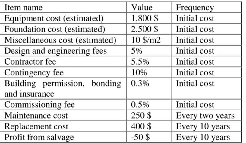
Using LCC provides an approach to combine the initial construction cost and the projected future costs into a single measure, called the “present value” (Ernest Orlando Lawrence Berkeley National Laboratory 2010). To include this into the analysis in EnergyPlus, we assumed an inflation rate of 2,5% per year, a discount rate of 1%, an electricity price escalation rate of 0.6% (the prices of electricity and various fuels do not change at the same rate as the inflation). Other annual maintenance cost, replacement cost and salvage cost are also included in the analysis (see Table 4). The current electricity price in Vietnam is 0.0728 $/kWh (EVN 2011). The initial construction cost is calculated by EnergyPlus based on estimated component costs (Ministry of Construction of Vietnam 2011) as listed in Table 3. Other secondary construction related costs, e.g. miscellaneous cost, design and engineering fees, contractor fee, contingency, permission, bonding and insurance, commissioning fee, equipment cost, foundation cost… are also taken into consideration in the analysis as shown in Table 4.
Table 4: Other costs and fees
Item name Value Frequency
Equipment cost (estimated) 1,800 $ Initial cost Foundation cost (estimated) 2,500 $ Initial cost Miscellaneous cost (estimated) 10 $/m2 Initial cost Design and engineering fees 5% Initial cost
Contractor fee 5.5% Initial cost
Contingency fee 10% Initial cost
Building permission, bonding and insurance
0.3% Initial cost
Commissioning fee 0.5% Initial cost Maintenance cost 250 $ Every two years Replacement cost 400 $ Every 10 years Profit from salvage -50 $ Every 10 years 6. Results and discussions
In the present study, there were 2 types of thermal comfort criteria used, 3 building sites and 3 objective functions. Hence there were totally 18 optimization runs. Full details of these optimization results are reported in the Appendix (categorized by building locations). For different analysis purposes, the Appendix could be categorized in 3 ways: by thermal comfort criteria; by building locations or by objective functions. The following sections discuss the findings from these results.
6.1 Effectiveness of the optimization approach
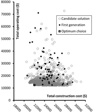
Fig. 4 shows the process of an optimization through which the optimal cost function III for Hochiminh city was found. Compared to the average of the first generation, the optimal design presents a reduction of 34.2% of the LCC while it still maintains a moderate construction price (22013 $). It also shows that the PSO in the hybrid algorithm performed a global search and quickly reached the potential optimal location.
The quantification of the optimization effectiveness needs a reference performance of an existing housing model which does not exist in our case. Therefore, the cost function values of the optimal solutions found by these optimizations were compared with the average and the best cost function of the first generation. The results are shown in Table 5. The average performance of the first generation which consists of 64 solutions is considered as a certain solution recommended by designers without performing an optimization. The best case of the first generation may be seen as the current best practice which reveals an estimation of the minimum reduction by the optimization.
Figure 4: Optimization effectiveness of a case in Hochiminh city - graphical assessment Table 5: Percentage reduction of objective function value by the optimizations
Objective function Location Optimal solution
Compared with the first generation Best solution Min reduction (%) ‘Average’ solution Average reduction (%) Mean PPD (objective function II) Hanoi 41.5 46.7 11.1 55.8 25.7 Danang 33.8 42.1 19.7 57.0 40.7 Hochiminh 54.4 61.2 11.1 79.1 31.2
Total discomfort hours (objective function II)
Hanoi 1501 2335 35.7 3388 55.7
Danang 58 792 92.7 2109 97.2
Hochiminh 18 970 98.1 3595 99.5
LCC using fixed setpoints (objective function III)
Hanoi 46405 59136 21.5 90007 48.4
Danang 47174 59472 20.7 95985 50.9
Hochiminh 49957 65981 24.3 112945 55.8
LCC using adaptive
setpoints (objective function III)
Hanoi 39908 42607 6.3 60561 34.1
Danang 35047 36940 5.1 51053 31.4
Hochiminh 34468 36560 5.7 52390 34.2
The analysis in Table 5 indicates that the optimization method can be seen as an effective decision support tool that helps designers in preliminary design stages. The optimization approach sometimes reduces the objective cost significantly, possibly up to 99.5%, and potentially provides
0 10000 20000 30000 40000 50000 60000 70000 80000 To tal ope rat ing cos t ($)
Total construction cost ($) Candidate solution First generation Optimum choice
the optimal solution (or at least, the solutions near the optimum). Compared with the average performance of normal designs without optimization, the reductions were no less than 25.7%. The minimum reduction varied in a very wide range, but it was no less than 5.1%. In the NV house, the optimization yielded great reductions if the adaptive thermal comfort was chosen as the thermal constraint. The optimal houses in Danang and Hochiminh city are nearly comfortable all year round without HVAC systems.
Currently the simulation-based optimization process seems rather sophisticated as it requires manual coupling of the optimization programme and the building simulation tool. However, this difficulty is expected to overcome soon when the optimization algorithms will be integrated into building simulation tools.
6.2 The role of adaptive comfort setpoints in energy saving
The optimization using the objective function III was aimed to examine the effect of different thermal comfort criteria on building energy consumption through the whole building life cycle. As can be seen from Table 5, the adaptive setpoints applied in the HVAC system would offer a significant reduction in the building LCC. LLCs of the optimal houses were reduced 14% (case Hanoi), 26% (case Danang) and up to 31% (case Hochiminh city), compared with those using the fixed-setpoints. These reductions are more significant than many other energy saving measures. It can be seen that the benefits given by adaptive setpoints increase from the North to the South corresponding to the increase of annual average temperature - from 23.6°C to 25.8°C and to 27.4°C, respectively. The benefits of adaptive setpoints in buildings in temperate and cold climates (e.g. in Netherlands and Finland) were questioned by some studies (Sourbron and Helsen 2011, Hamdy et al. 2011) as unexpected results were detected. However, in hot climates the adaptive comfort theory allows higher acceptable indoor temperatures, thus it tends to reduce cooling energy. Earlier studies (Tøftum et al. 2009, McCartney and Nicol 2002) also indicated that buildings using thermal setpoints in compliance with the adaptive comfort model may result in significant energy savings. Notably, the adaptive thermal setpoints in AC office buildings do not interfere with occupant’s thermal satisfactory (McCartney and Nicol 2002). This finding also seems true in residential facilities where occupants often have more adaptive opportunities, e.g. changing clothing, opening control, activities. Hence the adaptive approach also further questions the validity of applying fixed thermal setpoints to a real living environment, especially in hot climates.
6.3 Deviation of optimal solutions found by different thermal comfort criteria
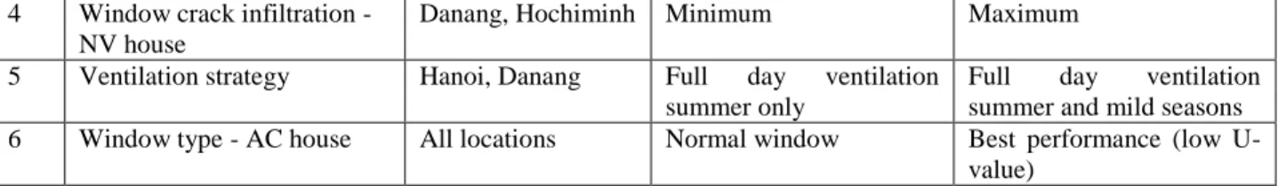
The results in the Appendix were categorized by the comfort models applied. In general, the optimal solutions of these two comfort models were found rather similar although there were a few discrepancies as listed in Table 6. These discrepancies were mainly caused by more stringent requirements on the indoor surface temperature and humidity of Fanger’s comfort model. More ventilation is needed to remove the humidity generated by human occupancies (discrepancy no. 3; 4; 5) and other measures (no.1; 2; 6) ensure stable surface temperature, especially glazed surfaces. Table 6: Discrepancies between the optimal solutions generated by two thermal comfort criteria No. Discrepancy Found in Adaptive comfort model Fanger’s comfort model
1 Building azimuth Hochiminh -21° 15°
2 North and South window overhang
All locations Small overhang (in most cases)
Largest overhang (in most cases)
3 North and South window width - NV house
4 Window crack infiltration - NV house
Danang, Hochiminh Minimum Maximum
5 Ventilation strategy Hanoi, Danang Full day ventilation summer only
Full day ventilation summer and mild seasons 6 Window type - AC house All locations Normal window Best performance (low
U-value)
Although only a few discrepancies were observed in each city, comfort performances of the optimal solutions were contradictory. As shown in Table 5, the optimal
PPD
of Hanoi, Danang and Hochiminh were 41.5%, 33.8% and 54.4%. This means that none of these houses is thermally acceptable. Meanwhile, the optimal TDH of Danang and Hochiminh were nearly perfect (58 and 18 hours per year, respectively). Hanoi, by any criteria, always needs heating-cooling systems to maintain thermal comfort during a year. Our experience about adaptive thermal comfort and housing study in hot humid climate indicates that Fanger’s comfort model has failed to predict the thermal sensation of occupants living in NV buildings. Fanger’s PMV-PPD model cannot take into account complex human interactions with the surrounding environment by changing their behaviour and slowly getting adapted by adjusting their expectations and preferences (Nguyen etal. 2012). Therefore, this study is in favour of the adaptive comfort approach for the optimization
of NV buildings.
6.4 Differences between the optimal NV and AC houses
Figure 5: Optimal combination of variables for the best thermal comfort condition (NV house) 0 0.1 0.2 0.3 0.4 0.5 0.6 0.7 0.8 0.9 1 N o m al iz ed val ue o f var iab le
s Hanoi-adaptive comfort Danang-adaptive Hochiminh-adaptive
0.0 0.2 0.4 0.6 0.8 1.0 N o m al iz ed val ue o f var iab le s
Hanoi-adaptive comfort Hanoi-fixed setpoints Danang-adaptive Danang-fixed setpoints Hochiminh-adaptive Hochiminh-fixed setpoints
Figure 6: Optimal combination of variables for the best Life Cycle Cost (AC house)
The optimization results in the Appendix were categorized by the objective functions and presented in Fig. 5 and Fig. 6. The results of objective function II and III represent the optimal designs of the NV and AC houses, respectively. As expected, there were some differences between these two housing categories as shown in Table 7. Among these, a few important design parameters are contradictory, e.g. building shape and thermal mass. The internal thermal mass is only required in the NV case, maybe for night pre-cooling when night ventilation is applied. Shapes of the AC house should be square or near square while an East-West long rectangular geometry is suitable for the NV house. These indicate that designers should take building environmental control methods, e.g. NV or AC, into consideration to propose an adequate design in the early stage of a project.
Table 7: Differences of optimal NV and AC buildings
Design parameter NV building AC building
Building shape Long rectangular Nearly square
North window overhang Almost maximum Varied
Indoor thermal mass Maximum Minimum
Window type, external wall type, roof type Best performance (low U-value) Varied
North and South window overhang Large overhang (in most cases) Small overhang (in most cases) The objective function I and II did not give the same solutions because the comfort criteria were combined with the construction cost in the objective function I. With the balance between the comfort and the investment, the solutions generated by the objective function I seem more favourable for low income residents. The objective function III should be used for AC buildings while the objective function II seems useful for the design of net-zero energy houses or passive houses.
6.5 General recommendations for each location in response to the local climate
The results in the Appendix were categorized by building locations to examine the effect of the climate on building designs. Fig. 7 shows some basic climate data of three regions. Hanoi has a sub-tropical climate with fairly dry cold winters and hot summers, but the lowest temperature hardly falls below 5°C. In Danang, the climate is basically tropical monsoon with very short and warm winters. The lowest temperatures is often well above 15°C. Hochiminh city has a typical hot and humid climate. There are one dry and one rainy season, corresponding to two monsoons regimes throughout the year.
Figure 7: Basic climate data of Hanoi, Danang and Hochiminh city
In all regions, the optimal solution is a combination of: (1) small East and West windows with largest overhangs; (2) low thermal absorptance of external walls: bright colour, for example; (3) good air tightness; (4) no floor insulation to facilitate heat exchange with the earth; (5) maximum thermal mass in NV cases and minimum thermal mass in AC cases; (6) Full day ventilation under warm or hot weather; (7) minimum window areas in AC cases. General recommendations for each region were also derived. In Hanoi, the house should be nearly square; the building azimuth should be within 0° and -7.5° with a moderate or large South window in NV cases, a well-insulated roof and external walls. In Danang, the house needs short South window overhangs, a well-insulated roof; the building shape follows the building types (NV or AC) and the building long axis should be shifted to an East-West orientation. The solutions for Hochiminh city are not quite explicit because of the disagreement among solutions, thus these should be based on specific situations of the project.
It can be seen that among the optimal solutions, the discrepancies always exist. It is mainly because of the contradiction between the cost and the comfort criteria. For example, the objective function I found elements at the lowest cost but poor thermal performance that were usually rejected by comfort-related objective functions. It reveals that the objective function has a great influence on the optimal solution found and thus designers’ decisions.
7. Conclusion
This paper fully describes a process to optimize LCH design using the simulation-based optimization method. The characteristics of a low-cost dwelling and its operation were reproduced by a simplified single-zone thermal model in EnergyPlus. In particular, the airflow network model was applied to simulate natural wind driven ventilation in the house. The optimal LCH models were carefully examined through 18 optimizations of 3 objective functions, including 2 thermal comfort models, 2 building running modes under 3 climates.
The optimal results generated by the two comfort models were not identical. Based on the results of many earlier studies on thermal comfort, this study is in favour of the optimization results given by the adaptive comfort model. The adaptive comfort setpoints for HVAC system shows a considerable potential of energy saving without any drop in thermal comfort levels through the
whole 50-year life cycle of the house. The cost saving in Vietnam depends on the climate and may be as high as 14% to 31%, compared with the fixed setpoints. Hanoi, by any criteria, always needs air-conditioning systems to maintain comfort during a year whereas Danang and Hochiminh may entirely rely on passive designs and strategies. The optimal combinations for the design of LCH in each climatic region were also recommended.
The optimization results show that the optimal designs of a naturally ventilated house and an air-conditioned one had some differences, and even in a few categories, they were contradictory. Therefore, the building environmental control method must be initially considered to create adequate proposals in the early stage of the project.
The study also shows the considerable potential of the optimization method in energy saving, life cycle cost and comfort improvement. The benefit given by the simulation-based optimization is actually remarkable while the computational cost is gradually decreased by advances in computational technologies. Since the work to couple EnergyPlus - GenOpt and then to define the optimization problems takes only a few hours, the optimization method shows a very promising applicability and can yield considerable economic gains.
In this work, the presence of internal partitions was modelled in the airflow network by assuming a reduced discharge coefficient of the external windows. This assumption was however subject to some uncertainties because of the fact that the discharge coefficients of large openings found in the literature are somewhat inconsistent and that the distribution of internal partitions may vary from case to case. In the paper, the predicted air flow rates were qualitatively compared with the values of the earlier studies. It is therefore necessary to emphasize that the reliability of this approach needs to be validated by more robust methods, e.g. wind tunnel experiments or full-scale measurements of air flow rates.
Appendix
All optimization results categorized by building locations (Refer to Table 2 and 3 for details about the parameters x1, …, x21) Comfort model Objective function Location Optimum cost x1 x3 x6 x7 x8 x9 x10 x11 x12 x13 x14 x15 x16 x17 x18 x19 x20 x21 Adaptive I Hanoi 5385 0 9.13 0.65 0.35 0.8 0.8 4 1 1 1 0.3 0.002 103 200 302 408 500 600 II Hanoi 1501 0 7 0.8 0.8 0.8 0.8 2.5 1 1 1 0.6 0.002 103 202 302 408 500 602 III Hanoi 39908 0 9.88 0.2 0.2 0.8 0.8 1 1 1 1 0.34 0.05 103 201 302 ---- 500 600 Fanger I Hanoi 96170 -7.5 8.75 0.54 0.24 0.8 0.8 2 1 1 1 0.3 0.002 100 200 301 409 500 600 II Hanoi 41.5 -7.5 8 0.8 0.8 0.8 0.8 3.5 1 1 2 0.3 0.002 103 202 302 409 501 602 III Hanoi 46405 0 9.38 0.8 0.61 0.8 0.8 1 1 1 1 0.3 0.05 103 202 302 ---- 500 600 Adaptive I Danang 199 0 4 0.2 0.4 0.8 0.8 1 1 1 1 0.3 0.002 103 202 302 408 500 602 II Danang 58 -7.5 4 0.2 0.65 0.8 0.8 1 1 1 1 0.3 0.002 103 202 302 408 500 602 III Danang 35047 0 9.25 0.2 0.39 0.8 0.8 1 1 1 1 0.3 0.05 101 200 301 ---- 500 600 Fanger I Danang 74022 0 8.5 0.8 0.75 0.8 0.8 2 2 1 1 0.3 0.006 100 200 300 409 500 600 II Danang 33.8 0 4 0.8 0.8 0.8 0.8 4 4 1 1.5 0.3 0.006 101 202 302 409 500 602 III Danang 47174 0 9.25 0.8 0.8 0.8 0.8 1 1 1 1 0.3 0.05 103 202 302 ---- 500 600 Adaptive I Hochiminh 60 -21 4 0.2 0.75 0.8 0.8 1 1 1 1 0.3 0.002 103 202 302 409 500 602 II Hochiminh 17.8 -21 4 0.5 0.8 0.8 0.8 1 1 1 1 0.3 0.002 103 202 302 409 500 602 III Hochiminh 34468 -3.8 9.5 0.33 0.43 0.8 0.8 1 1 1 1 0.3 0.05 101 200 301 ---- 500 600 Fanger I Hochiminh 118474 15 8.5 0.8 0.7 0.8 0.8 1 1 1 1 0.3 0.006 100 200 300 409 500 600 II Hochiminh 54.4 15 4 0.8 0.8 0.8 0.8 4 2.63 1 3 0.3 0.006 100 202 300 409 500 600 III Hochiminh 49957 0 9.38 0.8 0.8 0.8 0.8 1 1 1 1 0.3 0.05 103 202 302 ---- 500 600
References
Adams, B.M., Bohnhoff, W.J., Dalbey, K.R., Eddy, J.P., Eldred, M.S., Gay, D.M., Haskell, K., Hough, P.D., Swiler, L.P., 2009. DAKOTA, A Multilevel Parallel Object-Oriented Framework for Design
Optimization, Parameter Estimation, Uncertainty Quantification, and Sensitivity Analysis: Version 5.0 User's Manual, Sandia Technical Report SAND2010-2183 (Version 5.2).
Allard, F., 1998. Natural ventilation in buildings – A design Handbook. London: James & James.
ASHRAE, 2004. ASHRAE standard 55-2004: Thermal Environmental Conditions for Human Occupancy, ASHRAE, Atlanta.
ASHRAE, 2009. ASHRAE Handbook of Fundamentals. Atlanta GA: ASHRAE, Inc..
Central Population and Housing census Steering Committee, 2010. The 2009 Vietnam population and
housing census: completed results. Hanoi: Statistical Publishing House.
Crawley, D.B.; Lawrie, L.K.; Winkelmann, F.C.; Buhl, W.F.; Huang, Y.J.; Pedersen, C.O.; Strand, R.K.; Liesen, R.J.; Fisher, D.E.; Witte, M.J.; Glazer, J., 2001. EnergyPlus: creating a new-generation building energy simulation program. Energy and Buildings, 33 (4), 443–57.
Eberhart, R.C. and Kennedy J., 1995. A new optimizer using particle swarm theory. Nagoya: Proceedings of the Sixth International Symposium on Micro Machine and Human Science.
Ernest Orlando Lawrence Berkeley National Laboratory, 2010. The Encyclopedic Reference to EnergyPlus
Input and Output - Version October 2010. Berkeley: Lawrence Berkeley National Lab.
EVN, 2011. Vietnam electricity price [online]. EVN. Available from: www.evn.com.vn/Default.aspx?tabid=59&language=en-US [Accessed 10th August 2011].
Fanger, P.O., 1970. Thermal comfort. Copenhagen: Danish Technical Press.
Hamdy, M., Hasan, A., and Siren K., 2011. Impact of adaptive thermal comfort criteria on building energy use and cooling equipment size using a multi-objective optimization scheme. Energy and Buildings, 43, 2055-2067.
Hooke, R. and Jeeves. J., 1961. ‘Direct Search’ Solution of Numerical and Statistical Problems. Journal of
the Association for Computing Machinery, 8 (2), 212-229.
Hopfe, C.J. and Hensen, J.L.M., 2011. Uncertainty analysis in building performance simulation for design support. Energy and Buildings, 43, 2798–2805.
Institute of Construction Science and Technology, 2009. Vietnam Building Code 2009 - QCVN 02:
2009/BXD - Natural Physical & Climatic Data for Construction. Hanoi: Ministry of Construction of
Vietnam.
ISO, 2005. ISO 7730-2005: Ergonomics of the thermal environment - Analytical determination and interpretation of thermal comfort using calculation of the PMV and PPD indices and local thermal comfort criteria. Geneva: ISO.
Lo, L.J.; Novoselac, A., 2012. Cross ventilation with small openings: Measurements in a multi-zone test building. Building and Environment, 57, 377-386
Kampf, J.H., Wetter, M. and Robinson, D, 2010. A comparison of global optimisation algorithms with standard benchmark functions and real-world applications using EnergyPlus. Journal of Building
Performance Simulation, 3, 103-120.
McCartney, K.J. and Nicol, J.F., 2002. Developing an adaptive control algorithm for Europe. Energy and
Ministry of Construction of Vietnam, 2011. Construction price 09 August 2011 [online]. MOC. Available from: www.moc.gov.vn [Accessed 10th August 2011].
Nguyen, A.T., Singh, M.K. and Reiter S., 2012. An adaptive thermal comfort model for hot humid South-East Asia. Building and Environment, 56, 291-300.
Office of Energy Efficiency and Renewable Energy (U.S. Department of Energy), 2012. EnergyPlus
Energy Simulation Software - Testing and validation [online]. Available from http://apps1.eere.energy.gov/buildings/energyplus/energyplus_testing.cfm [Accessed 6th August 2012].
Polak, E., 1997. Optimization, Algorithms and Consistent Approximations. Applied Mathematical
Sciences, 124, 779.
Sourbron, M. and Helsen L., 2011. Evaluation of adaptive thermal comfort models in moderate climates and their impact on energy use in office buildings. Energy and Buildings, 43, 423–432.
Swami, M. V. and S. Chandra., 1988. Correlations for pressure distribution on buildings and calculation of natural-ventilation airflow. ASHRAE Transactions, 94 (Pt 1), 243-266.
Tøftum, J., Andersen, R.V. and Jensen, K.L., 2009. Occupant performance and building energy consumption with different philosophies of determining acceptable thermal conditions. Building and
Environment, 44, 2009–2016.
Wallace, L.A. ; Emmerich, S.J. ; Howard-Reed, C., 2002. Continuous measurements of air change rates in an occupied house for 1 year: The effect of temperature, wind, fans, and windows. Journal of
Exposure analysis and Environmental Epidemiology, 12, 296-306
Walton, G.N., 1989. Airflow network models for element-based building airflow modeling. ASHRAE
Transaction, 95 (2), 611–620.
Wetter, M., 2001. GenOpt, A generic optimization program. Rio de Janeiro: Proceedings of IBPSA's Building Simulation 2001 Conference.
Wetter, M., 2009. GenOpt, Generic optimization program - User manual, version 3.0.0. Technical report
LBNL-5419. Berkeley: Lawrence Berkeley National Lab.
Wetter, M. and Polak, E., 2004. A convergent optimization method using pattern search algorithms with adaptive precision simulation. Building Services Engineering Research and Technology, 25 (4), 327– 338.
Wetter, M. and Wright, J.A., 2004. A comparison of deterministic and probabilistic optimization algorithms for nonsmooth simulation-based optimization. Building and Environment, 39, 989–999. Wright, J.A., 1994. Optimum Sizing of HVAC Systems by Genetic Algorithm. Liege: Proceedings of the
4th International Conference on System Simulation in Buildings.
Wright, J.A., 1986. The optimised design of HVAC systems. Thesis (PhD). Loughborough University of Technology.
Wright, J.A., Loosemore, H.A. and Farmani, R., 2002. Optimization of Building Thermal Design and Control by Multi-Criterion Genetic Algorithm. Energy and Buildings, 34 (9), 959-972.