HAL Id: hal-01154692
https://hal.archives-ouvertes.fr/hal-01154692
Submitted on 22 May 2015
HAL is a multi-disciplinary open access
archive for the deposit and dissemination of
sci-entific research documents, whether they are
pub-lished or not. The documents may come from
teaching and research institutions in France or
L’archive ouverte pluridisciplinaire HAL, est
destinée au dépôt et à la diffusion de documents
scientifiques de niveau recherche, publiés ou non,
émanant des établissements d’enseignement et de
recherche français ou étrangers, des laboratoires
Inflation and bending of an orthotropic inflatable beam
Quang-Tung Nguyen, Jean-Christophe Thomas, Anh Le Van
To cite this version:
Quang-Tung Nguyen, Jean-Christophe Thomas, Anh Le Van. Inflation and bending of an orthotropic
inflatable beam. Thin-Walled Structures, Elsevier, 2015, pp.129-144. �10.1016/j.tws.2014.11.015�.
�hal-01154692�
INFLATION AND BENDING OF AN ORTHOTROPIC
INFLATABLE BEAM
Quang-Tung NGUYENa, Jean-Christophe THOMASb, Anh LE VANb aUniversity of Danang, University of Science and Technology,
54 Nguyen Luong Bang Street, Lien Chieu District, Da Nang, Vietnam bLUNAM Université, Université de Nantes-Ecole Centrale Nantes, GeM (Institute for Research in Civil and Mechanical Engineering), CNRS UMR 6183,
2, rue de la Houssinière, BP 92208, 44322 Nantes Cedex 3, France
Abstract
An inflatable beam is an airtight structure made of a soft technical fabric and sub-jected to an internal pressure which gives it a final cylindrical shape, a pre-stress in the membrane and a bearing capacity. Against all appearances, it is not a standard beam and it requires a specific formulation in order to take account of the internal pressure which plays a key role in its mechanical response.
This work deals with inflatable beams made of orthotropic materials. The first part of the paper is concerned with the inflation of the membrane tube, an important stage which is often neglected so far in the literature. As preliminaries of the bending prob-lem studied in the next part of the paper, the constitutive law related to the inflated state of the tube – not the natural state – is investigated. It will be shown that the consti-tutive law related to the inflated pre-stressed state is not the same as the consticonsti-tutive law related to the natural state. Expressions of the material coefficients involved in the former constitutive law will be established from the material coefficients defined on the natural reference configuration which are the only ones supposed to be known. The second part of the paper deals with the bending of the inflatable beam. The Tim-oshenko beam kinematics will be chosen because of the significant shear effect in the tube wall and the problem will be formulated in finite deformations in order to accounts for all the nonlinear effects, in particular the action due to the internal pressure which is a follower load. The nonlinear system of equations obtained will then be linearized around the pre-stressed configuration and will result in a more tractable linear system.
The proposed formulation allows a comprehensive study of the influence of the internal pressure on the geometry and material properties of orthotropic inflatable beams The analytical results will be compared with numerical results obtained from a nonlinear membrane finite element code.
Key words: Inflatable beam; membrane tube; orthotropy; inflation; bending
1. INTRODUCTION
Inflatable structures made of modern textiles have been used for several decades. Among their applications in space industry, there are deployable antennas, inflatable re-entry capsules and inflatable solar power sails, mainly made of isotropic fabrics. The inflatable technology is also widely applied to terrestrial structures, both in civilian and military fields. Today, large inflatable structures are built for sports centres , exhibition halls and storage shelters. The fabrics used in these types of structures are often made of warp and weft threads which ensure the mechanical resistance and a coating which ensures the airtightness. In comparison with conventional structures, the inflatable structures may present some advantages in some specific cases: they are light, easily foldable, easily to transport, deploy. Moreover, it is not very expensive to manufacture them and keep them deployed.
The pressurized membrane structures are often made of bearing components which take the shape of tubes or beams. Each component is made of an airtight fabric and subjected to an internal pressure which gives it a final cylindrical shape, a pre-stress in the membrane and a bearing capacity. In the sequel, mention will be made of two types of reference configuration:
(i) the natural configuration, where there is no external loads and the stress field is zero. The geometry and material properties are supposed to be known in the natural configuration. The membrane has no bearing capacity in this state;
(ii) the pre-stressed configuration, where the membrane structure is subjected to the internal pressure only. The geometry and, as will be seen below, the material properties are different from those in the natural state. The bearing capacity of the structure should increase with the pre-stress, i.e. with the internal pressure.
Several works have been conducted in the literature to predict the behavior of an inflated tube subjected to bending loads. In these works, the reference configuration corresponds to the pre-stressed configuration of the inflated tube.
The earliest analytical expressions for the load-deflection response and the collapse load of a cantilever pressurized membrane tube can be found in Comer and Levy’s pa-per [1]. In this work, the usual Euler-Bernoulli kinematics was chosen and it was assumed that the tube is made of an isotropic linear elastic material. Later, Webber [2] extended Comer and Levy’s theory [1] to the case of a tube subjected to bending and twisting, and succeeded in determining how a twisting moment modifies the de-flection, the wrinkling load as well as the collapse load. Afterwards, Main et al. [3] improved Comer and Levy’s theory of pressurized membrane tubes [1] by considering the effect of the bi-axial stress state on the wrinkling. Experiments were conducted on pressurized tubes with circular cross-sections and the results obtained were com-pared with those given by Comer and Levy’s theory [1]. In another study, Main [4] took the orthotropic property of the fabric into account so as to enhance his previously developed theory. Suhey et al. [5] carried out numerical computations on anisotropic pressurized membrane tubes by means of membrane finite elements and validated their finite element model by comparing their numerical results with Main et al.’s theoretical results in [3],[4].
When using the Euler-Bernoulli kinematics, the internal pressure does not appear in the expression of the deflection. In order to improve the previous formulations, many other authors preferred to use the Timoshenko kinematics which is more appropriate for thin-walled beams.
A major contribution in this formulation type is due to Fichter [6] who developed a theory for pressurized cylindrical membrane tubes made of isotropic membrane. His approach was based on the minimization of the total potential energy. After lineariza-tion, Fichter successfully derived the analytical equations for the bending problem of a pressurized membrane tube, exhibiting the very term of the internal pressure in the deflection expression.
Steeves [7] adopted a similar approach and proposed solutions in terms of Green functions. Wielgosz and Thomas [8] [9] dealt with analytical solutions for inflatable
isotropic beams and panels by establishing the equilibrium equations in the deformed state in order to incorporate the internal pressure in their formulation. They considered the internal pressure as a follower force which represents the strengthening effect on the bending and shear stiffnesses. Le van and Wielgosz [10] improved Fichter’s theory [6] by using the virtual power principle in the context of the total Lagrangian formulation. They considered large displacements and rotations in order to take account of all the nonlinear terms in the kinematic and equilibrium equations, and proposed solutions for the bending and buckling of a pressurized isotropic membrane tube. Davids and Zhang [11] confirmed Fichter’s results by considering the pressure work during the volume change in isotropic Timoshenko beams. On the basis of [10], Apedo et al. [12], Nguyen et al. [13] went further by developing a theory for pressurized membrane tube made of an orthotropic material. They first used a 3D kinematics and then linearized their formulation. The bending and buckling problems were investigated, and the results obtained show that it is essential to consider the fabric orthotropy in the computations. In all the above-mentioned works, the reference configuration is the pre-stressed configuration, yet the material coefficients used in the constitutive law are those related to the natural configuration, which corresponds to the tube without internal pressure. On the other hand, studies on the behavior of fabrics used in pressurized membrane structures have shown the fabric characteristics in the pre-stressed state differ from those in the natural state and depend on the internal pressure.
Cavallaro et al. [14] utilized finite element analysis to compute the load-displacement curve of a pressurized membrane tube subjected to four-point bending conditions and found that the mechanical response strongly depends on the internal pressure. Turner et al. [15] conducted torsion tests on pressurized membrane tubes subjected to different internal pressures with the aim of determining the shear modulus of the fabric in the pre-stressed configuration. Their experimental results also reveal that the shear modu-lus depends on the internal pressure and the larger the pressure is, the larger the shear modulus. Later on, Davids and Zhang [11] realized four-point bending tests with the same fabric as in [15] and with different internal pressures. By taking the shear mod-uli in [15], these authors performed an inverse analysis upon the load-displacement and obtained the Young’s modulus. They noticed that the Young’s modulus of the
fabric in the pre-stressed configuration increases with the internal pressure. A beam finite element was designed to compute the load-displacement response of the pres-surized membrane tube and the input data used were the material coefficients in the pre-stressed configuration of the structure. A good correlation found between the nu-merical model and the experimental deflection indicated that it is essential to use the material coefficients related to the pre-stressed configuration. More recently, Kabche et al. [16] presented a complete procedure based on Turner et al.’s test [15] in order to quantify the fabric properties in the pre-stressed configuration, which are strongly dependent on the internal pressure. They also realized the same four-point bending test as Davids and Zhang [11] and made similar observations on the material coefficients related to the pre-stressed configuration.
Inflatable structures are usually made of coated woven fabrics, which mostly dis-play an anisotropic and viscoelastic behavior. In most of the above-mentioned studies, coated fabrics are modeled - as commonly practiced in the field of tensile structures - as orthotropic membranes under the plane stress assumption. Accordingly, we will not deal here with fabrics but with orthotropic membranes and we will assume that the membrane obeys the Saint Venant - Kirchhoff orthotropic elastic law. Elaborate mod-els of coated fabrics and comparison with experimental results are much more complex subjects and they will not be considered in this paper. Our aim is to propose a compre-hensive analytical model for orthotropic inflatable beams including both the inflation and the bending stages. The paper is organized as follows:
• Section 2 defines the problem of a pressurized membrane tube and points out that one should consider two distinct successive stages. The first is the inflation of the membrane tube, an important stage which is often neglected so far in the literature. The second stage is the bending of the pressurized membrane tube and it will be seen further that the results of this stage strongly depend on those acquired in the first stage.
• Sections 3 to 5 are concerned with the inflation of the membrane tube. Section 3 is a brief reminder of the analytical results given in [17] for the geometry of the inflated tube. As preliminaries of the bending problem studied in the next part
of the paper, the constitutive law related to the inflated state of the tube – not the natural state – is investigated in Section 4. It will be shown that the tube remains orthotropic with respect to the inflated state. However, the material coefficients involved in the constitutive law are no longer the same. As far as the authors’ knowledge, this is the first time a bridge is established between the material coefficients at the natural state and those at the pressurized state. The change of the material coefficients are numerically computed on different geometries of the tube and material properties of the membrane in Section 5. The values of the material coefficients for the membrane will be chosen of the same order as the coefficients found in the literature for fabrics. The numerical results obtained will be used in the bending stage of the tube.
• The last part of the paper – Sections 6 to 9 – deals with the bending of the tube. As will be described in Section 6, the Timoshenko beam kinematics is chosen because of the significant shear effect in the tube wall and the problem is formu-lated in finite deformations in order to accounts for all the nonlinear effects, in particular the action of the internal pressure which is a follower load. The result of this is a nonlinear system of equations governing the bending problem, which highlights the significant role of the internal pressure in the response of inflat-able beams. In the next Section 7, the nonlinear system of equations obtained will be linearized around the pre-stressed configuration and will result in a more tractable linear system. Finally, Sections 8 and 9 constitute an application of the obtained analytical results to a cantilever inflatable beam. The numerical results for different tube geometries, materials and internal pressures will be compared with numerical results obtained from a nonlinear membrane finite element code.
2. THE PROBLEM OF THE PRESSURIZED MEMBRANE TUBE
The problem will be described using a kinematical time t which is not necessarily the physical time as one is in Statics, and which is useful, however, to relate the suc-cessive states of the mechanical system. When studying the bending of a pressurized
membrane tube, one has to consider two successive stages, formulated in two different ways and based on two different reference configurations (see 1).
1. The inflation stage. It is assumed that there exists a time t∅when no external loading is applied on the tube and the stress field therein is zero. At that time, the tube is said in the stress-free (or natural) configuration (or state).
The typical feature of a membrane tube is that the tube has no stiffness in the absence of external loading and the only way for it to acquire a stiffness is to subject it to an internal pressure. Thus, the inflation is essential to membrane structures and deserves a separate study on its own, where the only loading is the internal pressure. The inflation stage will be formulated as a three-dimensional problem of nonlinear elasticity. The reference configuration will be chosen as the stress-free one and referred to as the natural reference configuration. 2. The bending stage. The internal pressure causes pre-tensions in the tube wall
and enables the tube to bear other external loads. From a given time t0> t∅, the
internal pressure is kept fixed and other loads are then applied on the external surface in order to bend the tube.
The bending problem will be formulated using a Timoshenko kinematics with finite displacements and rotations. This time, the reference configuration is cho-sen equal to the one at time t0, when the tube is subjected to the internal pressure
only. The new reference configuration - where the stress field is not zero - is called the (pressurized) pre-stressed reference configuration. As for the final configuration, it is taken as the one at current time t > t0when the tube is both
pressurized and bent.
Thus, one has to deal with two distinct reference configurations successively: one is stress-free and the other pre-stressed. Of course, quantities related to the pre-stressed reference configuration are not independent of quantities related to the stress-free refer-ence configuration, there exist relations between them which will be established later. Let us now specify the notational convention adopted in this work.
a. If the reference configuration is pre-stressed, we shall adopt the standard no-tational convention for finite deformation problems. In general, a Lagrangian
Natural reference configuration
∅X
Ω0
x
Pre-stressed reference configuration
Pressurized and bent configuration
∅ Φ0, ∅E0, ∅Σ0 ∅ Φ, ∅E, ∅Σ Φ, E, Σ Inflation Bending Inflation and bending
Ω∅
X
Ω
Figure 1: The three configurations of the membrane tube: the natural configuration, the pressurized pre-stressed configuration and the pressurized and bent configuration.
quantity related to the pre-stressed reference configuration will be denoted with an upper case letter, whereas its Eulerian counterpart related to the deformed configuration will be denoted with the same letter but in lower case. If the up-per/lower case mode is not possible, the Lagrangian quantity will be written with a letter indexed by 0, while its Eulerian counterpart will be written with the same letter without index. Accordingly, we denote (Figure 1):
- Ω0 the pressurized pre-stressed position, where the tube is subjected to
the internal pressure only,Ω the current position, where the tube is both pressurized and bent;
- X the position of a current particle of the tube in the pressurized pre-stressed reference configuration and x the position of the same particle in the deformed configuration. These positions are related by
x = Φ(X,t) (1)
where Φ is the deformation fromΩ0toΩ;
- σ(x,t) the Cauchy stress tensor, Σ(X,t) the second Piola-Kirchhoff stress tensor related to the pre-stressed state. The pre-stress in the tube solely subjected to the internal pressure then is Σ0(X)≡ Σ(X,t0).
b. As mentioned above, the reference configuration which is obvious in the inflation stage of the tube is the stress-free configuration, not the pre-stressed one. In order
to distinguish the two reference configurations, we shall either attach the index ∅ to any quantity related to the stress-free configuration, or write the index ∅ instead of index 0. Accordingly, we denote (Figure 1):
- Ω∅the stress-free reference position;
- ∅Xthe position of a current particle of the tube in the stress-free configu-ration. The current position x of the same particle is related to∅Xby
x =∅Φ(∅X,t) (2)
where∅Φ is the deformation fromΩ∅toΩ;
- ∅Σ(∅X,t)the second Piola-Kirchhoff stress tenssor related to the stress-free state.
From (1) and (2), the two deformations Φ and∅Φ are not independent but related
by
x = Φ(X,t) =∅Φ(∅X,t) (3)
Making t = t0in (3) gives
X = Φ(X,t0) =∅Φ(∅X,t0)≡∅Φ0(∅X) (4)
The inflation of the tube is defined by the deformation∅Φ0from the stress-free
configurationΩ∅to the pressurized pre-stressed configurationΩ0.
Let (ex, ey, ez) be a fixed Cartesian basis. It is assumed that the tube in its
stress-free reference state is cylindrical of axis Oex, thickness H∅, radius R∅and length L∅,
Moreover, the tube is made of an orthotropic material with the orthotropy directions eℓ, et in the reference configuration parallel to the tube axis and the tube
circumfer-ence, respectively, as shown in Figure 2 (there is no possible confusion of index t denoting the tangential orthotropy direction with above-mentioned time t). Thus, the third orthotropy direction is radial. The local orthotropy basis (eℓ, et, en) is related to
the Cartesian basis by eℓ= ex, et= eycosφ+ ezsinφ, en=−eysinφ+ ezcosφ, where
φdesignates the angle from eyto et.
The goal of the paper is to study the bending of the pressurized tube and answer the following question:
L ey ez el et en ex ey ez et en ϕ ex = e l
Figure 2: Local orthotropy basis and fixed Cartesian basis
• When the pressurized membrane tube is bent, what are the expressions for the deflection and the cross-section rotation?
The answer to this question will be given in Sections 6 et seqq. For this purpose, the two following questions need to be answered beforehand:
• What is the geometry of the pressurized tube?
It is essential to precisely determine the length and the radius of the tube in the pressurized state, since the radius of a thin-walled structure has a significant influence on the cross-section area and the second moment of area and as a result, the tube radius and length have a signifiant influence on the deflection and the rotation. This is true for a standard thin-walled (not membrane) structure and as will be seen in Section 6, this is also true for the pressurized membrane tube. Determining the geometry of the pressurized tube is a preliminary work which is independent of the bending study itself. The results have been obtained in [17], they will be briefly recalled in Section 3 with notations adapted to the present framework.
• What is the constitutive law related to the pressurized pre-stressed reference con-figuration?
Since the bending problem is formulated with respect to the pressurized pre-stressed reference configuration, the constitutive law employed must be a rela-tionship between variables related to the pre-stress configuration. One has to
derive this constitutive law from that related to the natural reference configura-tion, which is the only one supposed to be known.
This issue will be investigated in Section 4.
3. GEOMETRY OF THE INFLATED TUBE
Let us begin with the the problem of the orthotropic membrane tube subjected to the internal pressure only. The reference configuration is chosen identical to the natural oneΩ∅, the final configuration is the pressurized pre-stressed oneΩ0, and the transition
from the former to the latter is described by the deformation∅Φ0defined in (4), see
Figure 1.
Let p be the prescribed internal pressure. Owing to the axial symmetry of the problem, it can be assumed that the inflated tube remains cylindrical of axis Oex, and
we denote H, R, L the thickness, radius and length of the inflated tube, respectively. The matrix of the deformation gradient tensor∅F0≡∂
∅Φ
0(∅X)
∂∅X in the local
or-thotropy basis is expressed as
Mat(∅F0; eℓ, et, en) = L L∅ 0 0 0 R R∅ 0 0 0 H H∅ hence ∅J0≡ det∅F0= L L∅ R R∅ H H∅ (5) It is assumed that the constitutive law of the orthotropic membrane, related to the natural reference configuration, is hyperelastic, of the St Venant-Kirchhoff type:
∅E 0=∅C :∅Σ0 (6) where∅E0= 1 2( ∅FT
0∅F0− I) and ∅Σ0(∅X)≡∅Σ(∅X,t0) denote the Green strain
tensor and the second Piola-Kirchhoff stress tensor, respectively, both related to the natural configuration and computed at the inflated configuration; I is the identity tensor and finally∅C is the compliance tensor related to the natural reference configuration.
following form Mat(∅C;eℓ, et, en) = ∅C ℓℓℓℓ ∅Cℓℓtt ∅Cℓℓnn 0 0 0 ∅C ttℓℓ ∅Ctttt ∅Cttnn 0 0 0 ∅C nnℓℓ ∅Cnntt ∅Cnnnn 0 0 0 0 0 0 ∅Ctnnt 0 0 0 0 0 0 ∅Cnℓℓn 0 0 0 0 0 0 ∅Cℓttℓ (7) where the components of the matrix are functions of the Young’s moduli∅Eℓ,∅Et, the
Poisson’s ratios∅νnℓ,∅νtℓ,∅νntand the shear moduli∅Gℓt,∅Gnℓ,∅Gtn:
∅C ℓℓℓℓ= 1 ∅E ℓ ∅C ℓℓtt=∅Cttℓℓ=− ∅ν tℓ ∅E t ∅C ℓℓnn=∅Cnnℓℓ=− ∅ν nℓ ∅E n ∅C tttt= 1 ∅Et ∅Cttnn=∅Cnntt=− ∅ν nt ∅En ∅Cnnnn= 1 ∅En ∅C tnnt= 1 ∅G tn ∅C nℓℓn= 1 ∅G nℓ ∅C ℓttℓ= 1 ∅G ℓt
The so formulated problem of the inflated tube was studied in [17] where it was shown that the length ratio L
L∅satisfies the cubic equation H∅∅Eℓ pR∅ ( L L∅ )3 + 3∅νℓt ( L L∅ )2 − [ H∅∅Eℓ pR∅ + 2 pR∅ H∅∅Et ( 1−∅νℓt∅νtℓ )] L L∅− ( 1 +∅νℓt ) = 0 (8)
The input data are the tube geometry in the natural state: L∅, R∅, the material properties of the membrane in the natural state: ∅EℓH∅,∅EtH∅,∅νℓt,∅νtℓ, and the
pressure p. Note that use has been made here of the products of the elasticity moduli by the membrane thickness, which actually are the material coefficients usually encoun-tered in the study of textile membranes. The analytical expression for length L in the inflated state is obtained by solving Equation (8) using Cardan’s formula. The radius R in the inflated state is then given by
( R R∅ )2 =H∅ ∅E ℓ pR∅ L L∅ [( L L∅ )2 − 1 ] + 2∅νℓt ( L L∅ )2 (9)
4. THE CONSTITUTIVE LAW RELATED TO THE PRESSURIZED PRE-STRESSED STATE
In the previous study of the tube subjected to the internal pressure only, it is nat-ural to make use of the orthotropic St Venant-Kirchhoff constitutive law related to the
natural reference configuration. As regards the bending problem which will be investi-gated in the sequel, its analysis requires the constitutive law related to the pressurized pre-stressed configuration. This section describes how to derive such a law from the constitutive law related to the natural state, it will be shown that (i) the constitutive law related to the pre-stressed state remains orthotropic as in the natural state, (ii) however, the material coefficients related to the latter state are different from those in the former state.
4.1. The constitutive law written in the orthotropy basis
By means of (3) and (4), let us first establish the relationship between the defor-mation gradient tensors∅F≡∂
∅Φ(∅X)
∂∅X and F =∂ Φ(X)
∂X , respectively related to the natural and the pre-stressed states:
∅F≡∂∅Φ(∅X) ∂∅X =∂ Φ(X) ∂X ∂∅Φ 0(∅X) ∂∅X or ∅F = F∅F
0 hence ∅J≡ det∅F = J ∅J0 (J≡ detF) (10)
There follows the relation between the Green tensors∅E = 1 2(
∅FT∅F− I) and
E =1 2(F
TF− I), respectively related to the natural and the pre-stressed states:
∅E−∅E 0= 1 2( ∅FT∅F−∅FT 0∅F0) = 1 2( ∅FT 0 FTF∅F0−∅FT0∅F0) = 1 2 ∅FT 0(FTF−I)∅F0 or ∅E 0=∅E−∅FT0 E∅F0 (11)
Let us now derive the relation between the stress tensors related to the different configurations. The Cauchy stress tensor σ(x) can either be expressed in terms of the Piola-Kirchhoff stress tensor∅Σ(∅X)related to the natural reference configuration, or in terms of Σ(X) related to the pre-stressed reference configuration:
σ =∅1 J ∅F∅Σ∅FT =1 JF Σ F T Hence ∅Σ = ∅J J ∅F−1F Σ FT ∅F−T
The above relation can be simplified using (10) and one reaches the following rela-tion between the Piola-Kirchhoff stress tensors Σ and∅Σ:
∅Σ =∅J
0∅F−10 Σ∅F−T0 (12)
At time t0, i.e. when there is no other loads applied on the tube than the pressure,
the pressurized and bent configuration is identical to the pre-stressed reference config-uration. Expression (12) then gives the relation between the pre-stress Σ0(X) and the
stress∅Σ0(∅X)involved in (6):
∅Σ
0=∅J0∅F−10 Σ0∅F−T0 (13)
Inserting (11) and (13) into the constitutive relation (6) related to the natural con-figuration yields ∅E−∅FT 0 E∅F0=∅C : (∅ J0∅F−10 Σ0∅F−T0 ) Therefore ∅FT 0 E∅F0 = ∅E−∅J0∅C : (∅ F−10 Σ0∅F−T0 ) E = ∅F−T0 (∅C :∅Σ)∅F−10 −∅J0∅F−T0 [∅ C :(∅F−10 Σ0∅F−T0 )]∅ F−10 = ∅J0∅F−T0 [∅ C :(∅F−1 0 (Σ− Σ0)∅F−T0 )]∅ F−10 or in components: ∀ i, j,k,ℓ ∈ {ℓ,t,n}, Ei j=∅J0(∅F0−1)mi(∅F−10 )n j(∅F−10 )pk(∅F−10 )qℓ∅Cmnpq(Σ−Σ0)ℓk (14) where implicit summation is implied over repeated indices m, n, p, q∈ {ℓ,t,n}. Defin-ing the 4th-order tensorC as
Ci jkℓ=∅J0(∅F−10 )mi(∅F−10 )n j(∅F−10 )pk(∅F−10 )qℓ∅Cmnpq (15)
one finds that the constitutive law related to the pre-stressed configuration is also of the St Venant-Kirchhoff type:
Note that definition (15) looks like that of the spatial elasticity tensor, see, for instance, [18] p123, but it is in fact different in meaning. Relations (15) and (16) are particularly significant since they highlight the fact that all the material coefficients are affected by the change of the reference state. TensorC defined in (15) appears as the compliance tensor related to the pre-stressed reference configuration. It is linked to the compliance tensor∅C related to the natural configuration via the deformation gradient tensor∅F0in (5) which expresses the geometry change from the natural to the
inflated state.
Inserting (5) and (7) into (15) leads to the matrix of the compliance tensorC in the orthotropy basis (eℓ, et, en) and enables one to write the constitutive law in this basis as
follows: Eℓℓ Ett Enn 2Etn 2Enℓ 2Eℓt = Cℓℓℓℓ Cℓℓtt Cℓℓnn 0 0 0 Cttℓℓ Ctttt Cttnn 0 0 0 Cnnℓℓ Cnntt Cnnnn 0 0 0 0 0 0 Ctnnt 0 0 0 0 0 0 Cnℓℓn 0 0 0 0 0 0 Cℓttℓ Σℓℓ− Σ0ℓℓ Σtt− Σtt0 Σnn− Σ0nn Σtn− Σtn0 Σnℓ− Σ0nℓ Σℓt− Σ0ℓt (17)
It can easily checked that Cℓℓtt= Cttℓℓ, Cℓℓnn= Cnnℓℓand Cttnn= Cnntt. This means
that a material which is orthotropic with respect to the natural configuration remains orthotropic with respect to the pressurized pre-stressed configuration. Recall that the result has been obtained in the case when the orthotropy directions are parallel to the axial and circumferential directions of the tube.
4.2. The constitutive law written in the fixed basis
Let us now write the constitutive law (16) in the fixed Cartesian basis (ex, ey, ez), by
applying, onto (17), a change of basis from the local orthotropy basis to the Cartesian basis. Some simple algebraic calculations show that the compliance matrix in the fixed Cartesian basis takes a form slightly different from that in the local orthotropy basis: EX X EYY EZZ 2EY Z 2EZX 2EXY = CX X X X CX XYY CX X ZZ CX X ZY 0 0 CYY X X CYYYY CYY ZZ CYY ZY 0 0 CZZX X CZZYY CZZZZ CZZZY 0 0 CY ZX X CY ZYY CY ZZZ CY ZZY 0 0 0 0 0 0 CZX X Z CZXY X 0 0 0 0 CXY X Z CXYY X ΣX X− Σ0X X ΣYY− Σ0YY ΣZZ− Σ0ZZ ΣY Z− Σ0Y Z ΣZX− Σ0ZX ΣXY− Σ0XY (18)
The components of the compliance matrix in the Cartesian basis are, by denoting c = cosφ, s = sinφ(see angleφin Figure 2):
CX X X X = Cℓℓℓℓ CX XYY = CYY X X = Cℓℓttc2+Cℓℓnns2 CX X ZZ = CZZX X = Cℓℓtts2+Cℓℓnnc2 CX X ZY = CY ZX X = 2(Cℓℓtt−Cℓℓnn)sc CYYYY = Cttttc4+ 2Cttnns2c2+Cnnnns4+Ctnnts2c2 CYY ZZ = CZZYY = (Ctttt+Cnnnn)s2c2+Cttnn(s4+ c4)−Ctnnts2c2 CYY ZY = CY ZYY = 2(Cttttc3s−Cnnnns3c) + 2Cttnn(s3c− c3s)−Ctnnt(c3s− s3c) CZZZZ = Ctttts4+ 2Cttnns2c2+Cnnnnc4+Ctnnts2c2 CZZZY = CY ZZZ = 2(Ctttts3c−Cnnnnc3s)− 2Cttnn(s3c− c3s) +Ctnnt(c3s− s3c) CY ZZY = 4(Ctttt+Cnnnn− 2Cttnn)s2c2+Ctnnt(c2− s2)2 CZX X Z = c2Cnℓℓn+ s2Cℓttℓ CZXY X = CXY X Z = (Cℓttℓ−Cnℓℓn)sc CXYY X = s2Cnℓℓn+ c2Cℓttℓ (19)
4.3. Taking account of the plane stress assumption
Let us denote ΣL= Σ− Σ0the part of the stress tensor which is linear in terms of the strain in the constitutive law (16) (here the superscript L reminds of the linear part of the stress tensor, it should not be confused with the length L of the inflated tube). From the mechanical point of view, tensor ΣL corresponds to the Piola-Kirchhoff
stresses (related to the pre-stressed reference configuration) which are exclusively due to bending loads. It is assumed that ΣL satisfies the assumption of plane stress in the local orthotropy basis of the membrane:
Mat(ΣL; eℓ, et, en) = [ ΣL ℓℓ ΣLℓt 0 ΣL tℓ 0 0 0 0 0 ] (20)
The assumption ΣLtt = 0 means that, in bending, the tangential stress is negligi-ble when compared with the axial and shear stresses. The components of ΣLin the orthotropy basis are expressed in terms of the components in the Cartesian basis by means of the change-of-basis matrix:
ΣL ℓℓ =ΣLX X ΣL tt = c2ΣYYL + s2ΣLZZ+ 2csΣY ZL = 0 ΣL nn = s2ΣLYY+ c2ΣLZZ− 2csΣY ZL = 0 ΣL tn = sc(ΣLZZ− ΣYYL ) + (c2− s2)ΣLY Z = 0 ΣL ℓn = cΣLX Z− sΣLXY = 0 ΣL ℓt = cΣLXY+ sΣLX Z (21)
Equations (21)2−4giveΣYYL =ΣLZZ=ΣY ZL = 0 and thus entail the following form of the matrix of ΣLin the fixed global basis:
Mat(ΣL; ex, ey, ez) = Σ L X X ΣLXY ΣLX Z ΣL Y X 0 0 ΣL ZX 0 0 with cΣLX Z= sΣLXY (22) Applying the antiplane form (22) to the constitutive law (18)-(19) gives
EX X = CX X X XΣLX X = CℓℓℓℓΣLX X EYY = CYY X XΣLX X = (c2Cℓℓtt+ s2Cℓℓnn)ΣLX X EZZ = CX X ZZΣLX X = (s2Cℓℓtt+ c2Cℓℓnn)ΣLX X 2EY Z = CY ZX XΣLX X = 2sc(Cℓℓtt−Cℓℓnn)ΣLX X 2EZX = CZX X ZΣLZX+CZXY XΣLXY = (c2Cnℓℓn+ s2Cℓttℓ)ΣLZX+ sc(Cℓttℓ−Cnℓℓn)ΣLXY = CℓttℓΣLZX 2EXY = CXY X ZΣLZX+CXYY XΣLXY = sc(Cℓttℓ−Cnℓℓn)ΣLZX+ (s2Cnℓℓn+ c2Cℓttℓ)ΣLXY = CℓttℓΣLXY (23) Among these relations, only the first and the last ones will be of use in the theory of pressurized membrane tubes. Let us define the Young’s modulus Eℓalong the axial
direction of the tube and the shear modulus Gℓt, in the pre-stressed reference
configu-ration, as Cℓℓℓℓ= 1 Eℓ Cℓttℓ= 1 Gℓt
Relations (23)1and (23)6can be written asΣLX X= EℓEX XandΣLXY = 2GℓtEXY, or
ΣX X=Σ0X X+ EℓEX X ΣXY =Σ0XY+ 2GℓtEXY (24)
The moduli Eℓand Gℓtare related to their stress-free counterparts∅Eℓand∅Gℓtby
(15) : EℓH = ( L L∅ )3 R∅ R ∅E ℓH∅ GℓtH = L L∅ R R∅ ∅G ℓtH∅ (25)
These relationships clearly show how a geometry change due to the inflation modi-fies the material coefficients. One has only to experimentally determine the coefficients
∅E
ℓH∅,∅GℓtH∅at the natural state, and it is then possible to derive the coefficients EℓH, GℓtH for all sets of radius, length and pressure.
5. NUMERICAL COMPUTATIONS
In this section, numerical computations will be carried out in order to show the change in the geometry and the change in the material coefficients when one goes from the natural to the inflated configuration.
Relations (25) show that the material coefficients EℓH and GℓtH in the pre-stressed
configuration are related to their values in the natural configuration via the ratios L L∅ and R
R∅. According to Relations (8) and (9), these ratios are themselves functions of radius R∅of the stress-free tube, of the mechanical properties of the membrane in the natural state: ∅EℓH∅,∅EtH∅,∅νℓt,∅νtℓ, and of the pressure p. As these ratios are
independent of L∅, we decide to perform the computations using only one value L∅ (2.5m) and three values for R∅(0.1, 0.15 and 0.2m). Thus, the computations will be done with three different tubes, whose characteristics are summarized in Table 1.
We consider one unbalanced orthotropic membrane, having two different elasticity moduli along the warp and weft directions. The membrane is rolled up around the tube axis in two different ways, giving rise to two different orientations which will be referred to in the sequel as Orientation 1 and Orientation 2:
• with Orientation 1, the warp is parallel to the tube axis;
• with Orientation 2, it is the weft which is parallel to the tube axis.
The values of the material coefficients are given in Table 1, they are of the same order as the coefficients found in the literature for fabrics (it also is the case for the tensile strength). To change from one orientation to another, one just has to invert the moduli∅EℓH∅and∅EtH∅and the Poisson’s ratios∅νℓt and∅νtℓ.
The internal pressure p applied ranges from 50 kPa from 600 kPa. The axial and hoop stressesσℓℓ0andσtt0in the inflated tube must fulfil the tensile strength criterion, i.e. they must be less than a maximum stressσmax, which, for the considered membrane, is
so chosen that Hσmax= 360 daN/5cm. Since these stresses are related to the internal
pressure p by Hσ0
tt= 2Hσℓℓ0= pR, the maximum pressure which can be prescribed on
the tube is
pmax= Hσmax
R
The maximum value for the pressure depends on the radius R in the inflated state. For the three tubes under consideration, of natural radius R∅= 0.1, 0.15 and 0.2m, it is found that the maximal internal pressures are about 600, 450 and 300 kPa, respectively. In the sequel, all the curves will be drawn with internal pressure up to 600 kPa, and the
portions of the curves beyond the maximal internal pressure will be shown by dashed lines.
Table 1: Data for the inflation of the orthotropic membrane tube
TUBE GEOMETRY IN NATURAL CONFIGURATION
Natural length L∅: 2.5 m
Natural radius R∅: 0.1 m, 0.15m , 0.2 m
MATERIAL PROPERTIES IN NATURAL CONFIGURATION
Orientation 1 Orientation 2
Young’s modulus in the axial direction∅EℓH∅ 600 kN/m 300 kN/m
Young’s modulus in the circumferential direction∅EtH∅ 300 kN/m 600 kN/m
In-plane shear modulus∅GℓtH∅ 12.5 kN/m 12.5 kN/m
Poisson’s ratio∅νℓt 0.24 0.12
Poisson’s ratio∅νtℓ 0.12 0.24
Tensile strength 360 daN/5cm 360 daN/5cm
LOADING
Internal pressure p : 50 kPa to 600 kPa
5.1. Change of geometry versus the pressure
For each given internal pressure p, application of formulas (8) and (9) gives the length L and the radius R of the inflated tube. The ratios L
L∅ and R
R∅ are displayed versus the internal pressure p in Figures 3 and 4 for both membrane orientations.
In the case of Orientation 1, the L
L∅ curves are clearly nonlinear whereas the R R∅ curves appear to be nonlinear for larger pressures only. In the case of Orientation 2, the nonlinearity of both L
L∅ and R
R∅ curves can be observed for larger pressures only. The nonlinearity is the more marked as the internal pressure p is significant. More-over, the larger the natural radius R∅is, the more significantly L
L∅ and R
R∅ vary as functions of the internal pressure p.
5.2. Moduli EℓH and GℓtH versus the pressure
For each given internal pressure p, the deformed geometry of the tube is computed as described above and then use is made of the two Relations (25) in order to derive the material coefficients EℓH and GℓtH in the pressurized configuration. The variation of
p(kPa) L /L∅ 0 50 100 150 200 250 300 350 400 450 500 550 600 650 0.98 1 1.02 1.04 1.06 1.08 1.1 1.12 0.15 m R∅=0.2 m 0.1 m
(a) Length variation
p(kPa) R /R ∅ 0 50 100 150 200 250 300 350 400 450 500 550 600 650 0.95 1 1.05 1.1 1.15 1.2 1.25 1.3 1.35 1.4 0.15 m R∅=0.2 m 0.1 m (b) Radius variation Figure 3: Change of geometry versus the internal pressure -Orientation 1
p(kPa) L /L ∅ 0 50 100 150 200 250 300 350 400 450 500 550 600 650 0.98 1 1.02 1.04 1.06 1.08 1.1 1.12 1.14 1.16 1.18 1.2 0.15 m R∅=0.2 m 0.1 m
(a) Length variation
p(kPa) R /R ∅ 0 50 100 150 200 250 300 350 400 450 500 550 600 650 0.98 1 1.02 1.04 1.06 1.08 1.1 1.12 1.14 1.16 1.18 1.2 0.15 m R∅=0.2 m 0.1 m (b) Radius variation Figure 4: Change of geometry versus the internal pressure - Orientation 2
that the larger the radius R∅is, the more sensitive these coefficients are to the change of the internal pressure p, which is consistent with the above remark on the variations of L
L∅ and R R∅. Orientation 1
• Figure 5 related to the case of Orientation 1 shows that modulus EℓH first
in-creases.
• The pressure value p corresponding to this minimum is all the smaller as R∅is greater.
• The minimum value of EℓH is exactly the same (575 kNm) for three different
radii R∅and seems to be independent of the tube geometry in the natural ref-erence configuration. The diffref-erence between the natural value∅EℓH∅and this
minimum is 4.3%.
• As regards the maximum pressure the tube can bear, it is found that, in the case of unbalanced membrane with∅EℓH∅>∅EtH∅, the modulus EℓH is always less
than∅EℓH∅. For instance, with R∅= 0.1 m and pmax= 600 kPa, the difference
is−4.2%. With R∅= 0.15 m and pmax= 450 kPa, the difference is−4.0% while
with R∅= 0.2 m and pmax= 300 kPa, it is−4.2%.
• The shear modulus GℓtH in the pre-stressed reference configuration depends on
the ratio product L L∅
R
R∅ and it increases almost linearly as a function of pressure p in the range of pressures shown.
Let us quantify the relative difference of the shear modulus when the pressure takes the maximum value in the tube. With R∅= 0.1 m and pmax= 600 kPa,
the relative difference is 22.4%. With R∅= 0.15 m and pmax= 450 kPa, the
difference is 25.5% while with R∅= 0.2 m and pmax= 300 kPa, it is 22.4%.
These differences are significant.
Orientation 2
• Figure 6 related to the case of Orientation 2 shows that, contrary to the case of Orientation 1, the modulus EℓH always increases with the pressure. At the
maximal tensile stress that each tube can bear, the relative difference is 15.8% when R∅= 0.1m, 18% when R∅= 0.15m and 15.8% when R∅= 0.2m. • The modulus GℓtH also increases with the internal pressure p, as in the case of
0.15 m p(kPa) El H (k N /m ) 0 50 100 150 200 250 300 350 400 450 500 550 600 650 570 575 580 585 590 595 600 605 R∅=0.2 m 0.1 m ∅E l H∅
(a) Young’s modulus EℓH
p(kPa) Glt H (k N /m ) 0 50 100 150 200 250 300 350 400 450 500 550 600 650 12 13 14 15 16 17 18 19 20 R∅=0.2 m 0.1 m ∅G lt H∅ 0.15 m (b) Shear modulus GℓtH
Figure 5: Material coefficients (EℓH, GℓtH) versus the internal pressure - Orientation 1
difference is 17.9% when R∅= 0.1m, 20.4% when R∅= 0.15m and 17.9% when R∅= 0.2m.
As can be seen, the differences between the moduli in the natural configuration and the pre-stressed reference configuration may be significant.
p(kPa) El H (k N /m ) 0 50 100 150 200 250 300 350 400 450 500 550 600 650 280 300 320 340 360 380 400 420 R∅=0.2 m 0.1 m ∅E l H∅ 0.15 m
(a) Young’s modulus EℓH
p(kPa) Glt H (k N /m ) 0 50 100 150 200 250 300 350 400 450 500 550 600 650 12 13 14 15 16 17 18 R∅=0.2 m 0.1 m ∅ Glt H∅ 0.15 m (b) Shear modulus GℓtH
Figure 6: Material coefficients (EtH, GℓtH) versus the internal pressure - Orientation 2
The numerical values of the material coefficients EtH, GℓtH versus the internal
Table 2: Geometry and material properties of the tube in the pressurized configuration Orientation 1 R∅(m) p (kPa) L (m) R (m) (kN/m)EℓH (kN/m)GℓtH in EChange (%) ℓH in GℓtH 0.1 50 2.5057 0.10156 594.861 12.723 1. 2. 100 2.51196 0.10309 590.408 12.948 2. 4. 150 2.51876 0.10461 586.591 13.174 2. 5. 200 2.52608 0.1061 583.364 13.401 3. 7. 250 2.53391 0.10759 580.689 13.631 3. 9. 300 2.54224 0.10906 578.529 13.862 4. 11. 350 2.55104 0.11051 576.852 14.096 4. 13. 400 2.56031 0.11196 575.629 14.333 4. 15. 450 2.57003 0.1134 574.834 14.572 4. 17. 500 2.58018 0.11482 574.443 14.813 4. 19. 550 2.59077 0.11625 574.436 15.058 4. 21. 600 2.60176 0.11766 574.791 15.306 4. 22. 0.15 50 2.50876 0.15349 592.552 12.835 1. 3. 100 2.51876 0.15691 586.591 13.174 2. 5. 150 2.52993 0.16027 581.96 13.516 3. 8. 200 2.54224 0.16359 578.529 13.862 4. 11. 250 2.55562 0.16686 576.185 14.214 4. 14. 300 2.57003 0.1701 574.834 14.572 4. 17. 350 2.58542 0.1733 574.393 14.935 4. 20. 400 2.60176 0.17649 574.791 15.306 4. 22. 450 2.61901 0.17965 575.968 15.684 4. 26. 500 2.63712 0.1828 577.871 16.069 4. 29. 550 2.65606 0.18594 580.451 16.462 3. 32. 600 2.67581 0.18907 583.67 16.864 3. 35. 0.2 50 2.51196 0.20618 590.408 12.948 2. 4. 100 2.52608 0.21221 583.364 13.401 3. 7. 150 2.54224 0.21811 578.529 13.862 4. 11. 200 2.56031 0.22392 575.629 14.333 4. 15. 250 2.58018 0.22965 574.443 14.813 4. 19. 300 2.60176 0.23532 574.791 15.306 4. 22. 350 2.62495 0.24094 576.524 15.811 4. 27. 400 2.64966 0.24653 579.518 16.33 3. 31. 450 2.67581 0.25209 583.67 16.864 3. 35. 500 2.70332 0.25764 588.894 17.412 2. 39. 550 2.73214 0.26319 595.117 17.977 1. 44. 600 2.76219 0.26874 602.278 18.557 0.4 49.
Orientation 2 R∅(m) p (kPa) L (m) R (m) (kN/m)EℓH (kN/m)GℓtH in EChange (%) ℓH in GℓtH 0.1 50 2.51592 0.10074 303.538 12.672 1. 1. 100 2.53203 0.10147 307.152 12.847 2. 3. 150 2.54831 0.10222 310.84 13.024 4. 4. 200 2.56476 0.10296 314.602 13.204 5. 6. 250 2.58137 0.10371 318.437 13.386 6. 7. 300 2.59816 0.10447 322.345 13.571 7. 9. 350 2.6151 0.10522 326.325 13.759 9. 10. 400 2.6322 0.10599 330.377 13.949 10. 12. 450 2.64946 0.10675 334.501 14.142 12. 13. 500 2.66688 0.10752 338.696 14.338 13. 15. 550 2.68444 0.1083 342.963 14.536 14. 16. 600 2.70216 0.10908 347.301 14.737 16. 18. 0.15 50 2.52395 0.15166 305.335 12.759 2. 2. 100 2.54831 0.15332 310.84 13.024 4. 4. 150 2.57304 0.15501 316.51 13.295 6. 6. 200 2.59816 0.1567 322.345 13.571 7. 9. 250 2.62363 0.15841 328.342 13.853 9. 11. 300 2.64946 0.16013 334.501 14.142 12. 13. 350 2.67564 0.16186 340.821 14.436 14. 16. 400 2.70216 0.16361 347.301 14.737 16. 18. 450 2.72901 0.16538 353.941 15.044 18. 20. 500 2.75619 0.16716 360.742 15.357 20. 23. 550 2.78369 0.16895 367.704 15.677 23. 25. 600 2.8115 0.17076 374.826 16.003 25. 28. 0.2 50 2.53203 0.20295 307.152 12.847 2. 3. 100 2.56476 0.20592 314.602 13.204 5. 6. 150 2.59816 0.20893 322.345 13.571 7. 9. 200 2.6322 0.21197 330.377 13.949 10. 12. 250 2.66688 0.21505 338.696 14.338 13. 15. 300 2.70216 0.21815 347.301 14.737 16. 18. 350 2.73803 0.22129 356.191 15.148 19. 21. 400 2.77448 0.22447 365.365 15.569 22. 25. 450 2.8115 0.22767 374.826 16.003 25. 28. 500 2.84907 0.23092 384.574 16.448 28. 32. 550 2.88718 0.2342 394.611 16.904 32. 35. 600 2.92582 0.23751 404.938 17.373 35. 39. The obtained results show that the material coefficients in the pre-stressed reference configuration may notably differ from the material coefficients in the natural reference configuration. For this reason, it is quite essential to use the former coefficients, not the latter, in mechanical problems with pre-stressed reference configuration, as is the case of the membrane tube subjected to internal pressure and bending loads which we are going to investigate.
It is noteworthy that modulus EℓH may decrease or increase, depending on∅EℓH∅>
∅E
tH∅or∅EℓH∅<∅EtH∅. Furthermore, the change in EℓH and GℓtH may be more
6. EQUILIBRIUM EQUATIONS FOR THE BENDING OF AN INFLATABLE BEAM
Let us now pass on to the study of the plane bending of the membrane tube in-flated at a given pressure p. To do this, we shall extend the approach in [10] to the orthotropic case and formulate the problem in some detail since the transition from the isotropic to the orthotropic case is not so straightforward. From this point on, the refer-ence configuration will be the pressurized pre-stressed oneΩ0, the final configuration
will be the pressurized-and-then-bent configurationΩ. The transition from the former to the latter configuration is represented by the deformation Φ defined in (1), see Fig-ure 1. This Section briefly recalls - with some improvements - the formulation of the inflatable beam theory by means of the virtual power principle as reported in [10].
Use will be made of the total Lagrangian formulation with the Lagrangian variables defined with respect to the reference configurationΩ0: F is the deformation gradient
tensor, Π (respectively Σ) is the first (respectively second) Piola-Kirchhoff stress ten-sor,ρ0f0the force per unit mass in the reference state.
The equilibrium equations are derived from the virtual power principle which stip-ulates that the following equality holds for any virtual velocity field V∗
− ∫ Ω0 (FΣ)T : gradV∗dΩ0+ ∫ Ω0 ρ0f0V∗dΩ0+ ∫ ∂Ω0 TV∗dS0= 0 (26)
where∂Ω0is the boundary of regionΩ0, T = ΠN is the nominal stress vector. Here,
for the membrane tube, the virtual power
∫
∂Ω0
TV∗dS0of the surface loads includes
the contribution of the internal pressure. This contribution writes
∫ Sp
V∗pndS, where Spis the portion of surface on which pressure p is prescribed, in this case Spis the
internal tube wall. Since the pressure is a follower load, Spis the current surface (in
the deformed configuration) and n is the normal to the current surface.
6.1. Kinematics
The bending problem is conducted considering the tube as a thin-walled beam. In order to account for shear effects, we assume the Timoshenko kinematics for the tube,
according to which the cross-section remains plane during the deformation but is not perpendicular to the deformed neutral axis.
Let us denote X the reference abscissa of the centroid G of the cross-section, U(X ) =(U (X ),V (X ), 0)the displacement vector of G andθ(X ) the rotation about ezof the cross-section (all the components are related to the Cartesian basis (ex, ey, ez),
see Figure 7). The reference position of any particle in the cross-section is X(X ,Y, Z), the current position x of the same particle is then defined from X by
x = Φ(X) = X + U(X ) + (R− I).GX = { X Y Z } + { U V 0 } + [ cosθ− 1 −sinθ 0 sinθ cosθ− 1 0 0 0 0 ] . { 0 Y Z } = { X +U−Y sinθ V +Y cosθ Z } (27)
where R et I are the rotation and identity tensor, respectively; and the components in the column-vectors and matrice are related to the Cartesian basis (ex, ey, ez).
L U(X,t) V(X,t) P0 ey ey ez ex ez P θ(X,t) ez G0 G
Figure 7: Kinematics of the pressurized membrane tube
There follows the matrix of the deformation gradient tensor F in the fixed basis (ex, ey, ez):
Mat(F; ex, ey, ez) =
[
U,X−Y cosθθ,X+1 −sinθ 0 V,X−Y sinθθ,X cosθ 0
0 0 1
]
The components of the Green strain tensor E in the same basis write are EX X = U,X−Y cosθθ,X+
1 2(U,
2
X+V,2X+Y2θ,2X)− (U,Xcosθθ,XY +V,Xsinθθ,XY ) EXY =
1 2 [
V,Xcosθ− (1 +U,X) sinθ
] EYY = EZZ= EY Z= EZX= 0
(29)
6.2. Virtual kinematics
Let V∗(G) = (U∗(X ),V∗(X ), 0) be the virtual velocity of the centroid G andθ∗(G) = (0, 0,θ∗(X )) the virtual rotation of the current cross-section. The virtual velocity V∗(X) of a current particle in Equation (26) is chosen as
V∗(X) = V∗(G)+θ∗(G)×gx = { U∗ V∗ 0 } + { 0 0 θ∗ } × { −Y sinθ Y cosθ Z } = { U∗−Y cosθθ∗ V∗−Y sinθθ∗ 0 } (30)
It should be noted that, as in the case of rigid body mechanics, the virtual velocity in Equation (30) involves the final position vector gx, not the initial position vector GX. It remains to express gx in terms of the Lagrangian variables so that one can use the virtual power principle (26) written in Lagrangian form. One has
gx = R.GX = [ cosθ −sinθ 0 sinθ cosθ 0 0 0 1 ] . { 0 Y Z } = { −Y sinθ Y cosθ Z } Therefore V∗(X) = { U∗ V∗ 0 } + { 0 0 θ∗ } × { −Y sinθ Y cosθ Z } = { U∗−Y cosθθ∗ V∗−Y sinθθ∗ 0 } (31)
The matrix of tensor gradXV∗(X) in the Cartesian basis (ex, ey, ez) is
Mat(gradXV∗(X); ex, ey, ez) =
[
U∗,X−Y cosθθ∗,X+Y sinθθ,Xθ∗ −cosθθ∗ 0 V∗,X−Y sinθθ,X−Y cosθθ∗,Xθ∗ −sinθθ∗ 0
0 0 0
] (32)
6.3. Virtual power of the external loadings
The virtual power of dead loads is calculated in a standard manner. By denoting pX, pY the distributed loads per unit length along ex, ey; µ the distributed torque in
the ezdirection; X (.), Y (.),Γ(.) the resultant force and the resultant torque at the tips X = 0 et X = L, this virtual power is expressed as
Wdead loads∗ = ∫ Ω0 ρ0f0V∗dΩ0+ ∫ ∂Ω0 TV∗dS0 = ∫ L 0 (pXU∗+ pYV∗+µθ∗)dX + X (0)U∗(0) +Y (0)V∗(0) +Γ(0)θ∗(0) + X (L)U∗(L) +Y (L)V∗(L) +Γ(L)θ∗(L) (33) In the above, only the dead loads are taken into account in the nominal stress vector T. As previously said, one also has to consider the virtual power of the internal pressure p: Wpressure∗ = ∫ Sp V∗pndS =P ∫ L 0 { U∗sinθθ,X−V∗cosθθ,X+θ∗ [
V,Xcosθ− (1 +U,X) sinθ
]} dX + P(U∗cosθ+V∗sinθ) L0
(34) where P≡ pπR2 is the pressure resultant over the cross-section in the pre-stressed
reference configuration.
6.4. Virtual power of the internal forces
The internal virtual power is obtained from Relations (28) and (32) : Wint∗ =− ∫ Ω0 (FΣ)T : gradV∗dΩ0 =− ∫ L 0 {
[N(1 +U,X) + M cosθθ,X−T sinθ]U∗,X+(NV,X+M sinθθ,X+T cosθ)V∗,X
+ [
− M(1 +U,X) sinθθ,X+MV,Xcosθθ,X−
[
(1 +U,X) cosθ+V,Xsinθ
] T ] θ∗ + [
M(1 +U,X) cosθ+ MV,Xsinθ+ M(2)θ,X
]
θ∗,X
} dX
(35) In the above equation, the stress resultants N, M, T , M(2)are defined by
N≡ ∫ S0 ΣX XdS0 M≡ − ∫ S0 YΣX XdS0 T≡ ∫ S0 ΣXYdS0 M(2)≡ ∫ S0 Y2ΣX XdS0 (36) where S0is the reference cross-section of the tube.
6.5. System of nonlinear equations of the problem
By inserting Relations (33), (34) and (35) into the virtual power principle (26) and carrying out adequate integrations by parts yield the following equilibrium equations for the pressurized and bent membrane tube:
−[N(1 +U,X)],X− (M cosθθ,X),X+(T sinθ),X−Psinθθ,X = pX −(NV,X),X− (M sinθθ,X),X−(T cosθ),X+P cosθθ,X = pY −[M(1 +U,X)
]
,Xcosθ− (MV,X),Xsinθ− T(1 +U,X) cosθ −TV,Xsinθ− (M(2)θ,X),X−P
[
V,Xcosθ− (1 +U,X) sinθ
]
= µ
(37)
together with the boundary conditions:
N(0)[1 +U,X(0)] + M(0) cosθ(0)θ,X(0)− T(0)sinθ(0)− Pcosθ(0) = −X(0) N(L)[1 +U,X(L)] + M(L) cosθ(L)θ,X(L)− T(L)sinθ(L)− Pcosθ(L) = +X (L) N(0)V,X(0) + M(0) sinθ(0)θ,X(0)− T(0)cosθ(0)− Psinθ(0) = −Y(0) N(L)V,X(L) + M(L) sinθ(L)θ,X(L)− T(L)cosθ(L)− Psinθ(L) = +Y (L) M(0)[1 +U,X(0)] cosθ(0) + M(0)V,X(0) sinθ(0) + M(2)(0)θ,X(0) = −Γ(0) M(L)[1 +U,X(L)] cosθ(L) + M(L)V,X(L) sinθ(L) + M(2)(L)θ,X(L) = +Γ(L)
(38) The (through the thickness) stress resultants (36) can be expressed in terms of the displacements U , V and the rotationθ by means of the constitutive law (24) and the strains (29): N = N0+ EℓS0 [ U,X+ 1 2(U, 2 X+V,2X+ I0 S0θ ,2X) ] T = T0+ kGℓtS0[V,Xcosθ− (1 +U,X) sinθ] M = M0+ EℓI0[(1 +U,X) cosθ+V,Xsinθ)θ,X] M(2) = M0(2)+ EℓI0 [ U,X+ 1 2(U, 2 X+V,2X+ K0 I0θ ,2X) ] (39)
where symbol S0for the reference cross-section has been re-used to denote the area
of the same section, I0the second moment of area of the cross-section, k is the shear
factor (equal to 1/2 in the case in hand of a round tube), K0≡
∫ S0
Y4dS0is a coefficient
which only depends on the cross-section geometry. Finally, the initial resultant stresses N0, T0, M0, M0(2)are defined in a similar way to (36), involving the pre-stressesΣ0X Xet
Σ0
XY appearing in the constitutive law (24): N0≡ ∫ S0 Σ0 X XdS0 M0≡ − ∫ S0 YΣ0X XdS0 T0≡ ∫ S0 Σ0 XYdS0 M (2) 0 ≡ ∫ S0 Y2Σ0X XdS0 (40) Equations (37) and (39) form a system of 7 nonlinear equations with 7 unknowns U (X ), V (X ),θ(X ), N(X ), M(X ), T (X ) and M(2)(X ).
7. LINEARIZED EQUATIONS FOR THE BENDING PROBLEM
We proceed to linearize the previous equations around the pre-stressed reference configuration, under the following assumptions which are satisfied in practice:
(i) assumption about the order of magnitude of the kinematical variables: V /L and
θare infinitesimal of order 1; and U /L is infinitesimal of order 2; (ii) assumption about the pre-stresses :Σ0X X= const,Σ0XY = 0.
Assumption (ii) entails firstly M0= 0 and T0= 0, and secondly N0= S0Σ0X X, M
(2)
0 =
I0Σ0X X = N0
S0
I0. The linearized integrated constitutive laws can then be derived from
Relations (39):
N = N0 T = kGℓtS0(V,X−θ) M = EℓI0θ,X M(2)= N0
S0
I0 (41)
In the same time, the linearized equations for the bending of the inflated tube are derived from Relations (37):
−N0,X = pX −(N0+ kGℓtS0)V,2X+(P + kGℓtS0)θ,X = pY −(Eℓ+ N0 S0 )I0θ,2X−(P + kGℓtS0)(V,X−θ) = µ (42)
Finally, the linearized boundary conditions result from Relations (38):
N0(0)− P = −X(0) N0(L)− P = +X (L) (N0(0) + kGℓtS0)V,X(0)− (P + kGℓtS0)θ(0) = −Y(0) (N0(L) + kGℓtS0)V,X(L)− (P + kGℓtS0)θ(L) = +Y (L) (Eℓ+ N0(0) S0 )I0θ,X(0) = −Γ(0) (Eℓ+ N0(L) S0 )I0θ,X(L) = +Γ(L) (43)
Equation (42)1and the boundary conditions (43)1−2enable one to determine the
axial force N0 due to the pre-stress. Once N0 is known, Equations (42)2−3 and the
8. APPLICATION TO THE BENDING PROBLEM OF A CANTILEVER PRES-SURIZED MEMBRANE TUBE
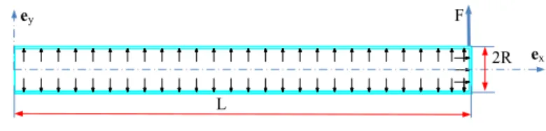
The results obtained in the previous Section will now be applied to the bending of a cantilever pressurized membrane tube. In the pre-stressed reference configuration, the tube is subjected to an internal pressure p, its geometry is a closed axisymmetric cylindrical tube, of length L, radius R and thickness H, see Figure 8. The tube is clamped at the end X = 0 and free at the other end X = L. After the pressurization, a force Feyis applied at the end X = L.
ey
2R L
ex F
Figure 8: Cantilever pressurized membrane tube subjected to a bending loading
From Equations (42)1and (43)1−2, one gets N0(X ) = P. The static boundary
con-ditions in terms of V andθresult from (43)3−6:
(P + kGℓtS0)(V,X(L)−θ(L)) = F θ,X(L) = 0 (44)
Solving (42)2−3and (44) under the kinematic boundary conditions V (0) =θ(0) = 0
leads to the deflection and the rotation:
V (X ) = F (Eℓ+ P S0 )I0 (LX 2 2 − X3 6 ) + FX P + kGℓtS0 θ(X ) = F (Eℓ+ P S0 )I0 (LX−X 2 2 ) (45)
These relations clearly show the significant role of the internal pressure p – via the pressure resultant P≡ pπR2– in the bending and shear stiffnesses of the beam. Equations (45) slightly differ from those given in [12]. With our notations, the modulus
∅E¯ℓ= ∅Eℓ
1−∅νℓt∅νtℓ
in [12] is replaced here by Eℓand the term
1 2k
∅G
ℓtS0in [12] is
Influence of the internal pressure on the stiffness moduli
Relations (45) show that the internal pressure modifies the shear stiffness kGℓtS0, as
is the case in Fichter’s formulas [6] for the isotropic beam. The pressure also modifies the bending stiffness EℓI0, which extends the result proven in [10] for the isotropic
beam again. The formulation of the orthotropic beam may seem elaborate, but the final result is rather intuitive: the transition from the isotropic to the orthotropic case amounts to replacing the Young’s modulus E by Eℓand the shear modulus G by Gℓt.
In order to quantify the impact of the pressure on the stiffness moduli, let us recast the bending stiffness as
(Eℓ+P S0 )I0= (Eℓ+ pπR 2 2πRH)πR 3H = (E ℓH + pR 2 )πR 3 (46)
Thus, the change in the Young’s modulus due to the pressure is expressed by the correction term pR/2. Likewise, the shear stiffness can be rewritten as
P + kGℓtS0= pπR2+ kGℓt2πRH = 2πRk(GℓtH + pR
2k) (47)
which shows that the change in the shear modulus GℓtH is equal to pR, by taking k = 0.5 (value for thin tubes).
Consider again the two beams corresponding to two different rolling directions of the orthotropic membrane, denoted Orientation 1 and Orientation 2, with the numerical data given in Table 1. By using the values in Table 2, one can compute the change of the stiffness moduli due to the internal pressure. Table 3 displays the results obtained with pressure p equal to 300kPa.
The shear modulus is more affected by the internal pressure, since it is smaller than the Young’s modulus (as is usually the case with fabrics). However, it is found that the change in the Young’s modulus - with and without the pressure correction term - is not always negligible, it can be either small (3%) or significant (9%). The herein proposed beam theory enables one to precisely compute the stiffness change due to the pressure and decide when some term or other can be neglected.
Influence of the internal pressure on the deflections
Let us now examine the influence of the internal pressure on the beam deflections. For the cantilever beam of interest, the tip deflection V (L) given by (45) can be split