Probabilistic dynamic analyses of a soil-structure system subjected to a stochastic earthquake Ground-Motion

HAL Id: hal-01008681

https://hal.archives-ouvertes.fr/hal-01008681

Submitted on 30 Oct 2019

HAL is a multi-disciplinary open access

archive for the deposit and dissemination of sci-entific research documents, whether they are pub-lished or not. The documents may come from teaching and research institutions in France or abroad, or from public or private research centers.

L’archive ouverte pluridisciplinaire HAL, est destinée au dépôt et à la diffusion de documents scientifiques de niveau recherche, publiés ou non, émanant des établissements d’enseignement et de recherche français ou étrangers, des laboratoires publics ou privés.

Probabilistic dynamic analyses of a soil-structure system

subjected to a stochastic earthquake Ground-Motion

Tamara Al-Bittar, Panagiotis Kotronis, Stéphane Grange, Abdul-Hamid

Soubra

To cite this version:

Tamara Al-Bittar, Panagiotis Kotronis, Stéphane Grange, Abdul-Hamid Soubra. Probabilistic dy-namic analyses of a soil-structure system subjected to a stochastic earthquake Ground-Motion. WCCM 2012, 10th World congress on computational mechanics, Jul 2012, São Paulo, Brazil. �10.5151/meceng-wccm2012-18591�. �hal-01008681�

PROBABILISTIC DYNAMIC ANALYSIS OF A SOIL-STRUCTURE SYSTEM SUBJECTED TO A STOCHASTIC EARTHQUAKE GROUND-MOTION

Al-Bittar T1_{, Kotronis P}2_{, Grange S}3_{, Soubra A-H}4

1_{PhD student, LUNAM Université, University of Nantes, Bd. de l’université, BP 152, 44603 Saint-Nazaire cedex, France,}

E-mail: Tamara.Al-Bittar@univ-nantes.fr

2_{Professor, LUNAM Université, Ecole Centrale de Nantes, GeM (Research Institute of Civil Engineering and Mechanics)}

CNRS UMR 6183 1 rue de la Noë, BP 92101, 44321, Nantes, cedex 3, France, E-mail: Panagiotis.Kotronis@ec-nantes.fr

3_{Associate Prof., UJF-Grenoble 1, G-INP, CNRS UMR 5521, Lab 3SR, Grenoble F-38041, France; E-mail:}

stephane.grange@ujf-grenoble.fr

4_{Professor, LUNAM Université, University of Nantes, Bd. de l’université, BP 152, 44603 Saint-Nazaire cedex, France,}

E-mail: Abed.Soubra@univ-nantes.fr

Abstract. In this paper, a probabilistic dynamic analysis of a five-storey building subjected to a

stochastic earthquake Ground-Motion (GM) is presented. The entire soil-structure system is considered in the analysis. The stochastic GM time-histories are based on a real recorded time history. The probabilistic dynamic analysis is performed using the classical Monte Carlo Simulation (MCS) methodology. As is well known, this method requires a great number of calls of the deterministic model. To overcome the inconvenience of the time cost, a simple deterministic model based on the "macro-element" concept is used. The main advantage of the macro-element is that the time cost for a single deterministic calculation is relatively small and thus, this model is suitable for the probabilistic dynamic analysis. The simulation of the stochastic GM time-histories is done using a fully non-stationary stochastic model in both the time and the frequency domains. This model employs filtering of a discretized white-noise process. Non-stationarity is achieved by modulating the intensity and by varying the filter properties in time. As for the probabilistic analysis, a large number of samples (say 100,000) of the stochastic GM time-histories is generated using Monte Carlo technique. For each sample, a dynamic calculation using the macro-element is performed and the following responses are retained for the probabilistic analysis: (i) the maximum horizontal displacement at the top of the building, (ii) the three maximum displacements of the footing centre, and finally (iii) the three maximum reaction forces at the contact of the soil and the footing. These results are used to compute the statistical moments of the different system responses together with the probability of exceeding of predefined thresholds for these responses.

Keywords: dynamic analysis, stochastic ground-motion, macro-element.

1. INTRODUCTION

Different experimental results and in-situ observations after strong earthquakes [8, 13 among others] have shown that the soil plasticity and the uplift of the foundation (called hereafter the soil and soil-structure interface nonlinearities) often result in structural isolation. This leads to a reduction in the forces and moments that may develop in the structure. The maximum values of the stresses in the structure decrease because of the large energy dissipation in the soil and soil-structure interface. Blucher Mechanical Engineering Proceedings

May 2014, vol. 1 , num. 1

Notice however that an important increase in the displacement occurs at the top of the structure. This is due to (i) the inertial effects of the structure and (ii) the soil and soil-structure non-linearities.

In order to study a soil-structure interaction (SSI) problem, three methods can be found in literature [11]: (i) The superposition method which subdivides the complex SSI problem into simpler problems (kinematics interaction and inertial interaction [9]), this method being valid only for linear problems, (ii) The direct methods that use a classical finite element approach [12], but these methods require good knowledge of the constitutive laws and are computationally-expensive and (iii) The hybrid methods that are a combination of the two previous methods and therefore they are more attractive because of their computational cost. The macro-element approach belongs to this last category. The macro-element concept developed by [10] consists in condensing the soil (material) and interface (geometric) nonlinearities into a representative point (the centre of the foundation) and it works with generalized variables (forces and displacements). It thus allows the simulation of the behaviour of shallow foundations in a simplified way. Several 2D macroelements exist in literature [2, 3, 10]. The 2D macro-element developed in [4] is adequate for static, cyclic and dynamic loadings (e.g. earthquake) and it considers both the plasticity of the soil and the uplift of the foundation. Grange et al. [6] have extended the macro-element of [4]. Their macro-element can simulate the 3D behaviour of foundations having different shapes (circular, rectangular and strip). This recent version of the macro-element is adopted in this paper to perform the probabilistic dynamic analysis. The main reason for which the macro-element concept is chosen to perform the probabilistic analysis is that the time cost for a single deterministic calculation is relatively small. Thus, this model is suitable for the probabilistic analysis which requires a great number of calls of the deterministic model.

In this paper, a probabilistic dynamic analysis of a five-storey building founded on a two rigid rectangular footings and subjected to a stochastic earthquake Ground-Motion (GM) is presented. The entire soil-structure system is considered and the soil and soil-footing interface are modelled using the macro-element. The stochastic GM time-histories are based on a real recorded time history. The probabilistic dynamic analysis is performed using the classical Monte Carlo Simulation (MCS) methodology. The paper is organized as follows: The next two sections aim at briefly presenting (i) the method used to generate the stochastic synthetic accelerograms based on a real target one, and (ii) the mathematical description of the macro-element. They are followed by the presentation of the numerical results. The paper ends with a conclusion.

2. GENERATION OF STOCHASTIC GROUND MOTION ACCELEROGRAMS

In this paper, the method proposed by [15] was used to generate stochastic synthetic acceleration time histories from a target accelerogram which is a real recorded acceleration time history. This method consists in fitting a parameterized stochastic model that is based on a modulated, filtered white-noise process to a recorded ground motion. The parameterized stochastic model in its continuous form is defined as:

[

]

1 ( ) ( , ) , ( ) ( ) ( ) t i h x t q t h t w d t

α

τ λ τ

τ τ

σ

−∞      = _{ } − _    

∫

 (1)

In this expression,

q t

( , )

α

is a deterministic, positive, time-modulating function with parameters αi controlling its shape and intensity;

w

( )

τ

is a white-noise process; the integral inside the brackets is a

filtered white-noise process with

h t

[

−

τ λ τ

, ( )

]

denoting the Impulse-Response Function (IRF) of the filter where

λ τ

( )

is a time-varying vector of parameters; and 2_{( )} t 2

[

_{, ( )}

]

h t h t d

σ τ λτ τ

−∞

=

∫

− is the

variance of the integral process. Because of the normalization by

σ

h

( )

t

, the process inside the

brackets has unit variance. As a result,

q t

( ,

α

i

)

equals the standard deviation of the resulting process

x(t). It should be noticed that the modulating function

q t

( ,

α

i

)

completely defines the temporal

characteristics of the process, whereas the form of the filter IRF and its time-varying parameters define the spectral characteristics of the process. In this study, a ‘Gamma’ modulating function is used as follows:

2 1

1 3

( ,

i

)

exp(

)

q t

α

=

α

t

α −

−

α

t

(2)

In this equation,

α

i

=

( ,

α α α

1 2

,

3

)

where

(

α α >

1

,

3

)

0

, and

α >

2

1

. Of the three parameters, α1 controls the intensity of the process; α2 controls the shape of the modulating function and α3 controls the duration of the motion. These parameters are related to three physically based parameters

5 95

( ,

I D

a −

,

t

mid

)

which describe the real recorded GM in the time domain; where

I

a is the Arias

Intensity (AI) and D5−95 represents the effective duration of the motion. D5−95 is defined as the time interval between the instants at which the 5% and 95% of the expected AI are reached respectively. Finally, tmid is the time at the middle of the strong-shaking phase. It is selected as the time at which 45% of the expected AI is reached. The relationship between

α

i

=

( ,

α α α

1 2

,

3

)

and

( ,

I D

a 5 95−

,

t

mid

)

are given in details in [15] and are not presented herein.

For the filter IRF, we select a form that corresponds to the pseudo-acceleration response of a single-degree-of-freedom linear oscillator:

[

]

2 2 ( ) , ( ) exp ( ) ( )( ) sin ( ) 1 ( )( ) 1 ( ) 0 otherwise f f f f f f h t τ λ τ ω τ ζ τ ω τ τt ω τ ζ τ τ t τ t ζ τ     − = − _ − × _{ }− − ≤ _ − = (3) where

λ τ

( ) (

=

ω τ ζ τ

f

( ),

f

( ))

is the set of time-varying parameters of the IRF with

ω τ

f

( )

denoting

the frequency of the filter and

ζ τ

f

( )

denoting its damping ratio. These two parameters are related to

the two physical parameters that describe the recorded GM in the frequency domain and which are respectively the predominant frequency and the bandwidth of the GM. For more details about the identification procedure between the recorded GM and the stochastic model described previously, the reader may refer to [14-15].

3. MATHEMATICAL DESCRIPTION OF THE MACRO-ELEMENT

The purpose of this section is to describe a theoretical model based on strain hardening plasticity theory which is capable of describing the behavior of a shallow footing when it is subjected to all possible combinations of vertical, horizontal and moment loading using the macro-element. In the framework of the macro-element theory, any load or deformation path can be applied to the footing and the corresponding unknowns (deformations or loads) can be calculated. The foundation is assumed to be rigid and the nonlinearities of the soil and interface are assumed to be condensed in a representative point which is the footing centre. Within that framework, it is suggested to work with generalized (global) variables: (i) the force resultants, i.e. the vertical force V, the horizontal forces Hx,

Hy, and the moments Mx, My and (ii) the corresponding displacements; i.e. the vertical displacement uz, the horizontal displacements ux and uy, and the rotations θx and θy. The torque moment (Mz) and the corresponding displacement are not taken into account in the present analysis. The three-dimensional SSI macro-element takes into account three different mechanisms: the soil elasticity, the possible soil plasticity and the possible uplift of the foundation. The total displacement can thus be considered as a sum of three components related to the elastic and plastic behavior of the soil and the uplift behavior of the foundation. These three different mechanisms and their mathematical development are extensively presented in [3, 6, 7] and are briefly described herein.

3.1. Elastic behaviour

The elastic constitutive model can be written as

F

r

=

K

el

(

u u

r r

−

pl

)

where

(

'

_z

'

_x

'

_y

'

_y

'

_x

)

u

r

=

u

u

θ

u

θ

and

F

r

=

(

V

'

H

'

_x

M

'

_y

H

'

_y

M

'

_x

)

are the vectors that represent the dimensionless generalized displacements and forces and Kel _{is the elastic stiffness matrix}

[6].

3.2. Plastic behaviour - failure criterion and loading surface

The loading surface used was initially developed in [3] to describe the behaviour of a 2D shallow foundation. The extension of this loading surface to cover the case of a 3D shallow foundation is a five-dimensional surface. It is given as follows:

(

)

(

)

(

)

(

)

2 2 2 2

'

'

( , , , )

'

'

'

'

'

_'

1 0

'

'

'

'

y x c _c d _e f y x d f c e

M

H

f F

aV

V

bV

V

H

_M

aV

V

bV

V

α

β

τ ρ γ

ρ

ρ

ρ

γ

ρ

γ

δ

η

ρ

ρ

ρ

γ

ρ

γ

















≡

_

−

_

+

_

−

_

−

−

























+

_

−

_

+

_

−

_

− =

−

−









r

(4)

The coefficients a and b define the size of the surface in the plane (H'-M'), and the coefficients c, d, e and f define the parabolic shape of the surface in the planes (V'-M') and (V'-H'). Theses parameters can be obtained by fitting this equation to experimental results. On the other hand, the vector

(

, , ,

)

τ

r

=

α β δ η

is the kinematics hardening vector. It is composed of 4 kinematics hardening

variables and

ρ

is the isotropic hardening variable. The variable γ is chosen to parameterize the second intersection point of the loading surface with the V' axis and its evolution in the V' axis (the other point is the origin of the space). The evolution of the hardening variables is obtained by considering experimental results and numerical simulations [3]. Notice finally that the failure criterion is given by equation (4) with

(

α β δ η ρ γ =, , , , ,

) (

0, 0, 0, 0,1,1

)

.

3.3. Uplift behaviour - failure criterion and loading surface

The uplift behaviour is not influenced by the horizontal forces. For the uplift mechanism, the failure criterion is given by [6] as follows:

(

)

2 2 ' 2 1

'

'

V

AV

0

f

M

e

q

q

− ∞





≡

−

_

+

_

=





(5)

where A is a parameter of the constitutive model and (q1, q2) is a couple of integers that takes into account the shape of the foundation. As for the loading surface, its evolution is more complicated than for a classical plasticity model. Thus, it is not presented herein. For more details, the reader may refer to [6]. The uplift mechanism is coupled with the plasticity mechanism by using the classical multi-mechanism approach.

4. PROBABILISTIC NUMERICAL RESULTS

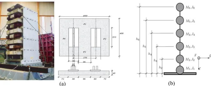
The aim of this section is to present the probabilistic numerical results. It should be remembered here that the dynamic analysis involves a five-storey building subjected to a stochastic earthquake Ground-Motion (GM). The CAMUS IV structure [1] is chosen in this study. This structure is a 1/3 scaled mock-up. It is composed of (i) two parallel five-floor reinforced concrete walls without opening and (ii) six square floors that link these walls (Figure 1(a)). The entire structure rests on two rectangular footings of 0.8mx2.1m (Figure 1(a)). The total height of the model is 5.1 m and the total mass is estimated to be equal to 36 tons. The wall of a given floor is 4m long, 1.70m high and 6 cm thick [1]. The building and the footings rest on a high density sand. The container which contains the sand has a horizontal cross-section of 4.6mx4.6m and a depth of 4m.

(a)

(b)

Figure 1. The five-storey building: (a) The CAMUS IV real model, and (b) the simplified numerical lumped mass system

For the numerical calculations, the CAMUS IV five-storey building is modelled using a simple lumped mass system (Figure 1(b)). In this system, the building is simulated using beam elements and concentrated masses. Each storey i is reduced to a single mass Mi that has an inertia equal to Ji. The values of the masses and the corresponding inertias for the different stories are given in Table 1. The material behaviour of the beams is considered linear elastic. The soil-foundation system is modelled using the macro-element which has two superposed nodes. The first node is considered fixed and the

second node is connected to the structure. The dynamic loading is applied to that first node. For the used height density sand, [7] have identified the different parameters of the macro-element by fitting the model to the experimental results given by [5]. These parameters are presented in Table 2 where qmax is the ultimate bearing capacity of the rectangular footing, a, b, c, d, e and f are the coefficients that appear in Equation (4), κ and ξ are parameters of the flow rule, and finally a1, a2, a3, a4 and a5 are parameters used to calculate the variable γ as may be seen in [5].

Table 1. Parameters used to model the five-storey building Height hi [m] (see Figure 1) Mass [Kg] Inertia [Kg.m2_] h1=0.1 M1=4786 J1=1600 h2=1.4 M2=6825 J2=3202 h3=2.3 M3=6825 J3=3202 h4=3.2 M4=6825 J4=3202 h5=4.1 M5=6825 J5=3202 h6=5 M6=6388 J6=3124

Table 2. Parameters used to model the soil-foundation (macro-element) Elastic parameters el

K

_θθ=52MNm/rad el hh

K

=105MN/m el zz

K

=120MN/m Plastic parameters qmax=0.58MPa κ=1 a=0.93 ξ=1 b=0.8 a1=1 c=1 a2=1 d=1 a3=1 e=1 a4=1 f=1 a5=1

In the following sections, some typical stochastic synthetic acceleration time histories used to perform the probabilistic analysis are presented. The probabilistic results are then presented and discussed.

4.1. Realizations of the stochastic synthetic acceleration time histories

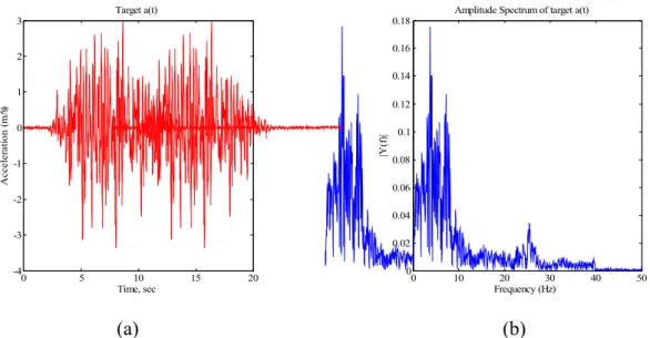
The target acceleration time history used to generate stochastic synthetic acceleration time histories is the Nice synthetic accelerogram shown in Figure 2(a). This signal is representative of the French design elastic response spectrum. It has a maximum acceleration equal to 0.33g and its Fourier amplitude spectrum is given in Figure 2 (b). The target acceleration time history shown in Figure 2 is used to identify the parameters of the stochastic model given in Equation (1). Once these parameters are calculated using the target accelerogram, realizations of the stochastic synthetic acceleration time histories can be performed by generating for each simulation a new white noise which is a series of standard normal random variables.

0 10 20 30 40 50 0 0.02 0.04 0.06 0.08 0.1 0.12 0.14 0.16

0.18 Amplitude Spectrum of target a(t)

Frequency (Hz) |Y (f )| 0 5 10 15 20 -4 -3 -2 -1 0 1 2 3 Target a(t) Time, sec A cc el er at io n (m /s 2)

(a)

0 10 20 30 40 50 0 0.02 0.04 0.06 0.08 0.1 0.12 0.14 0.16

0.18 Amplitude Spectrum of target a(t)

Frequency (Hz) |Y (f )| 0 5 10 15 20 -4 -3 -2 -1 0 1 2 3 Target a(t) Time, sec A cc ele ra ti on ( m /s 2)

(b)

Figure 2. (a) The target acceleration time history, and (b) its corresponding Fourier amplitude spectrum

Figure 3 presents five realizations of the stochastic synthetic acceleration time histories. This figure shows that the different simulated acceleration time histories have different maximum accelerations which will induce different dynamic responses. The aim of the next two subsections is to present respectively (i) the probability density function PDF of the dynamic responses obtained using 100,000 stochastic synthetic acceleration time histories, and (ii) the fragility curves corresponding to three different damage levels.

0 5 10 15 20 -5 -4 -3 -2 -1 0 1 2 3 4 Time, sec A cc el er at io n (m /s 2)

Real earthquake (Nice 0.33g) Simulation 1 Simulation 2 Simulation 3 Simulation 4 Simulation 5

(a)

0 10 20 30 40 50 0 0.02 0.04 0.06 0.08 0.1 0.12 0.14 0.16 0.18 Frequency (Hz) |Y (f )|

Real earthquake (Nice 0.33g) Simulation 1 Simulation 2 Simulation 3 Simulation 4 Simulation 5

(b)

Figure 3. (a) Target and five simulated acceleration time-histories, and (b) their corresponding Fourier amplitude spectrum

4.2. Statistical moments of the dynamic responses

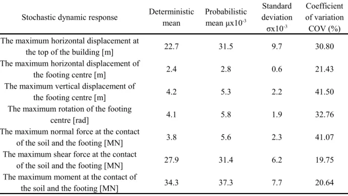
Table 3 presents the two first statistical moments (i.e. the probabilistic mean and the standard deviation) together with the deterministic mean values for the following dynamic responses: (i) the maximum horizontal displacement at the top of the building, (ii) the three maximum displacements of the footing centre, and finally (iii) the force resultants (Vmax, Nmax, Mmax) at the contact of the soil and the footing. This table shows that the probabilistic mean value of the maximum horizontal

displacement at the top of the building is almost 10 times larger that the one obtained at the footing centre. On the other hand, large values of the coefficient of variation COV are obtained for the

different output parameters (19.75<COV<41.5). From a probabilistic point of view, large values of the coefficient of variation indicate that the responses are spread out over a large range of values. This is critical since in this case the mean values of these responses are not representative and can not be considered as reliable data for design procedure. For some output parameters (such as the maximum displacement at the top of the building and the maximum moment at the bottom), this phenomenon is amplified by the fact that the probabilistic mean value is significantly larger than the deterministic one.

Table 3. Effect of stochastic Ground-Motion on the statistical moments (μ, σ) of the seven dynamic responses

Stochastic dynamic response Deterministic mean Probabilistic mean μx10-3 Standard deviation σx10-3 Coefficient of variation COV (%) The maximum horizontal displacement at

the top of the building [m] 22.7 31.5 9.7 30.80

The maximum horizontal displacement of

the footing centre [m] 2.4 2.8 0.6 21.43

The maximum vertical displacement of

the footing centre [m] 4.2 5.3 2.2 41.50

The maximum rotation of the footing

centre [rad] 4.1 5.8 1.9 32.76

The maximum normal force at the contact

of the soil and the footing [MN] 3.8 5.6 2.3 41.07 The maximum shear force at the contact

of the soil and the footing [MN] 27.9 31.4 6.2 19.75 The maximum moment at the contact of

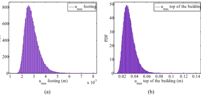
the soil and the footing [MN] 34.3 37.3 7.7 20.64 Figure 4 presents the PDF of the maximum horizontal displacement at the footing centre and that of the maximum horizontal displacement at the top of the building. This figure shows that the PDF of the maximum horizontal displacement at the top is more spread out and thus more critical.

1 2 3 4 5 6 7 8 x 10-3 0 200 400 600 800 u_max footing (m) PD F u_max footing

(a)

0.02 0.04 0.06 0.08 0.1 0.12 0.14 0 10 20 30 40 50

u_max top of the building (m)

PDF

u_max top of the building

(b)

Figure 4. PDF of the maximum horizontal displacement (a) at the centre of the footing, and (b) at the top of the building

4.3. Fragility curves

The probability that a certain level of damage (tolerable maximum horizontal displacement) will be exceeded at a specified ground motion level can be expressed in the form of fragility curves. The fragility curves can be performed since the stochastic ground motions create variability in the PGA (0.2g<PGA<0.7g). In this section, fragility curves for the maximum horizontal displacement at the top of the building and for the maximum moment at the contact of the soil and the footing are computed. Figure 6(a) presents three fragility curves corresponding to the maximum horizontal displacement at the top of the building for three levels of damage [(i) minor damage for which umax=0.06m, (ii) medium damage for which umax=0.04m and (iii) major damage for which umax=0.01m]. On the other hand, Figure 6(b) presents three fragility curves corresponding the maximum moment at the contact of the soil and the footing for three levels of damage [(i) minor damage for which Mmax=0.06MNm, (ii) medium damage for which Mmax=0.04MNm and (iii) major damage for which Mmax=0.01MNm]. For the probabilistic analysis, these figures allow one to determine the probability of exceeding a tolerable value of the dynamic response corresponding to a given value of the peak ground acceleration (PGA) for a prescribed damage level.

0.1 0.2 0.3 0.4 0.5 0.6 0.7 0.8 0 0.1 0.2 0.3 0.4 0.5 0.6 0.7 0.8 0.9 1 PG A(g) Pr ob ab ili ty o f f ai lu re

M ajor level of dam age (u_max=0.01m )

M edium level of dam age (u_max= 0.04m )

M inor level of dam age (u_max= 0.06m )

(a)

0.1 0.2 0.3 0.4 0.5 0.6 0.7 0.8 0 0.1 0.2 0.3 0.4 0.5 0.6 0.7 0.8 0.9 1 P G A(g) Pr ob ab ili ty o f f ai lu re

M ajor level of dam age (M_max=0.01M N m ) M edium level of damage (M_max=0.04M N m ) M inor level of dam age (M_max=0.06M N m )

(b)

Figure 6. Fragility curves for different level of damage (a) maximum moment at the contact of the soil and footing, and (b) maximum horizontal displacement at the top of the building

5. CONCLUSION

In this paper, a probabilistic dynamic analysis of a five-storey building founded on two rigid

rectangular footings and subjected to a stochastic earthquake Ground-Motion (GM) is presented. The entire soil-structure system is considered in the analysis in which the soil and soil-footing interface are modelled by a macro-element. The stochastic GM time-histories are based on a real recorded time history. The probabilistic dynamic analyses are performed using the classical Monte Carlo Simulation (MCS) methodology. The probabilistic results have shown that (i) the probabilistic mean value of the maximum horizontal displacement at the top of the building is almost 10 times larger that the one obtained at the footing centre; (ii) large values of the coefficient of variation are obtained for the maximum horizontal displacement at the top of the building and for the maximum moment at the contact of the soil and the footing; and finally (iii) stochastic ground motion time histories create variability in the PGA which allows one to perform fragility curves for the different dynamic responses.

REFERENCES

[1] CAMUS International Benchmark. Mock-up and loading characteristics, specifications for the participants report, Report I, CEA and GEO 1997.

[2] Cassidy MJ, Byrne BW, Houlsby GT. Modelling the behaviour of circular footings under combined loading on loose carbonate sand. Géotechnique 2002; 52(10):705–712.

[3] Crémer C, Pecker A, Davenne L. Cyclic macro-element for soil–structure interaction: material and geometrical non-linearities. International Journal for Numerical and Analytical Methods in

[4] Crémer C, Pecker A, Davenne L. Modelling of nonlinear dynamic behaviour of a shallow strip foundation with macro-element. Journal of Earthquake Engineering 2002; 6(2):175–211.

[5]

Grange, S. Risque sismique: stratégie de modélisation pour simuler la réponse des

structures en béton et leurs interactions avec le sol. PhD Thesis INPG 2008

[6] Grange S, Kotronis P, and Mazars, J. A macro-element to simulate 3D soil–structure interaction considering plasticity and uplift. International Journal of Solids and Structures 46 (2009) 3651–3663 [7] Grange S, Kotronis P, and Mazars, J A macro-element to simulate dynamic Soil-Structure Interaction. Engineering Structures 31 (2009) 3034–3046

[8] Housner GW. The behaviour of inverted pendulum structures during earthquakes. Bulletin of the Seismological Society of America 1963; 53(2):403–417.

[9] Kausel E, Whitman A, Murray J, Elsabee F. The spring method for embedded foundations. Nuclear Engineering and Design 1978; 48:377–392.

[10] Nova R, Montrasio L. Settlements of shallow foundations on sand. Géotechnique 1991; 41(2):243 256.

[11] Pecker A. Dynamique des Sols. Presse, ENPC: Paris, France, 1984.

[12] Prévost JH. DYNAFLOW. A finite element analysis program for static and transient response of linear and nonlinear two and three dimensional systems. User Manual, Department of Civil

Engineering, Princeton University, 1999.

[13] Psycharis IN. Dynamic behavior of rocking structures allowed to uplift. Journal of Earth Engineering and Structural Dynamics 1983; 11:57–76, 501–521.

[14] Rezaeian S, and Der Kiureghian A. A stochastic ground motion model with separable temporal and spectral nonstationarity. Earthquake Engineering and structural dynamics 2008; 37: 1565–1584. [15] Rezaeian S, and Der Kiureghian A. Simulation of synthetic ground motions for specified earthquake and site characteristics. Earthquake Engineering and structural dynamics 2010; 39: 1155– 1180.