HAL Id: hal-01163826
https://hal-mines-albi.archives-ouvertes.fr/hal-01163826
Submitted on 15 Jun 2015
HAL is a multi-disciplinary open access
archive for the deposit and dissemination of
sci-entific research documents, whether they are
pub-lished or not. The documents may come from
L’archive ouverte pluridisciplinaire HAL, est
destinée au dépôt et à la diffusion de documents
scientifiques de niveau recherche, publiés ou non,
émanant des établissements d’enseignement et de
CARLO DIRECT MODEL
Olivier Farges, Jean-Jacques Bézian, Mouna El-Hafi, Olivier Fudym, Hélène
Bru
To cite this version:
Olivier Farges, Jean-Jacques Bézian, Mouna El-Hafi, Olivier Fudym, Hélène Bru.
PARTICLE
SWARM OPTIMIZATION OF SOLAR CENTRAL RECEIVER SYSTEMS FROM A MONTE
CARLO DIRECT MODEL. IPDO 2013 : 4th Inverse problems, design and optimization symposium,
Jun 2013, Albi, France. �hal-01163826�
PARTICLE SWARM OPTIMIZATION OF SOLAR CENTRAL RECEIVER
SYSTEMS FROM A MONTE CARLO DIRECT MODEL
Olivier Fargesa,b, Jean-Jacques Béziana, Mouna El Hafia, Olivier Fudyma, and Hélène Brub aCentre RAPSODEE, UMR CNRS 5302, École des Mines d’Albi-Carmaux, Université de Toulouse, 81013
Albi Cedex 09, France, olivier.farges@mines-albi.fr, jean-jacques.bezian@mines-albi.fr, mouna.elhafi@mines-albi.fr, olivier.fudym@mines-albi.fr
bTotal New Energies, R&D - Concentrated Solar Technologies, Tour Michelet ,Paris La Défense, France,
helene.bru@total.com
Abstract
Considering the investment needed to build a solar concentrating facility, the performance of such an installation has to be maximized. This is the reason why the preliminary design step is one of the most important stage of the project process. This paper presents an optimization approach coupling a Particle Swarm Optimization algorithm with a Monte Carlo algorithm applied to the design of Central Receiver Solar systems. After the validation of the direct model from experimental data, several PSO algorithms are tested to pick out efficient parameters.
Nomenclature Roman symbols
B Blocking performance in % CRS Central Receiver System
c1 Attraction parameter for individual
behav-ior of the particle
c2 Attraction parameter for social behavior of
the particle
DN I Direct normal irradiance in W · m−2 d(r(x∗)) Distance to the maximum obtained cost
reduction
E Yearly average energy in kWh f Target function
fc Threshold for the number of failures during
GCPSO run
gk Global best position of the swarm after k
iterations
GCP SO Guaranteed Convergence Particle Swarm Optimizer
H Heliostats surface (the exponent + indicate the active side)
H The Heaviside step function Ht Height of the CRS Tower in m
kmax Number of iterations performed during
PSO run
n1 Ideal normal at x1
nh Effective normal at x1around the ideal
nor-mal n1
Nm Number of mirrors constituting heliostat
pki Particle i best position after k iterations P SO Particle Swarm Optimizer
r1 Random number r1∼ U (0, 1)
r2 Random number r2∼ U (0, 1)
r(x∗) Normalized cost reduction
Sh Shadowing performance in % Sp Spillage performance in %
sc Threshold for the number of successes
dur-ing GCPSO run
Sm Size of mirrors constituting heliostats in m
SH+ Area of mirror in m2
T Target (the exponent + indicate the active side)
t Time in s
T M Y Typical Meteorological Year
vki Current velocity of the i particle at the k it-eration
ˆ
w Monte Carlo weight w Inertia weight
wmax Maximum value of the weight inertia
wmin Minimum value of the weight inertia
xk
i Current position of the i particle at the k
it-eration
x∗ Best particle for each test case ˆ
x Best particle among all test cases yj Point in the geometry
Greek symbols
η Hour in h: min: s γ Day of the year
ΩS Solar cone in sr
ω1 Direction after reflection in rad
ωS Direction inside the solar cone in rad
ρk Scaling factor applied in GCPSO τ Index of the swarm best particle
Introduction
A Central Receiver System (CRS) is a complex set composed of several different subsystems including heliostat field, tower, receiver, heat transport system, power conversion system, plant control, optionally a thermal energy storage, etc. To generate heat further used to produce electricity, synthetize solar fuels or supply an industrial process, the solar radiation is first reflected and concentrated by an heliostat field onto a receiver located at the top of a tower. A large proportion of the cost of a CRS plant is devoted to the heliostat field (∼ 50%) according to [1]. In consequence, it’s necessary to pay special attention to this item during the preliminary design step of any CRS. Since the 70’s, several studies have been dedicated to the optimization of central receiver systems and most of them specifically on heliostat fields. Among the most recent developments, we can quote [2], [3], [4] and [5]. Each of these studies deal with a specific set of parameters (either those describing the layout of the heliostat field, or the heliostat geometrie and size, or the height of the tower...). Evaluation of performance is often based on optical efficiency estimation. This parameter agregates reflection efficiency, cosine efficiency, interception efficiency, blocking and shadow-ing efficiency and transmission efficiency. These efficiency values are usually obtained from simplified mathematical models or ray tracing simulations with the constraint accomplishing optimization step in a reasonable computational time.
1. Model descrition
In this paper, we present a new approach using a direct model based on Monte Carlo methods that is further combined with a stochastic optimization algorithm. Achievement of an optimization task requires an efficient direct model related to the target function used during optimization process.
1.1 Modeling the annual energy collected
In the present case, the direct model simulates a central receiver system. It estimates the annual perfor-mance of a CRS by evaluating the annual energy collected at the receiver and the optical efficiency. From a radiative point of view, the evaluated quantity is the solar energy E at the entrance of a receiver after concentration by the heliostat field. In order to evaluate E, the direct model has to track positions of the sun of a typical year cycle. Doing so, all the geometry is dynamic, i.e. heliostats are redirected according to sun position. The quantity of interest is linked to the solar radiation data for a chosen area, coming from Typical Meteorological Year (TMY) file. Being a function of the Direct Normal Irradiance (DNI), the annual energy’s estimation requires a DNI value for each instant. This value is obtained from linear interpolation between consecutive TMY data which are sampled every hour.
1.2 Monte Carlo algorithm
Monte Carlo method, due to its integral formulation, allows a better convergence of the algorithm. Sev-eral CSP algorithms are developped in accordance with this principle [6] (central receiver systems, Fresnel linear collectors, fluidized bed receiver, enclosed solar photobioreactor). An overview of the specific Monte Carlo algorithm, dealing with the sun’s positions in the sky, is presented on Fig. 1. This algorithm sam-ples some dates from a uniform distribution, then locations on the heliostat field where sun rays are first reflected, after which it follows rays behavior in the CRS, ie computes reflections until each ray hits the final receiver :
(1) A position of the sun is uniformly sampled over the year with a day γ and an hour η
(2) A location y1is uniformly sampled on the reflective surface of the whole heliostat field H+of surface
SH+
(3) A direction ωsis uniformly sampled within the solar cone C of angular radius Ωs. In order to identify
shadowing effects, the location y0 is defined as the first intersection with a solid surface of the ray
starting at y1in the direction ωs:
(a) If y0 belongs to heliostat surface H or to the receiver T , a shadowing effect appears and the
algorithm restarts at (1) with Monte Carlo weight ˆwout = 0 ;
(b) If y0doesn’t exist, the reflected direction ω1is sampled so as to represent reflection and pointing
imperfections. The location y2 defined as the first intersection of the ray starting at y1 in the
direction ω1is checked :
(i) If y2belongs to something else than the receiver T , there is a blocking effect and the
algo-rithm restarts at (1) with Monte Carlo weight ˆwout= 0 ;
(ii) If y2doesn’t exist, there is a spillage effect and the algorithm restarts at (1) with Monte Carlo
weight ˆwout= 0 ;
(iii) If y2belongs to the receiver T , the algorithm restart at (1) with Monte Carlo weight ˆwin=
DN I × (ωs· nh) × SH+ where nhis the effective normal at y1around the ideal normal
vector n1;
This algorithm is equivalent to the integral formulation presented in Eq. (1).
E = Z 365 1 pΓ(γ)dγ Z 12P.M. 0A.M. pH(η)dη Z H+ pY1(y1)dy Z ΩS pΩS(ωS)dωS× ( H(y0∈ (H ∪ T )) ˆwout +H(y0∈ (H ∪ T ) ×/ Z DNh
pNh(nh|ωS; p)dnh{H(y2∈ T ) ˆ/ wout+ H(y2∈ T ) ˆwin}
)
(1)
1.3 A specific computing framework
The direct model is implemented in the numerical framework EDStaR. This tool yields the practical implementation of a Monte Carlo algorithm for the radiative heat transfer model, making use of an integral formulation, and takes in consideration zero-variance approaches and sensitivity estimation as presented by [7] and [8]. Taking advantage of advanced rendering techniques developped by the computer graphics community, it can manage complex geometries with the use of the numerical library PBRT (Physically Based Rendering Techniques) [9]. It benefits of all the modern possibilities of computing such as massive parallelization and acceleration of the ray tracing in a complex geometry. Many solar applications have already been simulated with this tool. EDStaR permits a very efficient implementation of the direct model. With this tool, updating the geometry is performed quickly and achieving a fast simulation process takes less than a minute for 50 000 realizations to simulate a CRS with 74 880m2of mirror on a linux computer
with AMD Phenom II X6 1055T 2.8GHz and 12Go RAM. 1.4 Model validation
In order to validate the direct model, we simulate an existing CRS. Due to its quality of world’s first commercial concentrating solar power tower, the comparison is done with PS10 Solar Power Plant. This CRS, operating near Seville, in Spain, is composed of a 115m high tower and a solar field with 164 heliostats (120m2each) arranged in a radial staggered layout [10]. According to measurements, the an-nual thermal energy collected at the entrance of the receiver is roughly 117GWh. We simulate this CRS with the direct model and appropriate irradiance data and obtain an annual thermal energy evaluation of 113.8GWh ± 0.3. We conclude that the model is accurate, taking into account the significant variation which can appear between typical meteorological year data and the real weather.
y1 y0 ωS ΩS nh n1 ω1 y2 T H Sh B Sp
Fig. 1. Schematic representation of the ray tracing process on a Central Receiver System
2. Optimization
The aim of this work is to build an optimization approach for the design Central Receiver Systems. We have to couple a direct model, presented in previous section with an optimization method.
2.1 Target function and parameters
In our study, we define a target function accounting for the annual thermal energy at the entrance of the receiver using the direct model. We focus on parameters determining the layout of the heliostat field and the tower. The setting-up of heliostats is done accordingly to the MUEEN method [11]. This graphical method is a no-blocking radial staggered layout. The MUEEN method is based on an iterative algorithm which add an heliostat to the field until a regulatory limit is reached. In our case, the restriction concern the reflective surface. Once the limit is reached, the addition of heliostat is stopped. There are several ways to design an heliostat field with this method. We make the choice to release heliostats geometry : each heliostat is a set of square flat mirrors fixed on a curved structure. The design parameters are :
• The number of mirrors for each heliostat Nm
• The size Smof flat mirrors
• The height of the tower Ht
Due to the several constraints to respect in a CRS design, some limitations exist. Free parameters are then restricted by lower and upper bounds. The aim of optimization is to maximize the target function dealing with these parameters. To identify the most adapted method, we have to investigate particularities of the target function. Derivatives to parameters that modify the domain of integration can hardly be obtained by Monte Carlo method as presented by [12]. As a consequence, gradient method can’t be applied in this case. Another remarkable characteristic is the non-smooth target function due to MUEEN method. A small variation in the parameters can cause a radical change of the field geometry.
3. Stochastic optimization with PSO
Among all existing optimization methods we make the choice to focus on stochastic algorithms and, more specifically on particle swarm optimization (PSO).It is proved in [13] that PSO is an efficient mization method when dealing with non-smooth simulation-based optimization. A particle swarm opti-mization algorithm, as a zero order optiopti-mization method, doesn’t need to have derivatives with respect to one of the free parameters. Furthermore, PSO is a stochastic method and then allow us to find the global optimum among all local optima. This well-known population-based optimization method was first intro-duce by [14]. According to this algorithm, each particle i of the swarm has, at iteration k, a position xki in the search space, a velocity vikand a personal best position pi. This personal best position corresponds to
the ximaximizing the target function f . Furthermore, the algorithm considers g which is the global best
position, i.e. among the particles of the swarm, the position of the one giving the highest target function. At iteration k + 1, each particle position xk+1i is updated with its previous position xki and its updated velocity
vik+1, as presented in Eqs. (2) and (3). The 2 numbers r1and r2are random numbers uniformly sampled
in [0, 1] and used to effect the stochastic nature of the algorithm. The weight inertia w is used to control the convergence behavior of the PSO. A dynamic inertia is also implemented : the value of inertia varies with the iteration k, decreasing linearly with k as presented in Eq. (4). The coefficients c1and c2control
how far a particle will move in the search space in a single iteration. c1leads the individual behavior of
the particle whereas c2leads its social behavior. In addition, a velocity clamping is set with a maximum
velocity gain |vmax| = 4.
vik+1= w × vki + c1× r1× (pi− xki) + c2× r2× (g − xki) (2) xk+1i = xki + v k+1 i (3) w = −wmin− wmax kmax × k + wmax (4)
Each particle generated by the PSO (i.e. each generated CRS geometry described with a set of param-eters) is evaluated with the direct model. Simulation results are used to establish particles performance as they are the inputs of the target function f .
3.1 A modified PSO
Furthermore, we implement the Guaranteed Convergence Particle Swarm Optimization algorithm (GCPSO) [15] in order to avoid early swarm convergence on the best position discovered so far. The global best po-sition is then updated with another process to avoid stagnation phenomena. We assume that τ is the index of this global best particle leading to :
gk= pkτ (5)
To insure that the τ particle keeps moving, a new velocity update equation is suggested in Eq. (6). The factor ρ permits to perform a random search around the best global position. ρ is a scaling factor defined after each time step as presented in Eq. (7).
vτk+1= −xkτ+ gk+ w × vτk+ ρk× (1 − r2) (6) ρk+1= 2 × ρkif #successes > s c 0.5 × ρkif #f ailures > f c ρkotherwise (7)
The terms #f ailures and #successes are the number of consecutive failures or successes whereas fc and sc are threshold parameters set with default value sc = 5 and fc = 5. The test is a failure if
f (gk) = f (gk−1) and a success otherwise. The new position update for the τ particle is presented in Eq. (8).
xk+1τ = gk+ w × vkτ+ ρk× (1 − r2) (8)
4. NUMERICAL EXPERIMENTS
We use a C++ PSO library previously implemented. All computations are run on a Linux computer with AMD processors AMD Phenom II X6 1055T 2.8GHz and 12Mo RAM. Optimization tests are realized with 50 iterations for a swarm of 20 particles. The target function of each particle is evaluated with 5 000 realizations of the Monte Carlo algorithm. With this amount of realizations, we insure a result with an uncertainty lower than 2%.
4.1 Identification of the best parameters
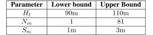
To evaluate PSO performance, we introduce a test case. This case consists in a CRS where heliostats are composed of flat square mirrors as presented in the previous section. We take into account 3 parameters : the height of the tower, the size of mirrors and the number of mirrors by heliostat. The restriction on reflective area is set to 15 000m2. Table 1 presents parameters bounds and Table 2 presents PSO parameters
and results for each test case. Under this circumstances, a complete optimization process is achieved in approximately 1h30min.
Table 1. Parameters symbols, lower bound and upper bound Parameter Lower bound Upper Bound
Ht 90m 110m
Nm 1 81
Sm 1m 3m
4.2 Criteria of comparison
To make a comparison, we introduce some measurements of optimization methods performance. For each run, we calculate the normalized cost reduction defined in Eq.(9) and the distance to the maximum obtained reduction defined in Eq. (10). x∗is the particle with the highest target function for each test case, xbis the reference case a with standard PSO parameters as presented by [14] and ˆx is the iterate with the
highest target function value obtained by any of the tested optimization algorithm. We also want to check how particles converge towards the optimum. To do so, we introduce the mean and the relative standard deviation of the particles target functions.
r(x∗) = f (x ∗) − f (xb) f (xb) (9) d(r(x∗)) = r(ˆx) − r(x∗) =f (ˆx) − f (x ∗) f (xb) (10) 4.3 Optimization performance
As presented in Tab. 2, it appears that results are very close regardless to parameters. In the meanwhile, the use of dynamic inertia leads to the appearance of a better target function optimum. The highest target function, achieved with the Ref. h (GCPSO, c1 = c2 = 1.5, wmin = 0, wmax = 1.2), is evaluated to
25.25GWh. The standard PSO (Ref. a) reaches the value of 25.22GWh and the Ref. b (PSO, c1= c2=
0.5, wmin= 0, wmax= 1.2) represents the more efficient PSO with a target function value of 25.24GWh.
Table 2. Parameters of PSO algorithms, normalized cost reduction and distance to the maximum obtained cost reduction
Reference Type of PSO c1value c2value wminvalue wmaxvalue r(x∗) d(r(x∗))
a PSO 2 2 1 1 0.00% 0.32% b PSO 0.5 0.5 0 1.2 0.31% 0.01% c PSO 1 1 0 1.2 −0.23% 0.55% d PSO 1.5 1.5 0 1.2 0.23% 0.09% e PSO 2 2 0 1.2 0.23% 0.09% f GCPSO 0.5 0.5 0 1.2 0.06% 0.26% g GCPSO 1 1 0 1.2 0.00% 0.32% h GCPSO 1.5 1.5 0 1.2 0.32% 0.00% i GCPSO 2 2 0 1.2 0.06% 0.09% 4.4 Rate of convergence
To investigate swarm’s convergence, we compare the standard PSO a with test cases b and h which obtain the highest target function value for respectively PSO and GCPSO algorithms. Fig. 2 represents swarm’s mean for test cases a, b and h and Fig. 3 represents swarm’s relative standard deviation for these 3 cases. We observe an erratic behavior for each case due to the non-smooth characteristic of the target function on both charts. However, the introduction of a dynamic inertia weight results in less irregular curve as observed for test cases b and h. Although best target functions values obtained with different PSO parameters are very close, as presented at section 4.3, the target function is highly unsmooth, making swarm convegence difficult to achieve.
1.9e+07 2e+07 2.1e+07 2.2e+07 2.3e+07 2.4e+07 2.5e+07 5 10 15 20 25 30 35 40 45 50 Mean (kWh) Number of realizations a b h
Fig. 2. Mean of swarm’s target functions for test cases a, b and h
4.5 PS10 redesign
As a validation case, we present a comparison between a model built using PS10 specifications (624 heliostats of 120m2and a 115m tower) and the result of an optimization run constrained by the PS10 land
2 4 6 8 10 12 14 16 18 20 5 10 15 20 25 30 35 40 45 50 Relati v e standard de viation (%) Number of iterations a b h
Fig. 3. Relative standard deviation of swarm’s target functions for test cases a, b and h
surface area. The following conditions are set :
• Heliostats are made of flat mirrors with square facets;
• Heliostat field follows a radial staggered layout according to the MUEEN method ;
Design parameters for optimization are the number of mirrors composing each heliostat and the width of each mirror. Doing so, the surface of mirrors can be significantly different. We compute this example with our tool. At the end of the process, the overall performance of the obtained CRS is increased by 14% compared to PS10 based CRS (annual thermal energy collected increasing from 113.8GWhth to
130GWhth). This optimization routine is run during a reasonable computational time 4h.
5. CONCLUSIONS AND FUTURE WORK
This paper introduced a new approach to design solar central receiver systems by coupling particle swarm optimizer and Monte Carlo method. The design tool developed is based on the maximization of the annual energy at the entrance of a solar receiver. This target function is highly non-smooth, making difficult to obtain a swarm convergence. A validation case is run using PS10 specifications to illustrate efficiency of the method presented. The redesign of this CRS leads to a significant improvement up to 14% of the annual thermal energy collected. In forthcoming work, the PSO algorithm will be hybridized with a Hookes-Jeeves algorithm in order to better accommodate the non-smooth characteristic. Moreover, the direct model will integrate the estimation of the electricity produced and the CRS plant investment cost so as to optimize the power production cost rather than the annual thermal energy collected. The Monte Carlo algorithm will be extended to estimate the production of a thermal cycle. We will also investigate the use of Kriging and metamodels in order to save computational time and increase the number of iterations and the size of swarms.
References
1. G. J. Kolb, S. A. Jones, M. W. Donnelly, D. Gorman, R. Thomas, R. Davenport, and R. Lumia, “Heliostat cost reduction study,” tech. rep., 2007.
2. M. Sánchez and M. Romero, “Methodology for generation of heliostat field layout in central receiver systems based on yearly normalized energy surfaces,” Solar Energy, vol. 80, no. 7, pp. 861 – 874, 2006.
3. X. Wei, Z. Lu, Z. Lin, H. Zhang, and Z. Ni, “Optimization procedure for design of heliostat field layout of a 1mwe solar tower thermal power plant,” in SPIE, vol. 6841, p. 684119, 2007.
4. R. Pitz-Paal, N. B. Botero, and A. Steinfeld, “Heliostat field layout optimization for high-temperature solar thermochemical processing,” Solar Energy, vol. 85, no. 2, pp. 334–343, 2011.
5. C. J. Noone, M. Torrilhon, and A. Mitsos, “Heliostat field optimization: A new computationally effi-cient model and biomimetic layout,” Solar Energy, vol. 86, no. 2, pp. 792 – 803, 2012.
6. J. De La Torre, G. Baud, J. Bézian, S. Blanco, C. Caliot, J. Cornet, C. Coustet, J. Dauchet, M. El Hafi, V. Eymet, R. Fournier, J. Gautrais, O. Gourmel, D. Joseph, N. Meilhac, a. Pajot, M. Paulin, P. Perez, B. Piaud, M. Roger, J. Rolland, F. Veynandt, and S. Weitz, “Monte Carlo advances and concentrated solar applications,” Solar Energy, May In Press, 2013.
7. E. J. Hoogenboom, “Zero-variance monte carlo schemes revisited,” Nuclear science and engineering, vol. 160, no. 1, pp. 1–22, 2008.
8. A. De Lataillade, S. Blanco, Y. Clergent, J. Dufresne, M. El Hafi, and R. Fournier, “Monte carlo method and sensitivity estimations,” Journal of Quantitative Spectroscopy and Radiative Transfer, vol. 75, no. 5, pp. 529–538, 2002.
9. M. Pharr and G. Humphreys, Physically Based Rendering, second edition : from theory to implemen-tation. Morgan Kaufmann Publishers, 2010.
10. R. Osuna, V. Fernandez, M. Romero, and M. J. Marcos, “Ps10 : A 10 mw solar thermal power plant for southern spain,” in Proceedings of 10th SolarPACES Conference, (Sydney, Australia), July 2000. 11. F. M. F. Siala and M. E. Elayeb, “Mathematical formulation of a graphical method for a no-blocking
heliostat field layout,” Renewable energy, vol. 23, no. 1, pp. 77–92, 2001.
12. M. Roger, M. El Hafi, R. Fournier, S. Blanco, A. De Lataillade, V. Eymet, P. Perez, and É. d. M. d. Carmaux, “Applications of sensitivity estimations by monte carlo methods,” in The 4th International Symposium on Radiative Transfer, 2004.
13. M. Wetter and J. Wright, “A comparison of deterministic and probabilistic optimization algorithms for nonsmooth simulation-based optimization,” Building and Environment, vol. 39, no. 8, pp. 989–999, 2004.
14. J. Kennedy and R. Eberhart, “Particle swarm optimization,” in Neural Networks, 1995. Proceedings., IEEE International Conference on, vol. 4, pp. 1942–1948, IEEE, 1995.
15. F. Van Den Bergh and A. P. Engelbrecht, “A new locally convergent particle swarm optimiser,” in Systems, Man and Cybernetics, 2002 IEEE International Conference on, vol. 3, pp. 6–pp, IEEE, 2002.