Development and calibration of indicators of the quality of agricultural soils of the South of China

(1)

HAL Id: tel-00810547

https://tel.archives-ouvertes.fr/tel-00810547

Submitted on 10 Apr 2013

HAL is a multi-disciplinary open access archive for the deposit and dissemination of sci-entific research documents, whether they are pub-lished or not. The documents may come from

L’archive ouverte pluridisciplinaire HAL, est destinée au dépôt et à la diffusion de documents scientifiques de niveau recherche, publiés ou non, émanant des établissements d’enseignement et de

Development and calibration of indicators of the quality

of agricultural soils of the South of China

Li Liu

To cite this version:

Li Liu. Development and calibration of indicators of the quality of agricultural soils of the South of China. Agricultural sciences. Université Pierre et Marie Curie - Paris VI, 2007. English. �NNT : 2007PA066629�. �tel-00810547�

(2)

UNIVERSITE PIERRE ET MARIE CURIE

THESE DE DOCTORAT DE LUNIVERSITE PARIS 6

Spécialité Sciences de la Vie

Présentée par

Li LIU

Pour obtenir le grade de

DOCTEUR de lUNIVERSITE PARIS 6

Mise au point et calibration d'indicateurs de la qualité de

sols agricoles du Sud de la Chine

Soutenue le 18 juillet 2007 devant le jury composé de :

M. Eric BLANCHART Rapporteur

M. Thibaud DECAENS Rapporteur

Mme. Elena VELASQUEZ Examinateur

M. Luc ABBADIE Examinateur

M. BaoGui ZHANG Directeur de thèse

(3)

Catalogue

Chapter I: Assessment of soil quality in different types of land-use General Indicator of Soil Quality in South China

Résumé...2

Abstract.4

I.1 General Introduction..6

I.1.1 The concept of soil quality (SQ) ....6

I.1.2 Soil quality indicators7

I.1.3 Brief introduction of soil degradation in China ..10

I.2 Sampling protocols and treatments 17

I.2.1 Sites description and sampling 17

I.2.2 Statistic analysis...19

I.3 Physical properties22

I.3.1 Introduction..22

I.3.2 Materials and methods..24

I.3.3 Results and discussion..24

I.3.3.1 Soil texture.24

I.3.3.2 Soil bulk density... 25

I.3.3.3 Soil strength...26

I.3.3.4 Soil water content..27

I.3.4 Multivariate analyses (PCA) of physical parameters...27

I.3.5 Calculation of the Physical sub-indicator.30

I.3.5.1 Selection of the most discriminating variables and homothetic transformation of original data between 0.1-1.0...30

I.3.5.2 Design of the physical sub indicator...31

I.4 Chemical properties..32

I.4.1 Introduction..32

I.4.2 Materials and methods..33

I.4.3 Results and discussion..33

I.4.3.1 Soil pH...33

I.4.3.2 Exchangeable K+...34

I.4.3.3 Exchangeable Ca2+35

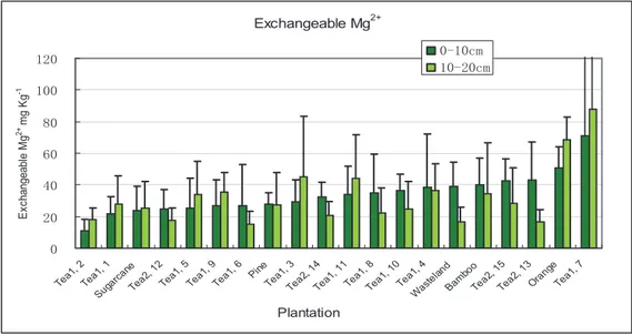
I.4.3.4 Exchangeable Mg2+...35

I.4.4 Multivariate analyses (PCA) for chemical parameters..36

I.4.5 Calculation of the chemical sub-indicator...39

I.5 Soil organic matter (SOM) properties41

I.5.1 Introduction...41

I.5.2 Materials and methods...42

I.5.3 Results and discussion...43

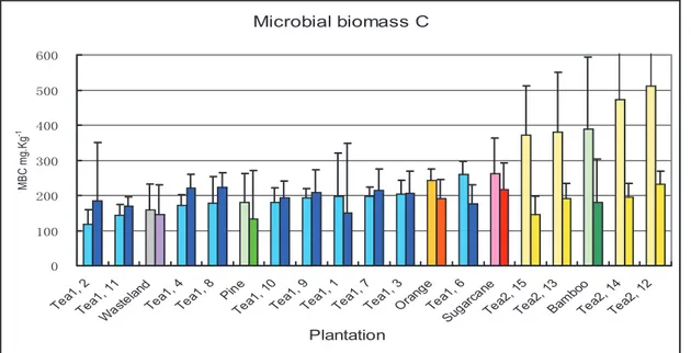
I.5.3.1 Soil microbial biomass carbon....43

(4)

I.5.3.5 Soil nitrate...46

I.5.4 Multivariate analyses (PCA) for soil organic matter parameters.47

I.5.5 Calculation of the soil organic matter sub-indicator...50

I.6 Soil Macrofauna....52

I.6.1 Introduction...52

I.6.2 Materials and methods.....55

I.6.3 Results and discussion...55

I.6.4 Multivariate analyses (PCA) for soil macrofauna...56

I.6.5 Calculation of the soil macrofauna sub-indicator...60

I.7 Soil morphology....62

I.7.1 Introduction....62

I.7.2 Method of soil morphology assessment...63

I.7.3 Results and discussion....65

I.7.4 Multivariate analyses (PCA) for soil morphology......66

I.7.5 Calculation of the soil morphology sub-indicator......68

I.8 General indicator of soil quality (GSQI) ....70

I.8.1 Multivariate analyses (PCA) for sub-indicator.....70

I.8.2 Calculation of the general indicator of soil quality...73

I.9 Ability of IGQS to assess changes occurred after soil restoration76

I.9.1 The (FBO) fertilisation Bio-Organic technology....76

I.9.2 Soil sub-indicators calculation.....77

I.10 Discussion and conclusion In English....83

Chapter : Assessment of soil structure in different types of land-use stable aggregates and soil morphology Résumé....... ... ...89

Abstract.......91

.1 General introduction.........93

.1.1 Basic concepts of soil structure, a key factor in soil function.....93

.1.2 Soil structure formation and factors affecting these processes......94

.1.3 Main methods for the study of soil structure.......98

. 2 Site characterisation......100

.2.1 General characterisation.....100

.2.2 Basic biological, physical and chemical properties......101

. 2.2.1 Soil microbial biomass carbon.......101

C. 2.2.2 Soil respiration for 7 days......102

C. 2.2.3 Ratio of soil respiration and microbial biomass carbon....102

. 2.2.4 Total carbon.......103

(5)

.2.3 Multivariate analyses (PCA) for basic biological, physical and chemical

properties..........105

.3 Aggregates stability analysed by method of wet-sieving.......107

エ.3.1 Basic concept of aggregation..........107

エ.3.2 Methods to assess soil aggregate size distribution and stability..113

エ.3.3 Wet-sieving method utilised in our study.........113

C.3.4 Results and discussion.......118

C.3.4.1 Aggregation in the 0-10 cm soil layer.......118

エ.3.4.2 Aggregation in the 10-20 cm soil layer.........121

エ.3.5 Near infrared reflectance spectroscopy (NIRS) ........125

.4 Soil morphology properties.......128

エ.4.1 Basic concept of soil morphology and micromorphology......128

C.4.2 Results and discussion..........133

エ.4.2.1 Variation of soil morphological composition...133

エ.4.2.2Multivariate analyses (PCA) for soil morphology in the 6 studied sites..134

.5 Soil aggregate stability distribution analysis by wet-sieving after morphological separation........137

エ.5.1 Method and material.........137

エ.5.2 Results and discussion..........138

.6 Discussion and conclusion En français....140

In English......145

Reference.......150

(6)

Figures List

Figure I.1: soil degradation from City to City +200km in China. .......11

Figure I.2: Wind Erosion in China. .........12

Figure I.3: Water Erosion in North China. ........12

Figure I.4: Water Erosion in South China.13

Figure I.5: Chemical Deterioration in China.......14

Figure I.6: Location of the study sites. .........17

Figure I.7: Variations of soil texture e among the20 sites. The first columns of each site are values for soil samples taken from 0-10 cm and second columns are values for soil samples taken from 10-20 cm. ....25

Figure I.8: Variations of soil bulk density among the 20 sites (0-5 cm depth). ..25

Figure I.9: Variations of soil strength among the 20 sites. The first columns of each site are values for measurements done at 0-10 cm, second columns at 10-20 cm and third column, at 20-30 cm. .......26

Figure I.10: Variations of water content among the 20 sites...27

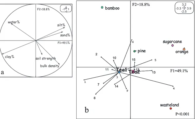
Figure I.11: Ordination of sites by PCA analysis of bulk density, water content, soil strength, sand, silt and clay content..........29

(a) Correlation circle of variables with factors 1 and 2 of PCA analysis with the 6 physical parameters (b) Projection of sites in the plane defined by factors 1 and 2. Circles indicate barycentres related by arrows to sites with a common type of land use. p is probability for groups not to be different (permutation test with 10000 repetitions). P: probability for separation among groups was significant. Factors 1 and 2 explain together 67.9% of the inertia. Figure I.12: Variations of soil pH among the 20 sites. The first columns of each site are values for soil samples taken from 0-10 cm and second columns are value for soil samples taken from 10-20 cm. .......33

Figure I.13: Variations of soil exchangeable K+ among the 20 sites. The first column of each site are values for soil samples taken from 0-10 cm and second columns are value for soil samples taken from10-20 cm. ......34

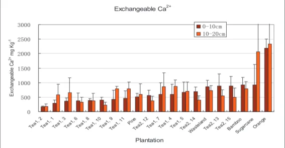
Figure I.14: Variations of soil exchangeable Ca2+ among the 20 sites. The first column of each site are values for soil samples taken from 0-10 cm and second columns are value for soil samples taken from 10-20 cm. ..35

Figure I.15: Variations of soil exchangeable Mg2+ values in the 20 sites. The first column of each site are values for soil samples taken from 0-10 cm and second columns are value for soil samples taken from 10-20 cm. ..36

Figure I.16: Ordination of sites by PCA analysis of soil pH, exchangeable K+, Ca2+and

(7)

the 4 chemical parameters.

(b) Projection of sites in the plane defined by factors 1 and 2. Circles indicate barycentres related by arrows to sites with a common type of land use. p is probability for groups not to be different (permutation test with 10000 repetitions).

P: probability for separation among groups was almost significant. Factors 1 and 2 explain together 87.9% of the inertia.

Figure I.17: Variations of microbial Biomass Carbon among the 20 sampling sites. The first columns of each site are values for soil samples taken from0-10 cm

and second columns are value for soil samples taken from10-20 cm. 43

Figure I.18: Variations of total carbon content among the 20 sites. The first columns of each site are values for soil samples taken from 0-10 cm, second columns are value for soil samples taken from 10-20 cm and third column are values

for soil samples taken from 20-30 cm. 44

Figure I.19: Variations of nitrogen content among the 20 sites. The first columns of each site are values for soil samples taken from 0-10 cm, second columns are value for soil samples taken from 10-20 cm and third column are values for

soil samples taken from 20-30 cm. ..45

Figure I.20: Variations of soil ammonium concentration among the 20 sites. The first columns of each site are values for soil samples taken from 0-10 cm depth,

second columns represent 10-20 cm depth. 46

Figure I.21: Variations of soil nitrate concentration among the 20 sites. The first columns of each site are values for soil samples taken from 0-10 cm depth,

second columns are values for soil samples taken from 10-20 cm. 47

Figure I.22: Ordination of sites by PCA analysis of soil microbial biomass carbon, total carbon content, total nitrogen content, ratio of microbial biomass carbon

(MBC) and total carbon content, Ammonium, Nitrate. ..49

(a) Correlation circle of variables with factors 1 and 2 of PCA analysis with the 6 SOM parameters.

P: probability for separation among groups was significant. Factors 1 and 2 explain together 69.7% of the inertia.

Figure I.23: Variations of soil macrofauna density and composition among the 20

sites (mean values of 5 points). 55

Figure I.24: Ordination of sites by PCA analysis of soil 16 orders of soil

macrofauna....59

(a) Correlation circle of variables with factors 1 and 2 of PCA analysis with the 16 orders of soil macrofauna.

(8)

repetitions).

Figure I.25: Variations of soil morphological composition among the 20 sites...66

Figure I.26: Ordination of sites by PCA analysis of soil morphological items68

(a) Correlation circle of variables with factors 1 and 2 of PCA analysis with the 11 soil morphological items.

Factors 1 and 2 explain together 38.9% of the inertia.

Figure I.27: Ordination of sites by PCA analysis of chemical, physical, soil organic

matter, soil macrofauna and soil morphology sub-indicators. .72

(a) Correlation circle of variables with factors 1 and 2 of PCA analysis with the 5 sub-indicators.

(b) Projection of sites in the plane defined by factors 1 and 2. Small circles indicate barycenters related by arrows to sites with a common type of land use. p is probability for groups not to be different (permutation test with 10000 repetitions).

P: probability for separation among groups was significant. Factors 1 and 2 explain together70.2% of the inertia.

Figure I.28: Effect of application of the FBO technology on soil macroinvertebrate communities (bars are average of densities m² of invertebrates extracted from three 25x25x30cm monoliths, in three replicated plots per treatment).

Numbers on top of columns indicate richness in different order of macrofauna

(data Nuria Ruiz)..78

Figure I.29: PCA analysis of macrofauna data collected in October 2005. T1 : FBO 100%; T2 and T3: FBO with 50% mineral fertilization; T4: Conventional

management. IN: inside FBO trenches; OUT: outside trenches..79

Figure I.30: Aggregation of soil in conventional treatment and FBO trenches (data

Elena Velasquez)...80

Figure I.31: Projection of treatments in factorial plane defined by the main two factors. C0: values before onset of experiment; C6 and C12: plots maintained with conventional management; T6 and T12: FBO trenches at 6 and 12 months respectively; O6 and O12: outside FBO trenches in plots with FBO management, 6 and 12 months respectively after the onset of the experiment. P:

permutation test on PCA coordinates82

Figure .1: Factors affecting soil aggregation (Bronick and Lal, 2005). 95

Figure .2: Regulations of decomposition in the drilosphere, Source: Lavelle, 1997..97 Figure .3: Variations of soil microbial biomass C among the six sites sampled.101

(9)

Figure .5: Variations of ratio of Soil respiration and Soil microbial biomass C

among the six sites sampled. ..102

Figure .6: Variations of total soil carbon content among the six sites

sampled...103

Figure .7: Variations of soil bulk density among the six sites sampled. 104

Figure .8: Variations of soil texture among the six sites sampled. .104

Figure .9: Variations of soil pH among the six sites sampled. 105

Figure .10: Projection of sites in factorial space defined by PCA analysis of basic physical, chemical and soil organic matter properties, including soil texture, bulk density, soil pH, soil respiration (7 days), total C and microbial biomass

carbon. .106

(a) Correlation circle of soil variables with factors 1 and 2 of PCA analysis (b) Projection of sites in the plane defined by factors 1 and 2. Circles

indicate barycentres related by arrows to sites with a common type of land use. p is probability for groups not to be different (permutation test with 10000 repetitions).

Figure .11: The opposing chronology of the formation of the hierarchical aggregate orders implicitly described by Tisdall and Oades (1982) vs. postulated by

Oades (1984). ..108

Figure .12: The conceptual model of the life cycle developed by Six et al., (1998).

Figure is adopted from Six et al. (2000a). ...109

Figure .13: A general model of processes and agents involved in the formation of

aggregates. ...111

Figure .14: Experimental procedure used to assess aggregate stability.. 115

Figure .15: Variation of aggregate distribution for samples taken from 0-10 cm

among the 6 sites (means of two repetitions). 118

Figure .16: Ordination of sites by PCA analysis of different aggregate

diameters.119

(a) Correlation circle of variables with factors 1 and 2 of PCA analysis with the 5 aggregate diameters.

Figure .17: Ordination of site by PCA analysis of basic physical, chemical, soil

organic matter properties and GMD. ..120

(a) Correlation circle of variables with factors 1 and 2 of PCA analysis with the 9 parameters.

(b) Projection of sites in the plane defined by factors 1 and 2. Circles indicate barycentres related by arrows to sites with a common type of land

(10)

Figure .18: Variation of aggregate distribution for samples taken from 10-20 cm

among the 6 sites (means of two repetitions)...121

Figure .19: Ordination of sites by PCA analysis of different aggregate

diameters..122

(a) Correlation circle of variables with factors 1 and 2 of PCA analysis with the 5 aggregate diameters.

Figure .20: Ordination of site by PCA analysis of basic physical, chemical, soil

organic matter properties and GMD. .. 123

(a) Correlation circle of variables with factors 1 and 2 of PCA analysis with the 9 parameters.

(b) Projection of sites in the plane defined by factors 1 and 2. Circles indicate barycentres related by arrows to sites with a common type of land use. p is probability for groups not to be different (permutation test with 10000 repetitions), MBC: Microbial Biomass C.

Figure .21: Variation of geometrical diameter among the 6 studied sites...124

Figure .22: Result of soil NIRS analysis. Projection of aggregates of different diameters in factorial space defined by PCA analysis of different wave length (samples taken from 0-10cm). 0.5-1 was aggregate which diameter between 0.5 and 1 mm, 0.25-0.5 was aggregate which diameter between 0.25 and 0.5 mm, 0.05-0.25 was aggregate which diameter between 0.05 and

0.25 mm. .126

(a) Correlation circle of variables with factors 1 and 2 of PCA analysis, with wave lengthes from 1100 nm to 2440 nm, granularity was 20 nm.

(b) Projection of aggregates with different diameters form the 6 sites in the plane defined by factors 1 and 2.

Figure .23: Soil structure, including soil architecture, over several orders of magnitude (<µm to >cm) from soil profile in the field to microscopic level along with some related soil processes and conditions (Carter, 2004)131

Figure .24: Photographs of some components of the soil matrix in topsoil profiles

(Topoliantz et al, 2000). ..132

(11)

components.135

(a) Correlation circle of variables with factors 1 and 2 of PCA analysis with the 13 soil morphology components.

P: probability for separation among groups was significant. The six tea blocks could be separated significantly. Factors 1 and 2 explain together 37.9% of the inertia.

Figure .27: Ordination of sites by PCA analysis of 13 soil morphology components

and all the soil basic properties had analysed. 136

(a) Correlation circle of variables with factors 1 and 2 of PCA analysis with the 13 soil morphology components and all the soil basic properties had analysed.

Figure .28: Experimental procedure used to assess water-stable aggregates

distribution after soil morphology analysis. 137

Figure .29: GMD of different morphological aggregates in the 6 sites. .138

(12)

Tables List

Table I.1: Sampling sites description18

Table I.2: Physical soil quality indicators recommended or used by soil researchers

(Schoenholtz et al, 2000.) ..23

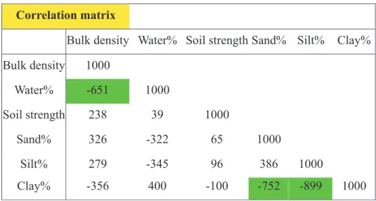
Table I. 3: Correlation matrix of the 6 physical parameters measured in the 20 sites

(rx1000). 28

Table I.4: Inertia of Principal components of soil physical parameters analysed in the

20 sites. ..28

Table I.5: Absolute contributions of the first two principal components of all physical variables analysed in the 20 sites (all contributions are in 1/10000)..28

Table I.6: 4 chemical parameters selected. ..32

Table I.7: Correlation matrix of the 4 chemical parameters measured in the 20 sites

(rx1000). 37

Table I.8: Inertia of Principal component of soil chemical parameters analysed in the

20 sites37

Table I.9: Absolute contributions of the first two principal components of all chemical variables analysed in the 20 sites (all contributions are in 1/10000)..37

Table I.10: Parameters selected as indicators of the organic status of soils.42

Table I.11: Correlation matrix of the 6 SOM parameters measured in the 20 sites

(rx1000). 48

Table I.12: Inertia of Principal component of soil SOM parameters analysed in the 20

sites. ...48

Table I.13: Absolute contributions of the first two principal components of all SOM variables analysed in the 20 sites (all contributions are in 1/10000)..49

Table I.14: Soil macrofaunal orders found in the 20 sites sampled in the Yingde

region. 54

Table I.15: Correlation matrix of the 16 orders of soil macrofauna measured in the 20

sites (rx1000). 57

Table I.16: Inertia of Principal component soil macrofauna measured in the 20 sites.

58

Table I.17: Absolute contributions of the first two principal components of 16 orders of soil macrofauna analysed in the 20 sites (all contributions are in

1/10000). 58

Table I.18: The 11 items used to assess soil morphology (after Velasquez et al., 2006).

63

Table I.19: Inertia of Principal component of 11 soil morphological items studied in

the 20 sites. 67

Table I.20: Absolute contributions of 11 soil morphological items studied in the 20 sites to the first two principal components (all contributions are in

(13)

Table I.22: Correlation matrix of the 5 sub-indicators in the 20 sites (rx1000)...71

Table I.23: Inertia of Principal component of the 5 sub-indicators in the 20 sites...71

Table I.24: Absolute contributions of the first two principal components of the 5 sub-indicators at the 20 sites (all contributions are in 1/10000). ...72

Table I.25: Coefficients of the five sub-indicators73

Table I.26: General indicator of soil quality (GSQI) of the 20 sites. ...74

Table I.27: values of the five sub indicators and General Indicator of Soil Quality, at the onset of the FBO application, after 6 months, inside and outside the trenches, and after 12 months (data and calculations provides by Elena Velasquez and Nuria Ruiz). Underscored values are higher than values in

conventional treatment taken at the same time...81

Table .1: Sampling sites description and values of the General Indicator of Soil

Quality (GISQ) in the 2004 sampling. .100

Table .2: Soil structure in temperate soils: agents in structure formation and

stabilization, processes involved, and scale of structure (Carter and Stewart,

1996). 110

Table .3: Summary of indices proposed for quantitatively assessing soil aggregate stability. n is the total number of aggregate size classes (Marquez et al.,

2004). ...117

Table .4: Average geometrical diameter of the 6 studied sites and their fertilizer

application. ..124

Table .5: Emerging levels of soil structural and functional complexity in agricultural

systems130

Table .6: 13 visual components of soil morphology133

Annexe Table 1: Physical properties: 6 variables (mean values of 5 points). Absolute highest and minimum values are marked with green and yellow colour

respectively. .172

Annexe Table 2: Reduced physical parameter values and sub-indicator. ..174

Annexe Table 3: Chemical properties: 4 variables (mean values of 5 points). Absolute highest and minimum values for each depth are marked with green and

yellow colour. ..175

Annexe Table 4: Reduced chemical parameter values and sub-indicator. .176

Annexe Table 5: SOM properties: 6 variables (mean values of 5 points). Absolute highest and minimum values are marked with green and yellow colour

..177

Annexe Table 6: Reduced SOM parameters and sub-indicator. 179

Annexe Table 7: Soil macrofauna density (ind m-2) at the 20 sites (mean values of 5

points). Absolute highest values were marked with green colour180

Annexe Table 8: Reduced soil macrofauna density values and sub-indicator181

Annexe Table 9: 11 Separation of soil among morphological items at the 20 sampled sites (relative units obtained by grid counting). Absolute highest values

(14)

Annexe Table 12: Weights of different aggregate diameters fractions and values of GMD (Soil samples taken from depth of 0-10 cm, average values of the two

sub-samples). ..185

Annexe Table 13: Fractions weights of different aggregate diameters and values of GMD (Soil samples taken from depth of 10-20 cm, average values of the two

sub-samples). 186

Annexe Table 14: 13 variables of soil morphology of the 6 sites (5 points in each

site)..187

Annexe Table 15: Aggregates distribution (%) of large, medium size and small biogenic and physical aggregates, each site had 5 points (blank means there

was no this kind of aggregate from morphology analysis)..188

Annexe Table 16: GMD (mm) of large, medium size and small biogenic and physical aggregates, each site had 5 points (blank means there was no this kind of

(15)

I

"

Assessment of soil quality ! General Indicator of Soil

Quality in plantations in South of China

(16)

Résume

Un système d"indicateurs de la qualité des sols a été mis au point pour comparer l"effet des types de gestion des sols dans une région du Sud de la Chine. Ce système synthétise en 5 sous indicateurs et un indicateur général la nature complexe du système sol qui exige la prise en compte simultanée des aspects physique, chimique et biologique. Les méthodes statistiques multivariées sont utilisées ici pour traiter des tableaux de données comportant des dizaines de variables différentes.

On a évalué la qualité du sol dans la région de YingDe, (Province de Canton dans le sud de Chine), sur 20 parcelles avec différents type d"utilisation du sol: plantations de thé à différents degrés d"intensification (labour et fertilisation), plantation d"orangers, de canne à sucre, de bambou et de pin.

Un ensemble de paramètres mesure l"état physique, chimique, la qualité et quantité de matière organique, l"aggrégation et la morphologie du sol superficiel (0 à 5 cm), ainsi que la diversité et la composition de la communauté de macroinvertébrés du sol. Ces 5 sous-indicateurs (physique, chimique, matière organique, morphologique, biodiversité) sont ensuite regroupés pour former un indicateur général de la qualité du sol (IGQS).

Le diagnostic ainsi effectué montre des différences significatives entre la nature des plantations, entre les méthodes de gestion et l"ancienneté des diverses plantations de thé. Les plantations de thé recevant les plus grands apports de résidus organique et de fumier ont des valeurs d" IGQS plus élevées que celles qui reçoivent de l"urée comme apport azoté, La plantation d"orangers fertilisée avec du fumier, de la chaux et et du N, P, K comme fertilisants a la valeur d"IGQS la plus élevée des 20 sites. Comparé aux pratiques recourant à la fertilisation chimiques et à l"utilisation de pesticides chimiques, l"apport de fumiers ou résidus organiques, combiné à la lutte naturelle contre des insects nuisibles améliore beaucoup la qualité du sol ainsi que le recyclage du carbone. Le sous-indicateur de morphologie du sol semble être affecté par le type d"engrais.

(17)

La matière organique est le facteur le plus important dans la détermination de la qualité du sol. Des apports importants favorisent la diversité, l"abondance et l"activité des invertébrés ; ceux ci produisent plus d"agrégats biogéniques qui peuvent exercer leurs effets à long terme sur les divers services écosystémiques du sol. Le sous indicateur chimique est apparu très sensible aux applications de fumier, d"engrais chimique ou de chaux. A l"inverse, l"indicateur physique est moins fluctuant, la teneur en argile étant la principale variable qui discrimine les sites sur des critères physiques.

Mots clés : Indicateur général de la qualité du sol ; Analyse de Composantes principales ; macrofaune du sol ; morphologie du sol

(18)

Abstract

Soil quality research differs from some soil management research in that it emphasizes the multifaceted nature of soils and requires that physical, chemical, and biological aspects of the soil be considered simultaneously. Unsupervised methods of multivariate statistics are powerful tools for this integrated assessment and can help soil researchers to extract much more information from their data. In our study, soil quality indicator is constructed by divers measured properties by this technique. Soil quality was assessed on a set of 20 plots submitted to different types of land use, tea plantations with diverse degrees of intensification and fertilizer, orange tree plantation, sugarcane, bamboo forest, pine forest and wasteland in the region of Yingde (Guangdong Province, South China). Our study aimed to design a synthetic indicator that allowed quantifying the physical state, chemical fertility, quality and stocks of organic matter, aggregation and morphology in the surface soil (0 - 5 cm) and diversity and composition of soil macroinvertebrate communities. These 5 sub-indicators (physical, chemical, organic matter, morphological and biodiversity) then are combined into a general index. Significant differences were observed among different plantations and tea plantations with different history and managements by general indicator of soil quality (GISQ). Tea plantations that were replanted and with less residue had lower GISQ than plots that had not been replanted, more residue and manure was applied. Tea plantations with urea had lower GISQ than plots applied manure. Orange plantation with fertilizers of manure, lime and N, P, K had the maximum GISQ. Compared with mineral fertilizers or pesticides, use manures or organic residues could improve soil quality, control pests naturally, improve soil C circulation. Soil morphology sub-indicator seems to be affected greatly by the type of fertilizers applied.

Soil organic matter status is observed to be the crucial factor that determines soil quality, which favors the presence of invertebrate, improves it"s abundance and biodiversity; this results in more biogenic aggregates that are created by invertebrate. Chemical sub-indicator is very sensitive to manure, fertilizer and lime

(19)

application. On the contrary, physical sub-indicator is less dependent on differences of fertilizer application, it is the clay content that most differs the sites.

Keyword: General indicator of soil quality; Principle component analysis; Soil macrofauna; Soil morphology

(20)

I.1 General Introduction

I.1.1 The concept of soil quality (SQ)

Soil is a critically important component of the earth"s biosphere, which supports the production of food, fiber and participate in the provision of a wide range of ecosystem services (Glanz, 1995; MEA, 2005). Thus, the thin layer of soil covering the surface of the earth supports most land-based life (Doran et al., 1996). However, inventories of soil productive capacity indicate human-induced degradation on nearly 40% of the world"s agricultural land as a result of soil erosion, atmospheric pollution, extensive soil cultivation, over-grazing, land clearing, salinization, and desertification (Oldeman, 1994, MEA, 2005). Indeed, degradation and loss of productive agricultural land is one of our most pressing ecological concerns, rivaled only by other human caused environmental problems like global climate change, depletion of the protective ozone layer, and serious declines in biodiversity (Lal, 1998).

Soil quality is essential in sustaining the global biosphere and developing sustainable agricultural practices. Soils are being degraded worldwide through processes of erosion, anaerobiosis, salinization, compaction and hard-setting, organic matter depletion, and nutrient imbalance. Most of these processes are themselves linked to depletion in the diversity and activity of the many species of invertebrates and microbes that operate the different soil functions (Lavelle et al., 2006). Central to sustainable agroecosystems must be the protection and enhancement of soil quality. Soil quality is a measurement of their ability to produce plant biomass, maintain animal health and production, recycle nutrients, store carbon, partition rainfall, buffer anthropogenic acidity, recycle added animal and human wastes.

The concept of soil resource management (separate from crop or forest management) for sustaining the productivity of plant systems is critical to ensure the reality of sustainable agriculture and environmental protection. Measuring soil

(21)

quality, if properly characterized, should serve as an indicator of the capacity of soils to produce safe and nutritious food, enhance human and animal health, and overcome degradative processes (Papendick and Parr, 1992). Therefore, the overall purpose of this renewed emphasis on soil quality is to develop a more sensitive and dynamic way to document soil conditions, how they respond to management, and their resilience to stresses imposed by land use practices.

The Soil Science Society of America (1997) defined soil quality as, #The capacity of a specific kind of soil to function, within natural or managed ecosystem boundaries, to sustain biological productivity, maintain environmental quality, and promote plant and animal health$. Another organization has suggested that, #sustainable agriculture should involve the successful management of resources to satisfy changing human needs while maintaining or enhancing the quality of the environment and conserving natural resources$ (Technical Advisory Committee to the CGIAR, 1988).

I.1.2 Soil quality indicators

The interaction of soil health along with soil stability and soil resilience contributes to the sustainable use of the soil resource (Lal, 1993). Soil health or quality evaluation should be based upon soil functions and indicators that measure these attributes and their interactions. Soil functions would be defined in terms of physical, chemical, and biological properties and processes and measured against some definable standard to determine whether a soil is being improved or degraded (Karlen et al., 1997) by any practice. In turn these attributes describe the soil capacity to perform ecosystem functions such as incorporating, holding and releasing water or energy.

An adequate approach to defining soil quality indicators must be holistic not reductionistic and indicators should thus describe the major ecological processes in soil (Doran and Safley, 1997; Velasquez, in press). Indicators of soil quality should be responsive to management practices, integrate ecosystem processes, and be

(22)

to document the improvement, maintenance or degradation of soil quality (Larson and Pierce, 1994). National and international programs for monitoring soil quality presently include a few general biological indicators such as biomass and respiration measurements, nitrogen mineralization, microbial diversity and functional groups of soil fauna (Bloem et al., 2003).

An indicator of soil quality is a measurable surrogate of a soil attribute that determines how well a soil functions (Burger and Kelting, 1999). Since soils vary naturally in their capacity to fulfill different functions, quality indicators are expected to be relatively specific to each kind of soil. This concept encompasses two distinct although interconnected components, the inherent and dynamic qualities. Characteristics, such as texture, mineralogy, are innate soil properties determined by the factors of soil formation- climate, topography, vegetation and time. Collectively, these properties determine the inherent quality of a soil. They help compare one soil to another and evaluate soil for specific uses (Jenny, 1941; Sanchez et al., 1982). Because these factors are complex and the effects of land-use history may be long lasting, soil quality can be difficult to characterize (Karlen et al., 2001). Soil drainage, tillage, and addition of lime and fertilizer have positive effects on soil productivity, whereas soil erosion, loss of organic matter and physical structure, and other degrading processes have negative impacts. Both positive and negative processes occur simultaneously, making it difficult to associate changing yields with certain cultural practices. More recently, attention has been paid to the dynamics of soil quality defined as the changing nature of soil properties resulting from human use and management (Eijsackers, 1998).

It is often difficult to clearly separate soil functions into chemical, physical, and biological processes because of the dynamic, interactive nature of these processes. This interconnection is especially prominent between chemical and biological indicators of soil quality and there is seldom a one-to-one relationship between function and indicator; more likely, a given function (e.g. sustaining

(23)

soil property or process may be relevant to several soil attributes and/or soil functions simultaneously (Harris et al., 1996; Burger and Kelting, 1999). For example, many soil chemical properties influence microbiological processes and together with soil physico-chemical processes, they determine the capacity of soil to hold and supply water and nutrients. Another good example of the latter is soil organic matter, which plays a role in almost every soil function (e.g. Henderson, 1995; Harris et al., 1996; Nambiar, 1997).

Measurements of soil quality have the potential to reflect the status of soil as an essential resource. To sum up, there are at least five limitations that, if addressed, could bridge the gap between this potential and the current reality described by Jaenicke (1998). (1) Causal relationships between soil quality and ecosystem functions, including biodiversity conservation, biomass production, and conservation of soil and water resources are rarely defined or quantified. True calibration of soil quality requires more than merely comparing values across management systems. (2) Most soil quality indicators have limited power to predict soil responses to disturbance. Although there are many indicators that reflect the current capacity of the soil to function, there are few that can predict the capacity of the soil to support a range of disturbance regimes. (3) Land managers frequently find soil quality monitoring to be inaccessible because the measurement systems are too complex, too expensive, or both. (4) Soil quality measurements are generally presented as &stand-alone" tools. However, in order to be effective, they need to be integrated with other biophysical and socio-economic indicators. (5) Most current soil quality assessments are point-based, yet ecosystems are generally managed at the landscape level.

In soil research"s effort to rate relative performance of a soil in terms of critical functions (whatever the ecological, economical, environmental, or social function(s) we assign to it), we must resort to describing a set of identifiable attributes that such soil must possess in order to perform these functions, and then translate these attributes into first or second-level measurable surrogates (i.e. soil properties or

(24)

number of soil attributes, while any given soil property or process may be relevant to several soil attributes and/or soil functions simultaneously.

I.1.3 Brief introduction of soil degradation in China

This thesis addresses aimed at proposing soil quality indicators for agro ecosystems in Southern China. In the Yingde region, 300 Km north of Guangzhou, land is covered with tea plantations, sometimes 10-30 years old or more, and a mixture of rather diverse cultures, sugarcane, fruit tree plantations (orange), pine forest, separated by bamboo stands or wasteland areas.

Soil degradation is very widespread in China. Since 1978, and the political opening farmland have been cultivated without any interruption and no environmental protective measures. It made the soil seriously degrade and ill irrigation often resulted in salinization (Jiang and Shinaro, 1999). In China, wind erosion mainly happened in north China, concentrated in northest and northwest China (Figure I.1) and the extent of wind erosion (Figure I.2) (Jiang and Shinaro, 1999) were moderate to common in most provinces, the major causes of wind erosion belonged to the agricultural activities, deforestation and overgrazing. From Figure I.1 we can see that from city to city +50km, no matter what type soil degradation, water erosion, wind erosion, chemical deterioration and physical deterioration, the degree and extent of soil degradation had significantly increased. But from city +50km to city to city +50km, it may be the possibility that human activities of agricultural and industrial production mainly concentrated within city +50km. In view of the causes of soil degradation in China, unreasonable agricultural activities and deforestation around city around city area were the major causes.

(25)

Figur I.1: soil degradation from City to City +200km in China (Jiang and Shinaro, 1999)

e .

(26)

Figure I.2: Wind Erosion in China (Jiang and Shinaro, 1999).

china, but the

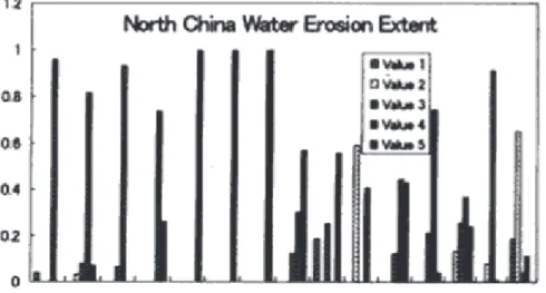
Figure I.3: Water Erosion in North China (Jiang and Shinaro, 1999). Water erosion happened in every province to some extent in

strongest provinces were Hebei province and Tianjin city in north China, the secondary provinces were Jilin and Liaoning provinces in northeast China, the third were provinces located in coastal region in southeast China (Figure I.3 and I.4) (Jiang and Shinaro, 1999).

Heilongjiang Inter Mongolia Xinjiang Liaonin Hebei Gansu Shanxi Shanxi Ningxia Qinghai Tibet Jilin Heilongjiang Inter Mongolia Xinjiang Liaonin Hebei Gansu Shanxi Shanxi Ningxia Qinghai Tibet Jilin

Heilongjiang Inter monkulia Jilin Liaonin Hebei Beijing Tianjin Shanxi Henan Shandong Shanxi Ninxia Gansu Qinghai Xinjiang Heilongjiang Inter monkulia Jilin Liaonin Hebei Beijing Tianjin Shanxi Henan Shandong Shanxi Ninxia Gansu Qinghai Xinjiang

(27)

Figur Water Erosion in South China (Jiang and Shinaro, 1999).

The causes of water erosion were deforestation and agricultural activities, u

Chemical deterioration mainly happened in Hebei, Tianjin, Henan, Xinjiang, Gansu

Jiangsu Anhui ShanghaiZhejinagJiangxi Guangxi Guizhou Sichuan Yuannan Tibet Hunan Hubei Fujian Guangdong Hainan Taiwan Jiangsu Anhui ShanghaiZhejinagJiangxi Guangxi Guizhou Sichuan Yuannan Tibet Hunan Hubei Fujian Guangdong Hainan Taiwan

e I.4:

nreasonable irrigation, overusing groundwater, and it made the soil salinization commonly happen in north China. In northeast China, the major cause of water erosion was overgrazing. The major causes in northwest China is deforestation and in southeast China deforestation and agricultural activities.

, and Inner Mongolia, and in which Hebei province was the most seriously province suffered the chemical deterioration, the secondary provinces ere henna, Shangdong and Xinjiang (Figure I.5). The causes of chemical deterioaration wee unreasonable agricultural activities, overuse groundwater, irrigation and related salinization, etc.

The physical deterioration was limited to Anhui, Henan and Jiangsu provinces; the cause was agricultural activities.

(28)

ation in China. S

f soil under the te

ost of the results are has t

Figure I.5: Chemical Deterior

Inter Mongolia Xinjiang Hebe Beijing Gansu Tianjin Ninxia Shandong Henan Jiangsu Anhui Inter Mongolia Xinjiang Hebe Beijing Gansu Tianjin Ninxia Shandong Henan Jiangsu Anhui

oil in tea gardens in South China had low fertility, this degradation can be seen in the low soil organic matter content, cation exchange capacity, poor and little diverse soil fauna populations and highly acidic pH, and in the high soil compaction, erosion, nutrient leaching. It was similar to the long-term exploitation o

a gardens in Southern India (Panigrahi, 1993; Senapati et al., 1999).

Form the research results, we can get conclusion that in China with economic development, land uses and covers and related environment had greatly been changed. How to rational use land resource and protect the environment as well as keep sustainable development, it is the most important problem that Chinese people has to copy with. In view of analysis and calculated results, m

o copy with. In view of analysis and calculated results, most of the results are consistent with the actual situation. Because of the data belongs to different periods and the difference of the classification criterion, some results are consistent with the actual situation.

Our study aimed to design a synthetic indicator that allowed quantifying the physical state, chemical fertility, quality and stocks of organic matter,

(29)

macroinvertebrate communities. These sub-indicators would then be combined into a gen

action are approached through global measurements of resistance to penetration and shear strength, easy to measure with standard and low cost

ments of cation concentrations and pH allow separating soils with sufficient concentrations in all macronutrients from unfertile, nutri

nic), plants, gravels and stones and ther components to the architecture of the upper cm of soil derived from visual paration of these items. Presence of a large proportion of biogenic aggregates of ifferent sizes rather than physical aggregates or non aggregated soil, invertebrates nd roots linked to high biological activity should indicate high quality soils

lanchart et al., 1999; Ponge, 1999; Topoliantz et al., 2000)

Organic matter is an important attribute of soil quality for the variety of nctions that it has in soils as cation reserve and agent of aggregate stabilization, te for carbon storage and sequestration and as an energetic resource for eterotrophic biological activity. This component of soil quality is assessed through verall contents in C and N, density fractionation that separates short lived light actions from long lived heavy fractions associated to clay and fine silt fractions nd respirometry activities in optimal laboratory incubations that indicate to which xtent organic matter is accessible to soil micro-organisms (Marinissen and

illenaar, 1996; Pulleman et al, 2002; Six et al., 2002).

eral index. The general methodology proposed by Velasquez (2004) was used. Physical quality mainly addresses soil aggregation and the total amount of porosity. General descriptors for this attribute of soil quality are bulk density, total porosity and moisture content that assess void volumes in different ways. Stability of structure and comp

equipments (To and Kay, 2005; Léonard, J and Richard, G. 2004; Larson and Pierce, 1994; Herrick et al., 2001).

Chemical fertility is the ability for soil to provide the basic nutrients necessary to plant growth. Basic measure

ent poor, soils (Larson and Pierce, 1994; Lavelle and Spain, 2006).

Morphology is an assessment of the contribution of soil aggregates of different sizes and origins (physical or bioge

o se d a (B fu si h o fr a e H

(30)

biological activities, the physical and chemical ecosystem engineering operated by icrobial activities (Lee and al., 1997; Pulleman et al., 2005;

rse degrees of intensification and fertilizer, orange tree plantation, sugarcane, bamboo forest, pine forest and wasteland.

a second part, we detailed the physical indicators of soil quality and tried to calibrate the soil morphology indicator, mainly based on a visual assessment of soil aggregation with standard physical methods.

invertebrates themselves, and subsequent associated m Foster, 1991; Pankhurst et al, 1995; Lavelle et

Mathieu et al., 2005).

The implementation of these indicators was done in the region of Yingde, on a set of 20 plots submitted to different types of land use, tea plantations with dive

(31)

I.2 Sampling protocols and treatments

I.2.1 Sites description and sampling

The study sites are located in the Tea Research Institute, Guangdong Academy

of gricu ien d S ea2, 20 km

from Tea e, rov

Location of the study sites.

C te ic ave age

annual sunlight 1700 hours, and an averag inly

concentrated in the arch to August. Soils are clayey, acidic, derived

f

c nt 9% atio

plantation in Tea1 to nge

cm

m c Jun rdens,

1 ar io ard 1 bamboo forest, and a plot

of abandoned land (Table I.1)

fe zer n ag ey are representative of the wide

v tions ed i

sen at s and at the 4 corners

(generally distant 20 ke soil samples.

A ltural Sc ces (Tea1) an hangmingxuan Tea Garden area (T

1), Yingd Guangdong P ince, south of China (Figure I.6).

Figure I.6:

lima is subtrop al, with an rage annual temperature of 20.7@, aver e annual rainfall of 1600 mm, ma period from M

rom Quaternary red clay (Liu, 1993). Surface soil (0-20cm) has a low organic onte (around 1. ), silt/clay r is around 1.0, pH varies from 3.7 in one tea 7.9 in the ora garden, bulk density ranges from 1.0 to 1.5 g

-3

.

Sa pling was arried out in e 2004. 20 sites were selected, 15 tea ga

sug cane plantat n, 1 orange g en, 1 pine forest,

(wasteland) . With different land-use histories,

ements, th

rtili utilizatio and soil man

aria observ n the area.

In each site, 5 points were cho the center of the site to 30 m) to ta

(32)

Table I.1: Sampling sites description.

N° Plantation Location Description

1 Tea1, 1 24°18 24 N,

113°23´19 E 20 years, chemical fertilizer

2 Tea1, 2 24°18 22 N, 3 years, chemical fertilizer and manure*

113°23 01 E

3 Tea1, 3

113°23 01 E 10 years

24°18 21 N,

, chemical fertilizer and manure*

4 Tea1, 4 24°18 21 N,

°23 01 E

10 years, submersed 3 times/10 years, chemical fertilizer and manure*

113

5 Tea1, 5 24°18 21 N,

113°23 01 E

Replanted 2 years ago, chemical fertilizer and manure*

6 Tea1, 6 24°18 24 N,

113°23 19 E 20 years, chemical fertilizer and manure*

7 Tea1, 7 24°18 09 N,

8 Tea1, 8 24°18 09 N,

9 Tea1, 9 24°18 09 N, 10 years, chemical fertilizer and manure*

113°23 08 E

10 Tea1, 10

113°23 01 E 24°18 22 N,

15 years, chemical fertilizer and manure*

11 Tea1, 11 24°18 22 N,

113°23 01 E

15 years, chemical fertilizer and manure*

12 Tea2, 12

113°27 55 E 24°22 13 N,

Nearly 30 years, manure of chicken and cow**

13 Tea2, 13 24°22 13 N,

113°27 55 E

Nearly 30 years, urea and spray fertilizer for leaves***

14 Tea2, 14 24°22 13 N,

113°27 55 E

Nearly 30 years, urea and spray fertilizer fo leaves***

r

15 Tea2, 15 24°22 13 N,

113°27 55 E Nearly 30 years, chicken manure ****

16 Sugarcane 24°17 55 N,

113°23 04 E 3 years, residues

17 Orange 5 years, manure, chemical fertilizer and

113°23 04 E lime****

24°17 55 N,

18 Pine 24°18 21 N,

113°23 01 E

Artificial secondary, less than 10 years, n fertilizer o 19 Bamboo 24°22 13 N, 113°27 55 E 20 years, no fertilizer 20 Wasteland 113°23 01 E 24°18 21 N, No fertilizer

(33)

* Organic manure applied once every 3-4 years, chemical fertilizers 3 times a year and pesticides5-6 times a year

** Chicken and cow manure and P fertilizer applied once a year ***U

Thes

ns of the residual variation. Usually, only the first few PCs

rea and spray fertilizer for leaves were applied 3 times a year **** Manure and fertilizer were applied once year

I.2.2 Statistic analysis

Principal component analysis (PCA, Martens and Naes, 1989) was applied in our data analysis. PCA allows to identify patterns in complex data sets, and express the data in such a way as to highlight their similarities and differences. PCA decomposes a data matrix X of rank h, as a sum of matrices of rank 1. The rank indicates the number of linearly independent vectors of a matrix. The new rank 1 matrices are vector products of the score vectors, t, and loading vectors, p, as shown in Eq:

X = t1p1' + t2p2' +£ £ £+t_hp_h'

e vectors can be calculated by a least squares fit (singular value decomposition<SVD). The new coordinates of the system, named Principal Coordinates, are mutually orthogonal and thus not correlated and successively explain decreasing proportio

account for the greatest amount of total data variance and can be utilized to represent the whole data set in a simpler manner.

The other main advantage of PCA is that once found these patterns in the data, the original set of variables can be reduced into a small number of identified factors without loosing much information.

PCA was used to examine whether disturbed and control plots at different sites differ on the basis of the different sets of variables that were measured in the field. A correlation matrix PCA (correlation circle) was also calculated to reveal relations between variables, and between the variables and the extracted factors.

(34)

processes requires the measurement of many variables and therefore the use of mult

8), assessment of the tillage impacts n soil quality (Wander and Bollero, 1999) or the relation of soil compactibility to hysical and organic properties (Ball et al., 2000). Bentham et al. (1992) used rincipal component analysis and other statistical clustering techniques to choose ariables best representing the progress of soil restoration efforts.

Once the main factors (Principal Components) have been chosen, the data can e projected onto the new reduced space. A score plot depicts the linear projection f objects, allowing the observation of the relative localization and grouping of bjects in factorial spaces.

The correlation of variables is described by the cosine of the angle between the ading vectors. The smaller the angle, the higher the correlation between features. ncorrelated variables are orthogonal to each other. Coordinates along the onsidered PC are a measure of the importance of a feature for the PC model. rojections close to the origin of the coordinate system represent unimportant ariables or items as regards the factors represented. The interactive study of score nd loading vectors, better visualized through the plots, permits the visualization of e influence of each variable on each object (Gabriel, 1971). If a variable is close an object, it likely has a direct influence on it. Conversely, if a variable is distant om an object, it will have high inverse influence on it. The variable and object rojections onto the axes provide their relative contributions for the corresponding

ivariate analytical tools (Sena et al. 2002).

Grouping of analytical data is possible either by means of clustering methods or projecting the high dimensional data onto lower dimensional space. It is obvious that no isolated property can provide an extensive picture of the quality of a specific soil (Torstensson et al., 1998).

The use of PCA and other methods of multivariate analysis has allowed to find the resolution of several problems, for example the determination of management discriminant properties in semiarid soils (Quiroga et al., 1998), identification of sources of soil pollutants (Carlosena et al., 199

o p p v b o o lo U c P v a th to fr p

(35)

The multivariate method PCA was applied to the mean values of variables easured in 5 samples of each site. The data were analyzed using the ADE-4 prog

ysical, soil organic matter, soil acrofauna and soil morphology were calculated based on these results. Finally, a indicator was calculated with all five sub-indicators integrated into

m

ram (Thioulouse et al., 1997). In our study, the five groups of soil parameters (chemical, physical, soil organic matter, soil macrofauna and soil morphology) were analysed by PCA; we calculated how much these parameters distinguish soils from different sites and sub-indicator of chemical, ph

m

general soil quality

(36)

I.3 Physical properties

Physical properties are major indicators of the ability of soils to provide very important ecosystem services; they determine their capacity to infiltrate, store, purify and release water, they also indicate their resistance to erosion and availability of water and air for living organisms.

I.3.1 Introduction

Table I.2 is a list of physical indicators that has been proposed by various researchers (Schoenholtz et al, 2000). Basic soil physical indicators like soil texture and depth may be responsible for different intrinseque soil qualities among soil types.

Soil texture, and especially the amount and quality of clay minerals, is the most fundamental soil physical property controlling water, nutrient, and oxygen exchange, retention, and uptake. The fine soil fraction significantly influences aggregate stability. In coarse-textured soils, soil organic carbon that comprise the only colloid fraction has a greater influence on structure than in fine textured soils; the type of clay may sometimes be more important than the amount in determining aggregation since 2:1 type minerals are better at glueing particles than 1:1 type (Kay, 1998). High clay concentration (and high clay quality, that is predominance of 2:1 type over 1:1) is also associated with increased SOC stabilization (Sollins et al., 1996).

Soil bulk density varies among soils of different textures, structures, and atter content, but within a given soil type, it can be used to monitor the paction and flooding. Changes in soil bulk density affect a host of cesses that ultimately influence water and oxygen supply. easure of soil strength using a cone penetrometer may be the best way root proliferation and growth (Powers et al.,

in a minimum data set of soil quality organic m

degree of soil com other properties and pro However, a m

to index the influence of soil density on 1998). Bulk density is, nonetheless, needed

(37)

(38)

In our study, we selected soil texture, bulk density, soil moisture and soil rength measured with a cone penetrometer to describe soil physical properties.

3.2 Materials and methods

oil samples for texture analysis were take at 0-10 cm and 10-20 cm depth, air- dried and sieved at 2mm. Analysis was done with the pipette method. Soil bulk density was measured on samples collected with 2.5×5 cm annular cylinders; samples were weighted after 24 hours drying in an oven at 105@. Soil moisture was measured

t the same time."Soil strength was measured in site with a cone penetrometer.

I

from .97 to 1.49 in bulk density, 15.1% to 34.1% in water content, 1.76 to 30.58kg

cm-2 t

e tion, 10-20 cm); silt percent varied from 25.9% (Tea1, 1, 10-20 cm) to 58.5% range plantation, 0-10 cm) and clay percent varied from 18.2% (Sugarcane lantation, 10-20 cm) to 62.4% (Tea1, 10-20 cm)(Figure I.7). Overall, soils from the ea 1 area tended to have finer structure that Tea 2 and sites with other types of ropping systems.

st

I. S

a

.3.3 Results and discussion

Physical variables exhibited rather large variations across the sites with values 0

in soil strength, 8.8% to 32.1% in sand percent, 25.9% to 58.5% in silt percen and 18.2% to 62.4% in clay percent (Annexe, Table 1).

I.3.3.1 Soil texture

Sand proportion varied from 8.8% (Tea1, 1, 0-10 cm) to 32.1% (Sugarcan planta

(O p T c

(39)

Figure I.7: Variations of soil texture e among the20 sites.The first columns of each site are values for soil samples taken from 0-10 cm and second columns are values for soil samples taken from 10-20 cm.

Orange plantation had the highest silt percent and Tea plantation Tea1, 8 in tea stitute had the highest clay percent of all the 20 sites.

3.3.2 Soil bulk density

ulk density varied from 0.97g cm-3 in Bamboo to 1.49 g cm-3 in Wasteland (Figure 8).

ute had the highest clay percent of all the 20 sites.

3.3.2 Soil bulk density

ulk density varied from 0.97g cm-3 in Bamboo to 1.49 g cm-3 in Wasteland (Figure 8). in I. I. B B I. I.

Figure I.8: Variations of soil bulk density among the 20 sites (0-5 cm depth). Figure I.8: Variations of soil bulk density among the 20 sites (0-5 cm depth).

Bulk density 3 0 2 2 o Tea1 , 6 Tea1 , 10 Tea2 , 12 Tea2 , 15 Tea1 , 3 Tea1 , 11 Tea1 , 1 Tea1 , 5 Tea2 , 13 Tea2 , 14 Tea1 , 7 Pine ugar cane Tea1 , 8 Tea1 , 2 Oran ge Tea1 , 9 Tea1 , 4 aste land y g 2 0 2 2 2 0 4 2 2 0 6 2 2 0 8 2 2 0 : 2 Bam bo B ul k de ns it 3 0 4 2 3 0 6 2 3 0 8 2 3 0 : 2 c m -3 S W Plantation Soil texture 60% 80% 100% 0% 40% 8 1 7 2 ₁4 ₁1 3 9 ₁0 _oo ₁5 ₁2 6 _ne 5 d 1 3 ₄ S e _ge Plantation 20% T ea 1, T ea 1, T ea 1, T ea 1, T ea 2, T ea 1, T ea 1, T ea 1, T ea 1, B am b T ea 2, T ea 2, T ea 1, _Pi T ea 1, W as te la n T ea 2, T ea 1, ug ar ca n O ra n enc{ uknv ucpf"

(40)

Soil bulk density was around 1.20 g cm-3 for most of the sites. Wasteland had the highest bulk density (1.49 g cm-3) than other sites; this was probably due to its high content in fine sands, limited soil faunal activity and regular flooding (3 times in 10 years). Tea plantation Tea1, 4 in Tea1 had a high bulk density (1.45 g cm-3) probably

ue to its same regular flooding of wasteland.

3.3.3 Soil strength

rgely, from 1.76 (Tea1, 2, 0-10cm) to 30.58 kg cm-2 (Tea1, , 10-20 cm)(Figure I.9).

Tea1, 2 had a very low strength in surface soil; it had been created from few days before our mpling. Site Tea1, 4 had been flooded 3 times in 10 years, which could have made soil h

ength is an important parameter of soil quality for its effect on root proli ation. This parameter however is also dependent on soil moisture and changes d

I.

Soil strength varied la 4 Soil strength 32022 42022 52022 62022 72022 82022 Te Te Te Te _Ba Te Or Te 7 Sug ar e Tea Te Tea Te Te a1, 1 Tea2 , 15 Tea2 , 14 Was tela nd Tea2 , 13 Tea2 , 12 K g 2022 a1, 2 a1, 5 a1, 6 a1, 8_mbo o a1, 3 Pin e ange a1, can 1,11 a1, 4 1,10 a1, 9 Plantation c m -2

Figure I.9: Variations of soil strength among the 20 sites. The first columns of each site are values for measurements done at 0-10 cm, second columns at 10-20 cm and third column, at 20-30 cm.

wasteland 3 years ago, manure was applied at soil surface a sa

arder. Soil str fer