Fusion of High Density Low Precision and Low Density High Precision Data in Coordinate Metrology

(1)

UNIVERSITÉ DE MONTRÉAL

FUSION OF HIGH DENSITY LOW PRECISION AND LOW DENSITY HIGH PRECISION DATA IN COORDINATE METROLOGY

MICHAŁ BARTOSZ RAK

DÉPARTEMENT DE GÉNIE MÉCANIQUE ÉCOLE POLYTECHNIQUE DE MONTRÉAL

ET

FACULTY OF MECHATRONICS WARSAW UNIVERSITY OF TECHNOLOGY

THÈSE EN COTUTELLE PRÉSENTÉE EN VUE DE L’OBTENTION DU DIPLÔME DE PHILOSOPIAE DOCTOR

(GÉNIE MÉCANIQUE) NOVEMBRE 2016

(2)

UNIVERSITÉ DE MONTRÉAL

ÉCOLE POLYTECHNIQUE DE MONTRÉAL

Cette thèse intitulée :

FUSION OF HIGH DENSITY LOW PRECISION AND LOW DENSITY HIGH PRECISION DATA IN COORDINATE METROLOGY

présentée par : RAK Michał Bartosz

en vue de l’obtention du diplôme de : Philosophiae Doctor a été dûment acceptée par le jury d’examen constitué de :

M. ACHICHE Sofiane, Ph. D., président

M. MAYER René, Ph. D., membre et directeur de recherche M. WOŹNIAK Adam, Ph. D., membre et codirecteur de recherche M. FENG Hsi-Yung (Steve), Ph. D., membre

(3)

DEDICATION

I would like to thank my supervisors, Professor Adam Woźniak and Professor René Mayer, for their support and encouragement. Dziękuję Profesorom Wydziału Mechatroniki a w szczególności Pani Dziekan, Profesor Natalii Golnik za otuchę i nadzieję. (translation: I would like to thank professors of the Faculty of Mechatronics, in particular Dean Natalia Golnik for cheer and hope.) Rodzicom i bratu dzięki którym bez obaw wyznaczam sobie kolejne cele, bo wiem, że są ze mną. (translation: I would like to thank my parents and brother who are always with me so I can set new goals without fear.) Ani za ogromną pomoc, motywację i wiarę, gdy mojej brakowało. (translation: Ania thank you for the huge help, motivation

and faith when mine was missing.) Thank you Ania and Xavier for all these splendid days which I spent with you. Najma, je te remercie infiniment pour avoir toujours

réussi à me donner le sourire. (translation: Thank you Najma for always making me smile.)

(4)

RÉSUMÉ

Dans les techniques de mesures tridimensionnelles, les dimensions et la géométrie des éléments sont déterminées sur la base des coordonnées de points. Ces points peuvent être recueillis à partir de méthodes avec ou sans contact. Malheureusement, toutes ces méthodes possèdent aussi bien des avantages que des inconvénients.

Les données issues de mesures sans contact comme la triangulation laser ou les techniques de projection de franges lumineuses se caractérisent par une précision faible, mais une forte densité de points. Les mesures avec contact, quant à elles, produisent des points de faible densité, mais avec une plus grande précision.

Ainsi, il est souhaitable de développer un procédé qui permet la fusion de deux ensembles de données, tout en conservant les avantages et en minimisant les inconvénients.

Cette thèse présente une méthode de fusion, insensible à les caractéristiques des données d'entrée, en particulier dans le cas de mesure sans contact où les propriétés des points recueillis dépendent à la fois de la méthode de mesure et de la stratégie choisie. Ce procédé est applicable pour les surfaces à forme libre.

Dans les méthodes présentées, deux ensembles de données, issues d'une surface, sont recueillis. Un premier ensemble provient de mesure sans contact et fournit des informations complètes sur l'objet mesuré. Le deuxième ensemble résulte de mesures avec contact et représente des points caractéristiques utilisés pour corriger le premier ensemble.

Deux méthodes de détermination des points caractéristiques sont proposées, appelées marqueurs matériels et virtuels. En ce qui concerne les marqueurs matériels, des éléments spéciaux, faits en billes en céramique, sont conçus, fabriqués et montés magnétiquement sur la surface où il est permis. Les centres de ces billes, déterminés à l'aide des données de mesures avec et sans contact, sont des paires de points caractéristiques correspondants, utilisés pour la fusion. Quant aux marqueurs virtuels, les points correspondants sont déterminés à partir de mesure sans contact, sur la base de points recueillis directement sur la surface mesurée, en utilisant la méthode de contact. Ces deux méthodes sont testées sur des pièces industrielles réelles. Pour les marqueurs matériels d'un plan, une aube de turbine et un couvercle de moteur ont été utilisés. En plus, pour les marqueurs virtuels un réservoir de carburant d'un avion a été utilisé. Les résultats de marqueurs

(5)

virtuels sont similaires aux résultats de la simulation par ordinateur. De meilleurs résultats ont été obtenus lorsque la distance entre les points de caractéristique était plus bas. L'incertitude de la mesure a été diminuée de plus de 40%.

(6)

ABSTRACT

In coordinate measuring techniques dimensions and geometry of elements are determined on the basis of coordinates of points. These points can be collected using contact and non-contact methods. Unfortunately every method apart from its advantages has also disadvantages.

Data from non-contact measurements like laser triangulation or structured-light projection techniques is characterized by a low precision but high density of points. Contact measurements derive low density of points but with higher precision.

It is desirable to develop a method which allows merging two sets of data, maintaining the advantages and minimizing disadvantages. This thesis presents a method of data fusion insensitive to the characteristics of the input data, especially in case of non-contact measurements, where the properties of gathered points depend both on the measuring method and chosen strategy. The method is applicable for freeform surfaces.

In the presented method two sets of data from a surface are gathered. One set comes from non-contact measurements and provides complete information about the measured object. The second set comes from contact measurements and represents characteristic points used to correct the first set.

Two methods of characteristic points’ determination were proposed called material and virtual markers. In material markers special features made of ceramic balls in magnetic mount were designed and manufactured. The centres of these balls were determined using data from non-contact measurements and non-contact measurements forming pairs of corresponding characteristic points used for fusion. For virtual markers corresponding points from non-contact measurements were determined based on points gathered directly from the measured surface using contact method.

Both methods were tested on real parts from the industry. For material markers a plane, a turbine blade and an engine cover were used. For virtual markers additionally a fuel tank of a plane was used.

Results from virtual markers are similar to results from computer simulation. Better results were obtained when the distance between characteristic points was lower. Uncertainty of the measurement was decreased by more than 40 %.

(7)

LIST OF TABLES

Table 1.1 : Geometrical parameters of the plano-parallel plate. ... 5

Table 3.1 : The values of the determined radius for different ways of data processing [42] ... 32

Table 3.2 : The values of sphericity error for the point clouds [42] ... 33

Table 3.3 : Selected standards of roughness [43] ... 34

Table 3.4 : Straightness of cross-sections for reflective surfaces [43] ... 35

Table 3.5: Straightness of cross-sections for scattering surfaces [43] ... 36

Table 4.1 : Results of measurements of balls made of different materials [44] ... 42

Table 4.2 : Parameters of the measured ball - data coverage [46] ... 46

Table 4.3 : Total deviations for each strategy [49] ... 50

Table 4.4 : Results of data fusion for a line ... 67

Table 4.5 : Results of data fusion for an arc ... 69

Table 4.6 : The specification of Legex 9106 ... 73

Table 4.7 : The specification of Accura 7 ... 73

Table 4.8 : The specification of REVscan ... 74

Table 4.9 : The specification of MMC80 ... 74

Table 4.10 : The cube - results of data fusion with material markers ... 77

Table 4.11 : Turbine blade - results of data fusion with material markers ... 79

Table 4.12 : Engine cover - results of data fusion with material markers... 80

Table 4.13 : Planar surface - comparison of point clouds with data from the CMM [48] ... 84

Table 4.14 : Turbine blade - comparison of point clouds with data from the CMM [48] ... 86

Table 4.15 : Engine cover - comparison of point clouds with data from the CMM [48] ... 88

Table 4.16 : Plane part - comparison of point clouds with data from the CMM ... 90

(10)

(11)

LIST OF FIGURES

Fig. 1.1: Contact and non-contact measurements of a curve ... 2

Fig. 1.2: Measuring strategies ... 3

Fig. 1.3: Cross-sections of point clouds along the scanning direction for all strategies ... 4

Fig. 1.4: Plano-parallel plate ... 5

Fig. 1.5: Cross-section of CT data ... 6

Fig. 1.6: Comparison between CT measurement and CAD model ... 7

Fig. 1.7: Traction network ... 8

Fig. 2.1: Working principle of laser triangulation [36] ... 15

Fig. 2.2: Application of ICP algorithm to HDLP and LDHP data ... 25

Fig. 3.1: Test stand for examination of factors affecting accuracy of laser scanning ... 29

Fig. 3.2: Influence of the scanning depth ... 29

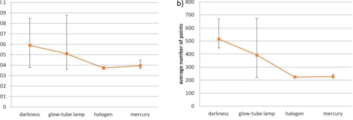
Fig. 3.3: Influence of the external lighting on the results, the whiskers represent max/min values ... 30

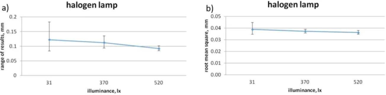
Fig. 3.4: Halogen lamp: a) range of results, b) RMS error, the whiskers represent max/min values ... 31

Fig. 3.5: The number of measurement points for the halogen lamp - different powers, the whiskers represent max/min values ... 31

Fig. 3.6: Measuring strategies: a) parallel, b) cross, c) chaotic [46] ... 32

Fig. 3.7: Sample standards of roughness ... 34

Fig. 3.8: Straightness of cross-sections for reflective surfaces ... 36

Fig. 3.9: Straightness of cross-sections for scattering surfaces ... 37

Fig. 4.1: General idea of data fusion method ... 39

(12)

Fig. 4.3: Different materials of ceramic balls: a) silicon nitride, b) tungsten carbide, c) zirconium

oxide, d) aluminium oxide ... 41

Fig. 4.4: Sphericity error for different diameters [44] ... 43

Fig. 4.5: Determination of ball's position [44] ... 44

Fig. 4.6: Metal sleeve for material markers ... 45

Fig. 4.7: Material markers ... 45

Fig. 4.8: Ball's data coverage (2D view) ... 46

Fig. 4.9: Artefact with material markers ... 47

Fig. 4.10: Measuring strategies: a) single scan, b) perpendicular scans, c) chaotic scan, d) single scan with intensive work of joints, e) high coverage scan [41] ... 48

Fig. 4.11: 3D and 2D deviation diagrams for strategies: a) single scan, b) perpendicular scans, c) chaotic scan, d) single scan with intensive work of joints, e) high coverage scan [41] ... 49

Fig. 4.12: Flowchart of virtual markers method [48] ... 51

Fig. 4.13: Determination of a characteristic point pair: a) • - point cloud from laser scanner, • - point from the CMM; b) determination of virtual sphere around the point from the CMM; c) selection of points inside the sphere (•); d) average of points from inside the sphere • - characteristic point, corresponding to the point from the CMM (•) [48] ... 52

Fig. 4.14: Pairs of corresponding points ... 53

Fig. 4.15: Inverse-variance weighting method for a pair of points ... 54

Fig. 4.16: Concept of correcting vectors [47] ... 55

Fig. 4.17: Test on different methods of weight determination ... 56

Fig. 4.18: Reliability function ... 60

Fig. 4.19: Research on λ determination on the example of a line ... 61

Fig. 4.20: Research on λ determination on the example of an arc ... 63

Fig. 4.21: Data fusion for a line - different density of markers ... 66

(13)

Fig. 4.23: Data fusion with uncertainties of characteristic points ... 71

Fig. 4.24: Results of data fusion taking expanded uncertainty into account ... 72

Fig. 4.25: The cube with material markers [47] ... 77

Fig. 4.26: Turbine blade with material markers [47] ... 78

Fig. 4.27: Engine cover with material markers [47] ... 80

Fig. 4.28: Planar test part. White markers are used for self-positioning. They enable to determine scanner’s relative position to the part [48] ... 82

Fig. 4.29: Principle of CMM measurements of the part (the actual number of points varies for different part geometry). • - reference data for evaluation of the method, • - characteristic points used for data fusion [48] ... 83

Fig. 4.30: Comparison between data from a CMM and a point cloud [48] ... 83

Fig. 4.31: Turbine blade with the 3CB for referencing [48] ... 85

Fig. 4.32: Comparison of cross-sections of point clouds before and after fusion with reference data [48] ... 86

Fig. 4.33: Engine cover with the 3CB [48] ... 87

Fig. 4.34: Measurand – plane part ... 89

Fig. 4.35: Distances between point cloud from non-contact measurement and reference data before data fusion ... 91

Fig. 4.36: Distances between point cloud from non-contact measurement and reference data after data fusion ... 91

Fig. 4.37: Cross section of a point cloud - plane part ... 92

Fig. 4.38: The magnified edge from Fig. 4.38 ... 93

Fig. 4.39: The curve characterization using characteristic points from contact method ... 94

Fig. 4.40: Comparison of cross-sections before and after data fusion ... 95

(14)

LIST OF SYMBOLS AND ABBREVIATIONS

3D_dev tridimensional centre deviation; a signal peak on the CCD array;

b systematic error;

B_i,p(u), Bj,q(v) normalized B-splines of degree p and q for the u and v directions;

C constant;

Cor_vect_j correction vectors;

d triangulation base;

dist distance between characteristic points;

dist_after mean distance after application of the ICP algorithm; distbefore mean distance before application of the algorithm;

D_i _{distances from each characteristic point to the points from the cloud;} E alignment error in the ICP algorithm;

f focal length;

F rigid transformation function; k number of pair points;

K coverage factor;

m mean time between failures;

max. dev. maximal difference between position from contact and non-contact measurement;

mean of dev. mean difference between position from contact and non-contact measurement; min. dev. minimal difference between position from contact and non-contact

measurement;

(15)

N number of measurements for weighted average calculation; pi, qi point-pairs from moving and fixed mesh respectively; pij jth measurement coordinate on the ith surface patch; Pa_f position of a point from the point cloud after fusion; P_AVE weighted average position calculated from P_CMM and P_LS; P_{b_f} position of a point from the point cloud before fusion; P_CMM position of characteristic point from LDHP method; P_LS position of characteristic point from HDLP method; q_ij corresponding nearest point to p_ij;

r(x) vector of the correlation values between the predicted point x and all points of the design of experiments;

ratioimp ratio of improvement;

R distance between optical centre and measured surface; R_m rotation matrix;

Re(t) reliability function;

R_θ correlation matrix of the design points; s(u, v) B-spline function;

t time;

t_m translation matrix;

T matrix for rigid body transformation; u(x) uncertainty of x;

U expanded uncertainty;

wi weights to calculate weighted average; Vc_i correcting vectors at characteristic points;

(16)

x any predicted point;

xavg weighted average of N measurements;

xij, yij, zij coordinates of the B-spline surface control points ϕij;

y corresponding response at points belonging or not to the designed experiment; σ_a uncertainty of the photodetector array;

σ_ave uncertainty of the weighted average; σ_i2 variance of ith measurement;

σ_R uncertainty of distance between optical centre and measured surface; σ_x, σ_y, σ_z standard deviations of position determination for each direction; n_u, n_v number of control points in the u and v directions in B-spline function;

θ incident angle;

λ sole distribution parameter; μ_ŷ(x) prediction value;

(17)

LIST OF APPENDICES

Appendix A – THE SPECIFICATION OF LEGEX 9106 ... 112

Appendix B – THE SPECIFICATION OF ACCURA 7 ... 113

Appendix C – THE SPECIFICATION OF REVSCAN ... 114

(18)

CHAPTER 1 INTRODUCTION

In contrast to conventional metrology, coordinate measuring techniques rely on computer processing of point coordinates gathered on the part surface. These points are used to characterise measured surface or feature. When large number of points are measured more complex information about the measurand is provided.

Points can be collected using contact and non-contact sensors. In the case of contact measurements high precision coordinates are obtained. The main disadvantages of this approach are the small number of measurement points and the long measuring time. Industry seeks faster and more thorough inspection of machined parts in order to shorten product process development time. An attractive solution is applying non-contact methods where much data of the whole object is gathered in a short time albeit with lower precision.

Unfortunately, every method has its advantages and disadvantages. The complexity and requirements of modern products means that it is often desirable to combine data from two measuring techniques. Therefore, in my dissertation I elaborated a method which allows combining two sets of data, maintaining the advantages and minimizing disadvantages.

1.1 Description of the problem

Results from the measuring process represent the true value of the inspected diameter with some level of uncertainty. It is caused by accuracy of the used, environmental conditions, measuring process etc. Results are burdened with two types of errors: random, which are unpredictable and systematic which are repeatable.

In coordinate metrology there are two methods of points collection: contact and non-contact. Contact measurement provides high accuracy data but density of points is low. Non-contact measurements are less accurate than contact measurements due to the presence of both systematic and random errors. But measurement data covers the inspected part with high density point cloud. Properties of both methods of points collection are presented in Fig. 1.1.

(19)

Fig. 1.1: Contact and non-contact measurements of a curve

As we can see from Fig. 1.1 measurement performed only in a non-contact way is characterized by high inaccuracy. Points from contact measurement are characterized by high accuracy, whereas a small number of points can make that the information deduced from them does not represent the actual state.

Inaccuracy of a measurement, which is much more significant in case of non-contact measurements, is caused by both systematic and random errors. Random errors are represented as noise in point cloud from non-contact measurement. Systematic errors are caused by measuring process and the non-contact device and increase the total inaccuracy of results.

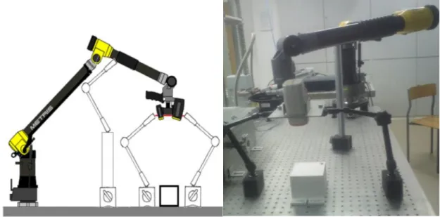
As sample devices to present coexistence of measuring errors a measuring arm and a CT scanner were used. Below it is shown, how systematic errors affect the results.

The first system is a coordinate measuring arm equipped with a laser scanner. In [45] the effect of the measuring strategy on the measuring results was described. Five different measuring strategies were chosen (marks of the axes are presented in Fig. 1.2 (5)).

1) The rotary axes (“A”, “C”, “E”, “G”) were immobile, only tiltable axes (“B”, “D”, “F”) were used in the process of data acquisition.

2) Axis “A” was rotated by 180°, during the measurement only tiltable axes were moved.

3) Axes “A” and “G” were rotated by 180°, during the measurement only tiltable axes were moved.

4) The rotary axes were immobile, only tiltable axes were moved but the surface was measured three times in the row.

5) Movement in all seven axes.

The first strategy is the simplest one and can be used in a very limited number of cases, where a part can be measured with a single scanning path without employment of rotary axes. In the

actual curve

points from contact measurements points from non-contact measurements shape deduced from contact measurement

(20)

second and third strategies before the measuring process one or two axes respectively were rotated by 180° but during the measurement their positions were not changed. In the fourth strategy the same surface was measured three times so individual scans overlapped. In many situations in real measurements it is impossible to avoid overlapping of scans which might be caused by the complex shape of the surface or unsuitable properties for optical measurements. The last strategy represents the situation in which big parts with quite complex shape are measured. Then all joints are rotated to cover the part with a laser beam.

These strategies are presented in Fig. 1.2

Fig. 1.2: Measuring strategies

Using these strategies a planar surface was measured and cross-sections of the resulting point clouds were analysed. The cross-sections are presented in Fig. 1.3.

(21)

Fig. 1.3: Cross-sections of point clouds along the scanning direction for all strategies As can be seen from Fig. 1.3 results from a measurement using measuring arm equipped with a laser scanner are burdened with two types of errors: systematic and apparently, random. In Fig. 1.3 both types are visible and appear with the same order of magnitude. In Fig. 1.3a systematic error is marked with a black line. As it can be seen the value of systematic error is around 160 µm while random error is up to 40 µm. It means that systematic errors are the main component of the total error.

Another example in which a non-contact measurement provides systematic errors is computed tomography (CT). In computed tomography the part is placed on a rotary table and X-rayed by beam in the form of a line or a cone. Then for each rotation position of the part its 2D image is collected by the detector. From all images the data is processed to create 3D volume rendering of the part. The results depend on many factors. Important factors are: proper positioning of the part on rotary table, set voltage and current of the X-ray tube and also the algorithm used to detect the border between the material and the air.

To show how the CT measurement process introduces systematic errors affecting results the plano-parallel plate presented in Fig. 1.4 was used.

(22)

Fig. 1.4: Plano-parallel plate

The plate was measured on a CT scanner and an STL file of the outer surface was created as the internal structure is not an object of my concerns. Then the plate was calibrated on a coordinate measuring machine (CMM) using a high density of points. These points were used to create a CAD model of the plano-parallel plate.

The mesh of triangles (STL) was transformed to the coordinate system of the reference CAD model, created using CMM data, using best-fit algorithms.

Table 1.1 presents geometrical parameters of the used plano-parallel plate computed for CMM reference data and from CT measurement.

Table 1.1 : Geometrical parameters of the plano-parallel plate.

Characteristic Reference (CMM) CT measurement

distance between planes, mm

16.139 16.745

radius of the cylinder, mm 23.417 22.436

Table 1.1 shows how non-contact measurement differs from the reference. The distance between two planes is here defined as a mean value from two distances for two directions - between a plane and centre of gravity of the other plane. A plane is calculated by Gaussian fitting to the measured points while centre of gravity is calculated as average value of coordinates of all points.

(23)

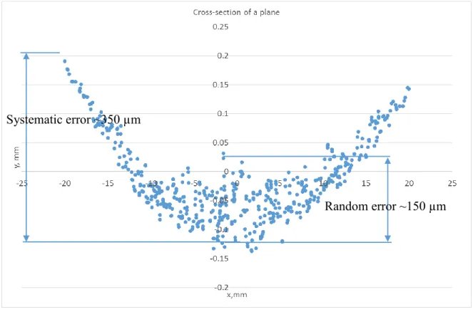
The radius has the value of Gauss cylinder fitted to data. For CT measurement this is about 0.6 mm higher while the radius is almost 1 mm lower, which shows that only scaling is not adequate. In order to present the nature of the distortion introduced by the measurement process a cross-section was extracted. It is presented in Fig. 1.5.

Fig. 1.5: Cross-section of CT data

As can be seen, results are affected by systematic and random errors. The cross-section should be linear, at that scale, while it appears concave. According to manufacturer specification flatness is of 63.3 nm which is negligible. When a line is fitted to this data using Gaussian method its position relative to the true value is incorrect. For this reason the measured height of the plate is also different from the reference. Fig. 1.6 shows a graphic comparison of the CT measurement minus the CAD model.

Systematic error ~350 µm

(24)

Fig. 1.6: Comparison between CT measurement and CAD model

As presented results showed, non-contact measurements introduce two types of error to the result – systematic and random. So why would not the operator use only contact method which are not susceptible to measurement conditions and provide more accurate data?

In almost all branches of industry, the production of parts requires thorough inspection of the first article and to some extent also every part made. Often, manufactured parts have to be assembled with others so their dimensions should conform to specific tolerances. Depending on the industry and function of the part, tolerances can have different values so inspection should be performed with proportional uncertainty.

On the other hand, measurement should be conducted as quickly as possible to decrease the total time and thereby the cost of the part production. Fast inspection is often contrary to the high accuracy measurement, which is time-consuming.

To solve this problem and to overcome limitations, an accurate and fast inspection method is needed. An idea is to combine data from two measuring methods that have different properties. The first method is accurate but rather slow. The second one is very quick but its accuracy is lower. Fusion of these two methods would provide high accuracy data in relatively short time. The contact measurement may be conducted only periodically if the non-contact method is found to have repeatable systematic errors.

Furthermore, time and costs of the measurements are not the only issues. There are some parts which cannot be measured using only contact methods. The sample part is a membrane keyboard

(25)

where areas around pads can be measured using contact methods while pads cannot. Their typical activation force is of 0.4 N. For example the pad would move during measurement with a TP20 Renishaw probe, which trigger force in Z direction is 0.75 N, and the measurement would be disrupted.

Another example is a traction network depicted in Fig. 1.7 for trams.

Fig. 1.7: Traction network

We can observe increase in the power of traction vehicles and an increase of their speed. This causes increase of technical requirements that traction network contact line must meet. Traction network must hang at a certain height. Too big a sag results in an incorrect cooperation between bow collector (pantograph) and the network which is particularly important at high speeds. Therefore, the height of traction network is controlled. Previously, it was measured using a contact measurement with special collector mounted on a traction vehicle but pressure on the traction line affects results. A recently developed method for this height control involves the use of vision systems. As it was shown non-contact methods provide two types of errors – systematic and random. Systematic errors can significantly change the results. In this case the use of two types of measurements, contact and non-contact, could also help. The whole traction network could be measured using the vision system and the result could be corrected using points gathered in contact way in places of network fastening – traction poles.

These examples showed that sometimes fusion of data from two measuring systems is a necessity not dictated solely by time or economic reasons. This makes the subject of data fusion relevant for research.

(26)

1.2 General objectives

The main objective of the present research is to fuse data of the same surface but obtained from different measuring methods. Some data may be derived from non-contact measurements like laser triangulation or structured-light projection technique and is characterized by a low precision but high density of points (HDLP). Other data may come from contact measurements and has low density of points but also higher precision (LDHP). The proposed approach is mainly suitable for freeform surfaces because in this case compensation of systematic errors is more complicated and standard methods cannot be used. The main goal is to increase the precision of one set of data, using the HDLP and LDHP sets.

1.3 Hypothesis

The precision of non-contact measurements can be increased by modelling point cloud on the basis of information from more accurate device. Using the proposed methods complex surfaces as well as simple ones with complex dimensions can be treated.

(27)

CHAPTER 2 LITERATURE REVIEW

2.1 Coordinate measuring technique

Coordinate measuring techniques are going through rapid developments thanks to the automation of measurements, the integration with CAD / CAM systems and the use of computer analysis and archiving of results. The first and still most common device used in coordinate metrology is the coordinate measuring machine (CMM). The accuracy of a CMM depends on the type of construction and on the measuring head. It is in the range of tens of microns, down to tenths of a micron. For part inspection two technologies can be used: contact and non-contact [27, 37]. In contact measurements high accuracy points from a surface are acquired by physical contact with the surface. The most obvious advantages are a lack of susceptibility to viewpoint or lighting conditions and an ability to inspect regions that cannot be reached by light beam. Another advantage is that CMM equipped with a contact probe can be used to extract features information from a small number of points [26]. The disadvantages are slower measuring speed than in case of non-contact measurements, limitations in the size of the part and the necessity to fasten the measured object [33], which is particularly significant for freeform surfaces [7] and big parts, which require much surface coverage and mechanical motion respectively. Note that when measuring a part with a CMM there are different sources of error like machine and part errors but also triggering probe and probe tip errors [39] . And also there are many factors affecting accuracy of touch trigger probes. Some of them were analysed in [64].

It is worth noticing that the set of measured points only constitute a small sample of the measured feature or surface. For this reason the quality and quantity of information obtained from a CMM depend on the number and distribution of measuring points [34]. Also as CMM software does not detect discontinued areas some information can be lost [63]. There is a need to find a compromise between the number of measuring points and measuring time. From an economic point of view the smallest sample should be chosen, but form errors require finding the maximum values of form deviations from a full-field inspection [40]. Depending on the task, point acquisition by CMM can be conducted in point-to-point and continuous scanning ways [37]. When points are collected in continuous mode, the density of points for a given time is higher, but so is uncertainty [62].

(28)

Nowadays faster and more thorough inspection of machined parts in order to shorten product development and production time is requested. An attractive solution is applying optical methods where data from the whole object is gathered in a short time. Unfortunately in optical methods larger uncertainty of points appears that reduces the benefit from higher density of points [37]. Optical methods include: triangulation, ranging, interferometry, structured lighting and image analysis.

A short comparison of contact and non-contact measuring methods was presented in the following subchapter.

2.2 Contact versus non-contact measurements

Both contact and non-contact measuring systems have their pros and cons. Contact systems give accurate data. Moreover scanning and routine operations can be repeated by using created measuring programmes. On the other hand, programming of measurement for complex components is tedious and the digitization is time-consuming. Non-contact scanning is fast and generates high density point cloud but resolution is limited and noise appears. Large memory is required to process the data [27].

In order to compare data from contact and non-contact measurements, both should be put into the same coordinate system. A common method of alignment is the use of three spheres located in the measuring space. They are measured together with the inspected part by all sensors. Then relation between centres of balls from different systems is calculated. Subsequently rotation and translation matrices are computed to minimize distances between these points [27]. To improve this kind of matching, spheres should have high diameters and should be as far as possible from each other [37]. There are also other methods to align part in the coordinate system. They are described below.

2.3 Part in the coordinate system

As in the process of measurement, the important issue is the location of the measuring part. There are a number of methods to define the position of the part in the coordinate system of the measuring device. The first type of alignment is by using some initial points and then by minimizing distances between measured and design points. This method is often called Best Fit Alignment. Another solution is the 3-2-1 approach where six points on three mutually

(29)

perpendicular planes are measured [51, 52]. Alas this method is only applicable for parts with plane surfaces [38]. There is also a method similar to the first one but where features are used instead of points. For the location of part in the measuring space dedicated tools and features can be used [38].

There are some problems with CAD-directed dimensional measurements. The first one is that actual measured point can be different from the intended ones. This is because of the lack of knowledge about the exact transformation between the device and the measured object and also due to dimensional errors of the part [38]. Uncertainty of the part’s localization is small relative to the size of the part, but more than one order of magnitude than the tolerances allowed by the manufacturing operation [21].

When the part is correctly localized in the measuring volume measuring plan shall be created. The process is described in the following subchapter.

2.4 Measuring plan

A serious limitation in coordinate measurements is the need for skilled workers to prepare the measuring plan. When defining the measurement plan, a basic problem is the selection of the number and location of the measuring points. The three most common methods are blind sampling: uniform sampling (not efficient, especially when small number of points is measured), Latin Hypercube Sampling (uniform projection of the samples on each of the axis of the hyperplane) and Hammersley sequence (compared to the first method, this approach gives a pleasant, less clumped pattern) [14]. The measuring plan is crucial to avoid false conformity positives [1].

In order to design the measuring plan, two kinds of information can be used: a priori information from the machining process or measurement of similar part and in-process information called adaptive measuring plan [40, 1].

There are three factors important in the process of optimization a sampling plan: time, accuracy and completeness of the measurement. For economic reasons, the number of measuring points should be limited but it is highly probable that a small number of points cannot adequately represent the inspected feature [15].

(30)

For contact measurements, a sampling strategy presented by Colosimo et al. in [9] can be chosen. The authors suggested choosing measuring points in the areas, where according to the construction requirements, deviation from the nominal value is the most important. This reduces the time and the cost of the measurement while providing crucial information.

For freeform surfaces, because it is not always clear where control points should be located, the conventional method is to create a grid of measuring points on 2D plane and project it on the surface. Subsequently, the obtained structure/pattern or only nodes of the grid are measured with the CMM. The disadvantage of this approach is that it is not relevant for complex shapes [33]. Also the best strategies for optical measurements were analysed. A procedure was presented for creating automatic scanning plan. First, an initial plan is generated and tested. Then it is verified whether all points can be measured with this initial plan and then if necessary, it is modified. Next, on the basis of critical points, scan directions and paths are generated. Finally, depth of field and occlusions are checked [32].

Another approach was presented by Seokbae et al. in [51]. At the beginning, a complex part is divided into some functional surfaces. This is performed on the basis of distances between critical points obtained from the initial scanning. The existence of critical points simply means that the surface on which they appear cannot be measured by a single pass of the scanner. Distances between these points are longer than the length of the laser stripe or the angles between their normal vectors are bigger than doubled the view angle. After these operations a scan path is generated. Finally, depth of field and occlusions are checked. This way, scan directions can be modified or added to generate a final scan path.

When a laser scanning plan is generated, a few constraints need to be satisfied. The first one is the angle between the surface normal and incident laser beam called view angle. It should be less than the value set for a given sensor. The part should also be within the length of the stripe generated by the laser emitter. Measured points need to be on a certain range of distance from the laser source. Determination of the measuring plan should take into account the lack of interference with the measurand and proper preparation of the surface being measured [66]. As was mentioned earlier, from the engineering point of view the number of measuring points should be limited [40]. This speeds up the inspection time of the part.

(31)

Edgeworth et al. [15] presented the iterative sampling method to determine a measuring plan on the basis of surface normal measurements. To this end, deviations of points’ location and surface normal from the nominal values were used. Afterwards, they created interpolating curves to predict the form error appearing between pairs of measuring points. This curve allows deciding whether the next measuring points are required to complete, within desired confidence limits, the measurement and selecting locations for the next sample. Their algorithm can also be used to identify outliers in a scanned surface data, because outliers can affect significantly the accuracy of the measurement. The limitation of this method is the necessity of having the nominal geometry which prevents its use, for example, in reverse engineering.

To create an adaptive measuring plan a curvature-based approach can be adapted. In this strategy points are concentrated in the areas with higher curvature [60].

Recently, to automate the measuring plan Kriging model began to be used. This model was developed based on works of G. Krige and initially used in mining. Kriging model allows interpolating the response at any location. This is performed by having design of experiment, where stochastic parameters are defined. Prediction value μŷ(x) can be expressed by the equation [14]:

𝜇𝑦̂(𝑥) = 𝛽 + 𝑟(𝑥)𝑅𝜃−1(𝑦 − 𝛽1) 2.1

where x is any predicted point, y is a corresponding response at points belonging or not to the designed experiment, r(x) is a vector of the correlation values between the predicted point x and all points of the design of experiments and R_θ is the correlation matrix of the design points, β is a set of coefficients. Basically Kriging model is used to iteratively update a measuring plan [40]. In [14] authors presented a strategy for adaptive inspection of parts to limit the number of measuring points. Their method can be adapted for big freeform surfaces, which makes it useful in various industries. The procedure starts with the measurement of initial points which are determined by the Hammersley sequence. Then, first a Kriging model is built. The model allows for iterative addition of points to the design of the experiment. Points are chosen on the areas at risk. The loop is ended when probability of the surface conformity is not smaller than a required confidence interval. Authors tested their algorithm for big parts from the aeronautic industry like: forward pressure bulkhead, upper part of a cockpit and landing gear compartment. Similar

(32)

approaches were presented also in [40] and [1]. Unfortunately, it is still time-consuming contact inspection.

Based on developed measuring plan the inspection is performed using selected measuring method.

2.5 Triangulation scanning

As it was mentioned there are few non-contact measuring methods. They include: triangulation, ranging, interferometry, structured lighting and image analysis. In my dissertation I focused mainly on laser scanners based on triangulation because of their broad use in industry. Triangulation scanners are more accurate and cheaper [37] than other non-contact measuring techniques and are faster than tactile methods [57]. Regrettably the uncertainty of laser scanners results is one order of magnitude higher than for contact probes [17]. The working principle of triangulation is as follows. A laser plane is sent by the transmitter to the measured part. The illumination by the laser of the inspected surface is observed by a CCD (charge-coupled device) camera. This gives 2D coordinates of points that are the intersection of the laser beam and the measured surface. The distance between optical centre and measured surface can be calculated from following equation [36]:

𝑅 = 𝑓𝑑_𝑎 𝑐𝑜𝑠 𝜃 + 𝑑 𝑠𝑖𝑛 𝜃 2.2

where f is the focal length, d is the triangulation base, a is the signal peak on the CCD array and θ is the incident angle. The geometric dependencies are presented in Fig. 2.1.

(33)

The uncertainty can be computed from the above equation and not including external factors (apart from incident angle) like for instance environmental conditions [36]:

𝜎_𝑅 ≈_𝑓𝑑𝑅2𝜎_𝑎 2.3

where σ_a is the uncertainty of the photodetector array.

For the uncertainty calculation, the use of a sensor precision as a sensor accuracy is common and accurate if the variance of the sensor does not change around the measuring range, as it is most influencing factor [36].

The third coordinate value is determined on the basis of the position of the scanner in determined coordinate system or in the coordinate system of the device moving the scanner [11, 57, 18]. Apart from advantages of laser scanning like high speed, high-resolution and non-contact sensing, this method has also some limitations. There are many factors affecting laser scanning accuracy. The most important seems to be the properties of the measured surface like reflection, chemical composition of the material, microstructure and roughness. The best measurement results can be obtained with surfaces that produce a good diffuse reflection at the same wavelength as the laser source [57]. Therefore, a special preparation of the part is necessary in some instances. For example specular or transparent surfaces should be covered for example with special layers [57, 51] of white powder. Moreover geometric obstruction, like relative position between the sensor and the measured surface can affect laser scanning measurement [57, 61, 49]. Ultimately, the combined effects of environment, operation error, data processing, fitting and transformation error must be considered [61].

There are two main strategies when laser scanning is conducted. The first is a global strategy where orientation changes of the scanner during the measurement are minimized. In the second one, called multi-oriented strategy, the laser scanner passing over the surface is swivelling to maintain the laser beam normal to the surface during the entire measurement. However, it was proved that differences between both strategies are insignificant [37].

The most important disadvantage of optical measurements seem to be the lack of knowledge about the measurement uncertainty [37] and how to determine the best methodology for the measurement. To this end, factors affecting the accuracy of laser scanning were widely analysed and discussed by many authors.

(34)

In [12] it was shown that when the laser beam is perpendicular to the surface the highest number of points is acquired. Equally important are the distance between the surface and the device and the angle between the laser beam and the normal vector to the surface. A higher resolution is obtained when the sensor is close to the measured surface [57] and at small incident angles [59]. It was also showed that the intensity of the laser should be specified according to the surface colour, shape and roughness. Concerning the surface colour, for most common lasers with red colour of the beam, the best results are obtained for red surface, then for green and blue respectively [58]. Experimental equation used to calculate number of acquired points according to sensor-to-surface distance, longitudinal angle of measurement and relative reflection rate of the measured surface can be determined and then used to correct the measurement [58].

It is important to acquire points over the entire surface. It seems to be obvious that if fewer points are acquired, the quality of scanning is poorer. Additionally, gaps appear in the data that need to be filled by mathematical calculations on the basis of existing points. Moreover, filling gaps is performed according to user-defined parameters. This results in an unknown error.

Concerning illumination conditions, measurements should be conducted in the absence of external light. Although the best results are obtained with the absence of light, this approach is not convenient for many measuring tasks. For this reason often mercury vapour lamps (MVL) are used. This solution is better than halogen illumination regardless of the material of the measured part [3].

In [11] it was presented that errors in laser scanning are caused by two main sources. First is the influence of the laser interaction with the surface. Second are defects and distortions caused by the lenses.

2.6 Registration process

Results of laser triangulation measurement can be strongly affected by improper registration process. For instance, for large parts or objects with complex geometry it is impossible to measure the whole part with a single pass of the scanner. This is another inconvenience in triangulation based measurements.

An important issue in the registration process is that, all scans from different viewpoints need to be transformed into a common coordinate system [20].

(35)

There are different approaches to perform this task. The simplest approach seems to be the use of three coordinate balls (3CB) to calculate relations between paired merging views [26]. When using 3CB it is necessary to minimize obstruction of the part by the balls. In determination of rigid transformation following objective function is minimized [26]:

𝐹 = ∑ ∑ |𝑇−1_𝑝 𝑖𝑗− 𝑞𝑖𝑗|2 𝑚 𝑗=1 𝑛 𝑖=1 2.4

where T is the matrix for rigid body transformation, p_ij is the jth measurement coordinate on the ith surface patch, and q_ij is the corresponding nearest point.

Another approach to provide a common coordinate system was presented by Kuang-Chao et al. [30]. In their method first a set of data is considered as fixed and to this data a surface is fitted. The second set is mobile and is transformed to the frame of the first set. Then a blending area is selected and the minimization function is applied in this area.

2.7 Data processing

Data from 3D optical digitization are known to be noisy, inaccurate and presenting gaps. Authors in [31] suggested adding quality indicators like complete “κ” and accurate ”τ” to numerical representation of a point cloud. In previous works noisy “δ” and dense “ρ” indicators were listed. Noisy indicator δ is connected with sampling errors. Dense indicator ρ depends on user’s scan planning and as the name suggests specifies the density of a point cloud. The completeness shows the importance of existing gaps and the accuracy is a notion of uncertainty.

The common approach to reducing noise is the use of a median filter where point coordinates are replaced by the median values of sets of points from the closest neighbourhood. The drawback is that it is not appropriate for sharp edge features [27]. In a similar way, average filter is also used, but in this case the average value is used instead of the median.

Also very important is the removal of outliers before the fitting process because they can affect the alignment [50]. They do not belong to the measured surface and should not be treated as such.

2.8 Measuring accuracy

Some terms can be presented concerning the quality and utility of measurements. Accuracy is defined by how well the measuring point agrees with the point which is the intersection between

(36)

laser beam and the measured surface. Precision is a variation from sets of measurements from the same intersection point [36]. Measurement error is defined by the difference between measured and true values. Uncertainty is defined as follows: non-negative parameter characterizing the dispersion of the quantity values being attributed to a measurand, based on the information used [29]. Uncertainty, in simplification, can also be defined as a collection of all measurement errors [16].

Generally, measurement error can be divided into two categories: systematic and random. The systematic one has always the same value under the same measuring conditions and random error depends on factors affecting laser scanning [57]. In some cases systematic error can be predicted. Ratio between random and systematic error should be small [17] so that compensation of systematic error will give desirable results.

Concerning errors in a laser scanning, it was noticed that, when the projected angle is around 0o the random error is the highest but when projected angle increases the systematic error increases. When scan depth is larger the influence of the projected angle is smaller [17].

A method intended to separate systematic from random error was presented in [56]. To this end a reference plane was measured with different scan depth. The distances between planes were considered to be systematic errors as a function of scanning depth and standard deviation on one plane indicated random error.

2.9 Error compensation of laser scanning and system calibration

In order to overcome the accuracy limitations of laser scanning, attempts to compensate the error were made.

In [5] Bracun et al. presented tests results of a one-shot triangulation system. They measured a surface illuminated by a number of light sheets and observed that the curvature of the stripe increases for stripes further from the central one.

Xi et al. [65] presented a method for laser scanner’s error compensation. For this purpose an artefact composed of a ball fastened at a constant distance from a reference plane was used. They observed that measurement error, calculated from the distance between the centre of the ball and the plane, depends on angle and scan depth so an empirical formula for error estimation was determined and used to compensate the errors in actual measurements.

(37)

Common approach to calibrate vision systems uses the tip of a CMM probe as a target. The positions of the tip, from optical measurement are determined in various locations in space and are compared with positions indicated by the readout system of the CMM. The ball is used because its view is circular from all angles and its centre position can be calculated easily [52]. A similar approach is also presented in [58].

Santolaria et al. [49] presented another method for camera calibration. For this purpose they created an artefact in the form of an artefact with a set of calibration points. Positions of points from optical measurement were compared with calibrated values and analysed for different positions and angles of the camera.

To obtain knowledge about the measuring error of a particular device, a quick verification test can be performed as in [56] in which a reference plane was measured for different positions and orientations of the laser scanner. Then, a least squares plane was fitted to all points. The fit residuals provide a value for the maximum expected measurement error.

2.10 Multisensory architectures and data fusion

Another approaches to overcome the accuracy limitations of non-contact measurements are multisensory architectures and data fusion. Multisensory architectures are applicable to reduce uncertainty, improve reliability, increase coverage or decrease measuring time. Sensors can be integrated in different ways: mounting of contact and optical probes in the same frame or one measurand can be inspected by separate devices [62, 50]. Sensors registration is necessary.

A classification of data fusion methods was presented by Boudjemaa et al. in [4]. Authors named four methods of fusion: fusion across sensors, fusion across attributes, fusion across domains and fusion across time (filtering). In fusion across sensors the same property is measured by different sensors. In fusion across attributes different quantities, but connected with the same experimental situation, are measured by different sensors. In fusion across domains the same attribute over various ranges or domains are measured by different sensors. Finally, fusion across time, merges new data with historical information.

Representation of data from different measurement methods in the same coordinate system was the impetus that has triggered the researches on methods of fusion of these measurements [50]. The purpose was to take the most appropriate information from each of the method. That

(38)

improves the quality and completeness of the measurement. On one hand accuracy of laser scanners is one order of magnitude less than for tactile probe and with much noise but on the other hand triangulation scanning yields data with high density in a short time. That is why recently, integration of contact and non-contact systems is gaining attention [61]. Data fusion may overcome the limitations and drawbacks of the individual sensors like for instance low speed of CMMs [34]. Also, sometimes single sensor cannot derive complete information about the object [62].

Several methods for data fusion were presented. Many authors proposed to use information from non-contact device to create a coarse CAD model of the measured object. Then having a priori knowledge about the part, inspection is performed by contact probe [62, 52, 8, 35]. It is particularly important when the CAD model of the measured object is not available [27].

A similar approach was presented by Carbone et al. in [7]. The integration method is at the level of aggregation of the information, not a physical integration. First, a vision system digitizes the physical object with a structured light scanner, with a mean error within 0.1mm. Then, data is ordered and filtered. After these operations in the CAD environment, curves are reconstructed and a rough model is created. This model has an accuracy of 0.5 mm which is sufficient to create a collision-free measuring path. The rough model is used for digitization and inspection of the part with a CMM. The first digitization Bezier surfaces are created. Finally the created Bezier surfaces are used to perform the inspection again, until the required reconstruction accuracy is achieved.

Freeform surfaces can also be represented by a few parametric equations like Coons patches, B-splines and NURBS (Non-Uniform Rational B-Splines). B-spline can be expressed by the following equation [34]:

𝑠(𝑢, 𝑣) = ∑ ∑𝑛𝑣−1𝐵_𝑖,𝑝(𝑢) ∙ 𝐵_𝑗,𝑞(𝑣) ∙ 𝜙_𝑖𝑗 𝑗=0

𝑛𝑢−1

𝑖=0 2.5

where: n_u, n_v are the number of control points in the u and v directions; ϕ_ij (i=0,1,…, 𝑛_𝑢−1, j=0,1,…, 𝑛_𝑣−1are the n (n=𝑛_𝑢 × 𝑛_𝑣) control points and B_i,p(u), B_j,q(v) are the normalized B-splines of degree p and q for the u and v directions respectively.

Measuring points with corresponding location parameters [uk,vk] can be represented by [34]:

𝑥_𝑘= ∑ ∑𝑛𝑣−1𝐵_𝑖,𝑝(𝑢_𝑘) ∙ 𝐵_𝑗,𝑞(𝑣_𝑘) ∙ 𝑥_𝑖𝑗 𝑗=0

𝑛𝑢−1

(39)

𝑦_𝑘 = ∑ ∑𝑛𝑣−1𝐵_𝑖,𝑝(𝑢_𝑘) ∙ 𝐵_𝑗,𝑞(𝑣_𝑘) ∙ 𝑦_𝑖𝑗 𝑗=0 𝑛𝑢−1 𝑖=0 2.7 𝑧_𝑘= ∑ ∑𝑛𝑣−1𝐵_𝑖,𝑝(𝑢_𝑘) ∙ 𝐵_𝑗,𝑞(𝑣_𝑘) ∙ 𝑧_𝑖𝑗 𝑗=0 𝑛𝑢−1 𝑖=0 2.8

where: xij, yij, zij are the coordinates of the B-spline surface control points ϕij.

In another approach for data fusion, during the measurement, large range devices are used first. Subsequently for specific features devices with smaller range but higher resolution are used. The objective is to limit measuring time. High-resolution measurements are applied only for a limited number of critical positions or features [62].

There are also methods [53, 54] in which data from non-contact sensor is used to determine a set of surface points that are re-measured in a tactile way.

A common approach is to measure the part with different devices and then replace features/surfaces which cannot be measured by one method by data from a more suitable one. For example, when a measured part has small cylindrical holes which cannot be measured by an optical system, the information about these features are obtained from contact measurement [62]. Another common approach to data fusion uses scanning of geometric surfaces with laser scanner and on measurement of accurate features by contact CMM. Then connection between both measurements is created [26]. For this case the mutual position of the sensors is calibrated [27]. For this purpose, calibration targets are used [52]. In [6] authors presented the most common method to calibrate integrated systems composed of CMM and laser scanner. In this method a ball is attached to the CMM’s table and is measured by both contact and optical probes. The drawback of this method is that it is accurate only if measurement is performed in the vicinity of the calibration position.

Another method for high- and low-resolution data fusion was presented by Jamshidi et al. in [27] and [26]. CMM and Laser Scanner (LS) data registration uses three balls. Then both sets of data are converted to IGES format. Subsequently, data from CMM are used to reduce the data from LS. If features scanned by CMM are in the neighbourhood of the same features from LS, the LS data, within a desired tolerance, are wiped out and replaced by their CMM’s equivalent. At the end, all features from contact measurement are attached to the mesh of triangles from optical measurement. Unfortunately their method can only be used to improve measurement of the part with precision features and is not suitable for freeform surfaces, as for research presented in [61].

(40)

There are also some commercial solutions for data fusion. One of them, called VAREA initially generates a triangular patch by the use of a vision system and then the digitization process is performed on a CMM. It cannot process freeform surfaces [34].

An interesting approach was presented in [55]. The authors proposed a method of data fusion from multi-resolution sensors. After measurement of a part using two types of devices features in both are detected. Then Points of Interest (POI) or Regions of Interest (ROI) are used to create the merged model. Points/regions from both methods that are closer to initial model are taken to create the merged model. Authors did not present how their algorithm would work for freeform surfaces without other features.

The subject of data fusion was also considered by Hannachi et al. [22]. In their approach the most accurate system reconstructs the outline of the object, while the less accurate one is used to characterize its 3D surfaces. In this approach distortions in measurements of the surfaces are not corrected.

Senin et al. in [50] used the ICP algorithm for data fusion. A point cloud from optical measurement is iteratively aligned to data from a CMM by finding corresponding points. They also augmented fixed point set to cope with the lack of point co-localization and so improved the registration result. The method requires having points arranged on a regular grid. Therefore as an optical measurement method only structured light scanning can be used. Triangulation laser scanners cannot be used because it is difficult to find specific point in the high density, unorganized point cloud that corresponds to point obtained with the use of CMM.

Colosimo et al. [10] proposed a method of data fusion via Gaussian models. This method uses kriging to predict the coordinates of points based on multiple measurements but putting different weights to data from different sensors.

2.11 Iterative closest point algorithm

In [27, 26] and [50] the merging process was performed by the use of the iterative closest point (ICP) algorithm, where points from overlapping areas are used to find transformation.

Generally in the ICP algorithm, an optimal transformation matrix to move one set of points relatively to another fixed point set is iteratively determined [50].

(41)

The ICP algorithm starts with two meshes between which the initial estimation of the rigid-body transformation is calculated. Subsequently, at each iteration the transformation is refined by the selection of new corresponding points in both meshes. Points are chosen from the overlapping areas. The best rotation and translation matrices are determined as to minimize the distance between both meshes [20, 19].

There are two approaches to the ICP algorithm: point-to-point (pt2pt) and point-to-plane (pt2pln). In the pt2pt algorithm, at each iteration, points from the moving set are associated with the closest points from the fixed set and transformation between corresponding points is calculated. In pt2pln algorithm instead of choosing a point from the fixed set, the new closest point is determined on the plane passing through the closest point from the fixed set. Authors proved that pt2pln gives better results [50].

The alignment error in the ICP algorithm is given by equation [19]: 𝐸 = ∑ ((𝑅_𝑚𝑝_𝑖 + 𝑡_𝑚− 𝑞_𝑖) ∙ 𝑛𝑖)

2 𝑘

𝑖=1 2.9

where (𝑅_𝑚, 𝑡_𝑚) are rotation and translation respectively, (pi, qi) are point-pairs from moving and fixed mesh respectively from set of k pairs, ni is a normal vector of plane passing through qi (taking into account the points from nearest neighbourhood).

The main disadvantage of the ICP algorithm is that errors from each scans are cumulated [26]. The transform is calculated based on overlapping areas so if points from this region are burdened with error, position of mobile cloud is not optimal. This is particularly visible in the case of a merger of multiple scans. Another limitation of the ICP algorithm is that some features/surfaces need more constraints. In vision systems this problem can be avoided by the use of other constraints, such as colour [19].

In general the ICP algorithm is not matched to the specific problem. It is rather treated as a black box where implementation is not optimized regarding the form of the data. Therefore some points from different datasets cannot be found in exactly the same position of the measurand [50]. To sum up, the most important advantages of the ICP algorithm include: no pre-processing of data and features extraction are required, independency on the shape representation and it is handling all of six degrees of freedom. The disadvantages are, that the ICP cannot be easily

(42)

adapted to the weighted least squares extensions, uncertainties of points can be different and the ICP algorithm is sensitive to outliers [2].

Variations of the ICP algorithm exist. In [23] IRF (iterative registration and fusion) and pure ICP algorithms were compared. The IRF consists of two steps. First ICP is used to register data from different sensors or viewpoints, and then a Kalman filter is used to fuse aligned data. The Kalman filter uses a series of measurements that contain noise to estimate unknown variables with higher precision. It was proved that the IRF algorithm is less affected by the number of measurements than ICP but requires an initial estimation of the underlying surface.

2.12 Frontier of knowledge

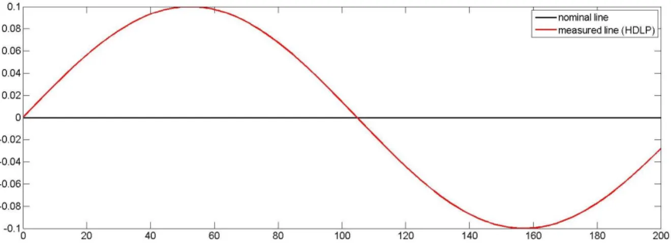
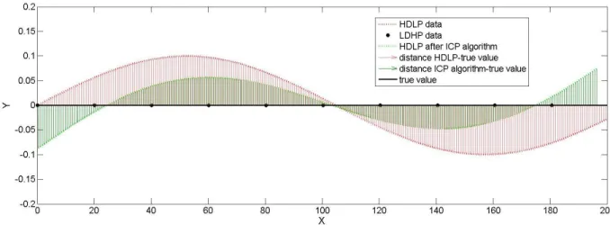
Recent method of data fusion [50] dedicated to freeform surfaces has many limitations. One is the requirement for the data to follow a regular grid. When data from non-contact measurement is aligned to the data from contact measurements, the dimensional errors of measuring points have a significant influence on the accuracy of this transform. Thus it is impossible to map one set of points exactly to another [33]. ICP algorithm is a rigid transformation and it is only about getting more precise alignment sensitive to noise. There is also no scaling. This means that relations between points do not change, the whole point cloud is treated as a single object. Therefore point cloud modelling is not complete and no real improvement is obtained.

To show how ICP works the following simulation was performed and is presented in Fig. 2.2.