UNIVERSITÉ DE MONTRÉAL
EFFICIENT LEARNING OF MARKOV BLANKET AND MARKOV BLANKET CLASSIFIER
SHUNKAI FU
DÉPARTEMENT DE GÉNIE INFORMATIQUE ET GÉNIE LOGICIEL ÉCOLE POLYTECHNIQUE DE MONTRÉAL
THÉSE PRÉSENTÉE EN VUE DE L‟OBTENTION DU DIPLÔME DE PHILOSOPHIAE DOCTOR
(GÉNIE INFORMATIQUE) AOÛT 2010
UNIVERSITÉ DE MONTRÉAL
ÉCOLE POLYTECHNIQUE DE MONTRÉAL
Cette thèse intitulée:
EFFICIENT LEARNING OF MARKOV BLANKET AND MARKOV BLANKET CLASSIFIER
présenté par : FU Shunkai
en vue de l‟obtention du diplôme de : Philosophiae Doctor a été dûment accepté par le jury d‟examen constitué de :
M. GAGNON Michel, Ph.D, président
M. DESMARAIS Michel ,Ph.D, membre et directeur de recherche M. PAL Christopher J., Ph.D, membre
DEDICATION
The author wishes to dedicate this dissertation to my family, who offered me unconditional love and support throughout the course of this thesis.
ACKNOWLEDGEMENTS
My utmost gratitude goes to my master and doctoral program supervisor, Dr. Michel C. Desmarais for bringing me to Ecole Polytechnique de Montreal, for his expertise, kindness, and most of all, for his patience. I believe that one of the main gains of this 5-year program was working with Dr. Michel C. Desmarais and gaining his trust and friendship. My thanks and appreciation goes to the thesis committee members, Dr. Michel Gagnon, Dr. Christopher Pal and Dr. Doina Precup. I do owe thanks to Dr. Wai-Tung Ho and Dr. Spisis Demire for their sharing and guide during my time in SPSS. Also, I thank my wife, Shan Huang who stands beside me and encourages me constantly. My thanks goes to my children, JingYi and JingYao for giving me happiness and joy. Finally, I would like to thank my parents whose love is boundless.
CONDENSÉ EN FRANÇAIS
Cette thèse porte sur deux sujets très reliés, à savoir la classification et la sélection de variables. La première contribution de la thèse consiste à développer un algorithme pour l'identification du sous-ensemble optimal de variables pour la classification d'une variable cible dans un cadre bayésien, sous-ensemble que l'on désigne par la Couverture de Markov d'une variable cible. L'algorithme développé, IPC-MB, affiche une performance prédictive et une complexité calculatoire se situant au niveau des meilleurs algorithmes existants. Cependant, il est toutefois le seul algorithme affichant les meilleures performances sur les deux plans simultanément, ce qui constitue une percée importante au plan pratique.
La Couverture de Markov d'une variable cible est un sous ensemble qui ne comporte pas de structure, notamment le réseau bayésien des variables impliquées. La seconde contribution consiste à exploiter les résultats intermédiaires de l'algorithme IPC-MB pour améliorer l'induction de la structure du réseau bayésien correspondant à la Couverture de Markov d'une variable cible. Nous démontrons empiriquement que l'algorithme pour induire la structure du réseau bayésien est légèrement plus efficace qu'un algorithme standard comme PC qui n'utilise pas les données intermédiaires de IPC-MB.
La sélection des variables pertinentes pour une tâche de classification est un problème fondamental en apprentissage machine. Il consiste à réduire la dimensionalité de l‟espace des solutions en éliminant les attributs qui ne sont pas pertinents, ou qui le sont peu. Pour la tâche classification, un jalon important vers la résolution de ce problème a été atteint par Koller et Sahami [1]. Basé sur les travaux de Pearl dans les réseaux bayésiens [2], il a établi que la Couverture de Markov (Markov Blanket) d‟une variable T représentait le sous-ensemble optimal d‟attributs pour la prédiction de sa classe. Nous le dénotons lorsque la variable cible est connue et par autrement.
Induire étant donné un réseau bayésien est un problème trivial. Cependant, l‟apprentissage de la structure d‟un réseau bayésien à partir de données est un problème reconnu comme NP difficile [3]. Pour un grand nombre de variables, l‟apprentissage d‟un réseau bayésien est en pratique très difficile non seulement à cause de la complexité calculatoire, mais aussi à cause de la quantité de données requises pour des problèmes dont la dimensionalité est très grande. Souvent, le problème de la dimensionalité est contourné en imposant des contraintes sur la
structure comme c‟est le cas avec les réseaux bayésiens naïfs [4, 5], qui sont probablement les plus répandus. Leur complexité calculatoire est relativement faible, n‟ayant pas à effectuer un apprentissage de la structure du réseau, et leur effacité est très souvent relativement bonne malgré les hypothèses fortes qu‟ils imposent.
Une des extensions des réseaux bayésiens naïfs est le formalisme de réseaux bayésiens naïf arborescent (Tree-Augmented Naïve Bayes, ou TAN) [6]. Les TAN sont généralement plus performants que les réseaux bayésiens naïfs en permettant certaines formes de dépendance parmi les attributs. Cependant, ils repondent néanmoins sur des hypothèses fortes qui peuvent les rendre invalides en général. Du fait que les réseaux bayésiens ne font pas d‟hypothèses fortes sur les données, on s‟attend que leur performance pour la classification soit meilleure que pour un réseau bayésien naïf ou un TAN [7]. Cependant, il faut noter que pour la tâche de classification, seulement un sous-ensemble du réseau bayésien est effectif pour la prédiction, c‟est-à-dire la Couverture de Markov du nœud cible, . Lorsque ce sous-ensemble est utilisé aux fins de classification, nous y référerons par , c‟est-à-dire le classificateur basé sur la Couverture de Markov. En général, le classificateur est considérablement plus petit que le réseau bayésien et sa performance est en théorie équivalente à celle du réseau bayésien complet. L‟induction de et sont deux problèmes très près l‟un de l‟autre, bien que l‟induction de peut s‟avérer être une étape indépendante.
Cette thèse aborde le problème de l‟efficacité de l‟apprentissage de et à partir d‟un échantillon de données limité. L‟objectif premier est de fournir un algorithme général de sélection des variables, ou attributs, tel que requis pour différentes tâches de classification, ou même de forage de données. Notre première contribution est de définir un algorithme qui élimine les attributs non pertinents d‟un (ou ) sous l‟hypothèse de la fidélité (voir plus loin), lorsque la Couverture de Markov d‟une variable cible T est unique et composée des parents de T , de ses enfants et de ses conjoints, ou spouses, [2]. Selon notre revue de la littérature, il existe au moins neuf travaux publiés depuis 1996 portant sur l‟apprentissage de la couverture de Markov, c'est-à-dire depuis que le concept a été démontré être le sous-ensemble optimal d‟attributs pour la prédiction et malgré le fait qu‟il est connu depuis 1988 [1][2].
Tous les algorithmes connus peuvent être regroupés en deux catégories : (1) ceux qui dépendent de la propriété d‟indépendance conditionnelle , où T est considéré indépendant de
toutes les autres variables étant donné les valeurs connues de ; et (2) les algorithmes qui reposent sur l‟information topologique, c‟est-à-dire la recherche des parents, enfants et conjoints du nœud cible. IAMB [8] est l‟exemple le plus représentatif des algorithmes du premier groupe. Sa complexité calculatoire et son implémentation sont toutes deux d‟une grande simplicité. IAMB comporte deux phases: la phase de croissance et celle de décroissance. Chaque phase nécessite la vérification de savoir si une variable X est indépendante de T étant donné un ensemble de nœuds candidats de la Couverutre de Markov, , puis d‟enlever ou d‟ajouter des nœuds de cet ensemble de candidats. PCMB [9] est la contribution la plus récente aux algorithmes avant nos travaux et il est un exemple du second groupe. Ce fut en réalité le premier et alors le seul algorithme dont la preuve a été faite qu‟il peut induire la Couverture de Markov, bien que ce n‟est toutefois pas le seul qui s‟est appuyé sur l‟information topologique pour le faire. Malgré ces avancements, la recherche d‟un algorithme qui peut à la fois garantir de recouvrer la Couverture de Markov et le faire en un temps raisonnable et avec un ensemble de données réaliste demeure un objectif non atteint. Par exemple, KS [1] est un algorithme approximatif (il ne peut garantir de recouvrer la Couverture de Markov); IAMB est un algorithme simple qui peut fournir cette garantie, mais il impose une quantité extraordinaire de données afin d‟arriver à un résultat acceptable pour des problèmes pratiques; MMPC/MB [10] et HITON-PC/MB [11] représentent les premiers essais pour améliorer l‟efficacité en regard des données par l‟exploitation de données topologiques, mais il a été démontré qu‟ils n‟offrent pas la garantie de recouvrer la Couverture de Markov [9]; PCMB a suivi la découverte de MMPC/MB et de HITON-PC/MB, et ils peuvent effectivement fournir de bien meilleurs résultats que IAMB pour les mêmes données. Cependant, PCMB est beaucoup plus lent que IAMB, et nos résultats suggèrent même qu‟il peut nécessiter plus de temps que l‟algorithme PC (voir Chapitre 4). Nous proposons l‟algorithme IPC-MB [12-14] afin d‟offrir une solution qui vise à la fois à fournir des résultats en un temps rapide et avec une quantité de données réaliste. Cet algorithme est de la seconde catégorie, c‟est-à-dire qu‟il utilise l‟information topologique pour dériver la couverture de Markov.
Tout comme les algorithmes MMPC/MB [10], HITON-PC/MB [11] et PCMB, l‟algorithme IPC-MB divise l‟apprentissage de en deux phases séparées, l‟induction de et de . Dans la première phase, IPC-MB effectue une recherche pour trouver les voisins immédiats du nœud et elle est commune aux algorithmes PCMB, MMPC/MB et HITON-PC/MB. Cependant, alors que
ces algorithmes effectuent une série de tests afin de déterminer si un nœud X n‟est PAS indépendant du nœud cible T étant donné tous les ensembles possibles de conditions, c‟est-à-dire où , IPC-MB présume initialement que toutes les variables du domaine à l‟exclusion de T (c.-à-d. \{T}) sont des candidats à . Puis, l‟algorithme élimine les variables une à une si X est indépendant de T étant donné un ensemble de conditions quelconque. Parce que la majorité des réseaux ne sont pas denses en pratique et que IPC-MB commence par des ensembles conditionnels vides pour les élargir un nœud à la fois, il lui est possible d‟éliminer la majorité des faux candidats avec un petit ensemble de conditionnels, ce qui entraîne un gain en termes de calculs et de données nécessaires. Bien que certains descendants de
T peuvent demeuré dans , ils sont rapidement éliminés en réexecutant la même recherche pour chaque (candidats de qui est le résultat de la recherche précédente) afin de déterminer si . De plus, en reconnaissant que tous les conjoints sont contenus dans l‟union des résultats des recherches pour , c.-à-d. , et que seulement les véritables conjoints contenus dans seront dépendant de T conditionnellement à l‟ensemble séparateur trouvé précédemment plus X, une quantité importante de ressources est économisée en comparaison avec PCMB afin de dériver .
Nous faisons la preuve que l‟algorithme IPC-MB est valide et comparons sa performance avec les algorithmes qui sont actuellement l‟état de l‟art, notamment [10], PCMB [9] et PC [15]. Les expériences effectuées avec des échantillons de données générées à partir de réseaux bayésiens connus, notamment des réseaux de petites tailles comme Asia qui compte huit nœuds, des réseaux moyenne envergure comme Alarm et PolyAlarm (une version polyarborescence, polytee, de Alarm) avec 37 nœuds, et des réseaux plus grands comme Hailfinder (56 nœuds) et Test152 (152 nœuds). Nous mesurons la performance des algorithmes en termes de précision, rappel et de distance ( ). Le temps de calcul est mesuré en termes de nombre de tests d‟indépendance conditionnelle (CI) et de nombre de passes qui doivent être effectuées sur les données (relectures des données), car une seule passe n‟est généralement pas suffisante pour mettre en cache toutes les fréquences requises en mémoire. Ces mesures sont couramment utilisées, car elles sont indépendantes du matériel utilisé et représentent la grande partie des ressources calculatoires consommées pour ce type d‟algorithmes.
Les résultats démontrent que, IPC-MB fournit (1) un niveau de performance nettement supérieur à IAMB pour une quantité d‟observations équivalente, atteignant jusqu‟à 80% en réduction de distance (mesurée par rapport au résultat idéal), (2) a une performance légèrement supérieure à PCMB et PC (toujours à quantité de données égales), (3) nécessite jusqu‟à 98% moins de tests CI que PC et 95% moins que PCMB, et (4) en moyenne les tests CI comportent un ensemble conditionnel relativement plus petit par rapport à IAMB et PCMB (ce qui est en bonne partie à la source des améliorations observées). Nous pouvons donc conclure que les stratégies d‟apprentissage de et adpotées pour IPC-MB sont très efficaces et permettent un gain significatif pour atteindre l‟objectif d‟induire la Couverture de Markov avec un rapport réaliste de temps et de données.
Étant donné le résultat de IPC-MB, c.-à-d. , les algorithmes conventionnels pour induire la structure d‟un réseau bayésien peuvent être appliqués pour recouvrir autre modification puisque l‟apprentissage de est indépendant d‟eux. La complexité de l‟apprentissage de la structure devrait être considérablement réduite en comparaison de l‟apprentissage induit de l‟ensemble des variables du domaine . Nous avons réalisé une autre étude dans le cadre de la thèse en appliquant l‟algorithme PC pour l‟apprentissage de la structure étant donné , l‟algorithme IPC-MB+PC, et avons observé un temps de calcul considérablement réduit. En fait, le résultat de IPC-MB peut être considéré comme la sélection de variables d‟un problème et être utilisé dans un grand nombre d‟algorithmes de prédiction. L‟algorithme a d‟ailleurs été développé par l‟auteur lorsqu‟à l‟emploi de SPSS en 2007 et il est actuellement intégré au module Clémentine 12 pour dériver un .
Une seconde contribution de cette thèse est l‟extension de IPC-MB pour induire la structure d‟un directement sans avoir à dériver l‟ensemble du réseau bayésien au préalable comme la solution IPC-MB+PC le fait, ce qui constitue une première à notre connaissance. Cet algorithme est nommé IPC-MBC (ou IPC-BNC dans une publication antérieure) [16]. Tout comme IPC-MB, il repose sur une recherche locale afin de déterminer les voisins d‟une variable.
Étant donné une variable cible , l‟algorithme IPC-MBC peut être divisé en 5 étapes, après une initialisation où le nœud T est assigné à une liste de nœuds « visités »,
1. Induction des liens entre commence avec un graphe initial dans lequel T est connecté avec tous les nœuds autres nœuds de , sans toutefois spécifier de direction aux liens. Puis, les nœuds dont le test CI indique une indépendance sont alors considérés non connectés. Les tests de CI commencent avec un ensemble conditionnel vide puis incrémentent cet ensemble d<un nœud à la fois jusqu‟à ce que tous les tests possibles soient effectués. À la fin du processus, l‟ensemble des nœuds connectés à T qui reste, ,
contient tous les liens entre et , les parents et enfants réels de T, mais il contient aussi des faux positifs.
2. Élimination des faux positifs de , ajout des liens entre tous les nœuds de et recueil des conjoints candidats. La seconde étape consiste à établir un lien non-dirigé entre
tous les nœuds de aux autres nœuds de , pour obtenir (c.-à-d. tous les Y connectés à un nœud quelconque Z dans ) . Puis la procédure appliquée à l‟étape 1 est répétée pour tout afin d‟éliminer les faux liens de dépendance, après quoi chaque X est ajouté à la liste Scanned. À cette étape, l‟ensemble des liens non-dirigés et des nœuds restants forment un graphe contenant (1) uniquement les véritables parents et enfants de T (c.-à-d. , en présumant des tests CI fidèles) et (2) les liens entre ces parents. Les liens adjacents à sont donc des candidats conjoints, .
3. Identification des véritables conjoints, , ajout des liens entre conjoints eux-mêmes et entre les conjoints et les véritables parents de T, . Pour chaque , on identifie , où et où . Puis, pour chaque , si Y est dependent de T conditionnellement à , alors Y est un veritable conjoint de T, et nous obtenons une structure en V : . De plus, pour ce
Y, nous ajoutons des liens non orientés avec chaque dans . Finalement, la
procédure similaire permettant de déterminer les faux positifs de tel qu‟appliquée précédemment aux liens entre et qui restent dans . Comme chaque véritable conjoint de Y est traité de la même façon, tous les liens entre les conjoints, , seront identifiés, de même que ceux entre .
4. Élimination des nœuds n’appartenant pas à . L‟étape précédente ajoute des nœuds n‟appartenant pas à à travers le calcul de . Ces nœuds sont
éliminés par une procédure similaire à celle de l‟étape 2. Le graphe résultant comprte alors une structure proche de celle de contenant certains liens dirigés obtenus à travers la structure en V, et la majorité non dirigés.
5. Orientation des liens. Une procédure relativement standard est appliquée à obtenu de l‟étape précédente pour orienter tous les liens et obtenir la structure finale de .
L‟algorithme IPC-MBC est prouvé correct. Lors de nos tests empiriques, nous avons comparé sa performance de classification (précision, rappel et distance) et son efficience en termes de nombre de tests CI et de passes de données avec celles de PC et IPC-MB+PC (c.-à-d. l‟apprentissage de la structure avec l‟algorithme PC appliqué sur le produit de IPC-MB). Les mêmes données que celles utilisées pour l‟étude de MB ont été utilisées. Sans surprise, IPC-MBC et IPC-MB+PC sont tous deux plus efficaces que PC, avec un gain de l‟ordre de 95%, sans perte au plan de la performance. D‟autre part, IPC-MBC affiche un léger gain de performance par rapport à IPC-MB+PC. Quant à son efficacité, on ne peut garantir que IPC-MBC nécessitera moins de tests CI que IPC-MB+PC, mais il nécessite moins de passes sur les données. Ces différences peuvent s‟expliquer du fait que IPC-MB et PC n‟échangent aucune information intermédiaire alors que IPC-MBC réutilise les mêmes tests CI à la fois pour l‟induction de la structure comme pour la sélection des nœuds, ce qui lui confère une meilleure efficacité lors d‟une même passe sur les données et influence sa performance.
Outre les deux contributions principales présentées, nous discutons de la question de fiabilité des tests CI et de son influence sur le résultat des algorithmes, ainsi que des actions à prendre advenant le cas de tests non fiables. Une piste derecherche intéressante serait d'explorer le comportement de IPC-MB sous un modeinspiré de la notion d'Oracle en tests logiciels [4]. Le principe consiste à substituer la valeur du test d'indépendance par le résultat , c'est-à-dire le résultat conforme au réseau Bayésien qui a servi à générer les données aléatoires. Dans un tel mode, deux hypothèses importantes sont alors forcées d'être respectées : (1) celui de la fidélité des données au réseau sous-jacent et (2) la fiabilité du test conditionnel est alors assurée. Une comparaison de la performance du mode Oracle avec celle du mode de simulation original permettrait ainsi d'explorer l'impact du non-respect des hypothèses sous-jacentes à IPC-MB. De plus, pour aborder la question de l‟efficacité qui demeure un problème pour des applications réelles, nous présentons uneesquisse d‟un algorithme pour paralléliser IPC-MB et un autre d‟une
heuristique basée sur IPC-MB qui sont tous deux susceptibles d‟améliorer la valeur pratique de ce type d‟algorithmes. Finalement, nous abordons la question d‟appliquer des algorithmes pour la recherche d‟une structure basée sur le score plutôt que sur des tests CI. Le score correspond ici à la probabilité d'observer la distribution donné étant donnée un réseau bayésien. Quoique considéré comme une approche prometteuse, leur coût calculatoire était jusqu‟ici l‟obstacle majeur qui a brimé la recherche de telles solutions. En effet, le nombre de topologies possibles de réseau bayésien croît de façon très rapide en fonction du nombre de variables et devient rapidement impossible à traiter après quelques dizaines de variables et même moins. Mais en considérant que IPC-MB réduit considérablement la dimensionalité de l‟espace problème et qu‟il nous permet de fixer certains liens entre , et , alors les algorithmes basés sur le score peuvent effectuer un gain d‟efficacité important en les combinant avec IPC-MB.
RÉSUMÉ
La sélection de variables est un problème de première importance dans le domaine de l'apprentissage machine et le forage de données. Pour une tâche de classification, un jalon important du développement de stratégies sélection de variables a été atteint par Koller et Shamai [1]. Sur la base des travaux de Pearl dans le domaine des réseaux bayésiens (RB) [2], ils ont démontré que la couverture de Markov (CM) d'une variable nominale représente le sous-ensemble optimal pour prédire sa valeur (classe).
Différents algorithmes ont été développés pour d'induire la CM d'une variable cible à partir de données, sans pour autant nécessiter l'induction du RB qui inclue toutes les variables potentielles depuis 1996, mais ils affichent tous des problèmes de performance, soit au plan de la complexité calculatoire, soit au plan de la reconnaissance.
La première contribution de cette thèse est le développement d'un nouvel algorithme pour cette tâche. L'algorithme IPC-MB [9-11] permet d'induire la CM d'une variable avec une performance qui combine les meilleures performances en terme de complexité calculatoire et de reconnaissance. IPC-MB effectue une recherche itérative des parents et enfants du noeud cible en minimisant le nombre de variables conditionnnelles des tests d'indépendance. Nous prouvons que l'algorithme est théoriquement correct et comparons sa performance avec les algorithmes les mieux connus, IAMB [12], PCMB [13] et PC [14]. Des expériences de simulations en utilisant des données générées de réseaux bayésiens connus, à savoir un réseau de petite envergure, Asia, contenant huit noeuds; deux réseaus de moyenne envergure, Alarm et PolyAlarm de 37 noeuds, et deux réseaux de plus grande envergure, Hailfinder contenant 56 noeuds et Test152 contenant 152 noeuds.
Les résultats démontrent qu'avec un nombre comparable d'observations, (1) IPC-MB obtient une reconnaissance nettement plus élevée que IAMB, jusqu'à 80% de réduction de distance (par rapport à un résultat parfait), (2) IPC-MB a une reconnaissance légèrement supérieure que PCMB et PC, et (3) IPC-MB nécessite jusqu'à 98% moins de tests conditionnels que PC et 95% de moins que PCMB (le nombre de tests conditionnels représente la mesure de complexité calculatoire ici). La seconde contribution de la thèse est un algorithme pour induire la topologie du RB constitué des variables de la CM. Lorsqu'une CM d'une variable cible forme un RB, ce réseau est alors considéré comme un classificateur, nommé une Couverture de Markov de Classification (MBC).
L'algorithme a été nommé IPC-MBC sur la base du premier algorithme, IPC-MB. À l'instar de IPC-MB, l'algorithme IPC-MBC effectue une série de recherches locales pour éliminer les faux-négatifs, incluant les noeuds et les arcs. Cependant, sa complexité est supérieure et requiert des ressources calculatoires plus importantes que IPC-MB. Nous prouvons que IPC-MB est théoriquement et effectuons des études empiriques pour comparer sa performance calculatoire et de reconnaissance par rapport à PC seul et PC combiné à IPC-MB (c.-à-d. l'induction de la structure du RB avec l'algorithme PC seul et avec PC appliqué sur le résultat de IPC-MB). Les mêmes données que pour les expériences de simulation de IPC-MB sont utilisées. Les résultats démontrent que IPC-MBC combiné à IPC-MB et que PC combiné à IPC-MB sont tous deux plus efficaces que PC seul en termes de temps de complexité calculatoires, fournissant jusqu'à 95% de réduction du nombre de tests conditionnels, sans pour autant avoir d'impact au plan du taux de reconnaissance.
ABSTRACT
Feature selection is a fundamental topic in data mining and machine learning. It addresses the issue of dimension reduction by removing non-relevant, or less relevant attributes in model building. For the task of classification, a major milestone for feature selection was achieved by Koller and Sahami [1]. Building upon the work of Pearl on Bayesian Networks (BN) [2], they proved that a Markov blanket (MB) of a variable is the optimal feature subset for class prediction. Deriving the MB of a class variable given a BN is a trivial problem. However, learning the structure of a BN from data is known to be NP hard. For large number of variables, learning the BN is impractical, not only because of the computational complexity, but also because of the data size requirement that is one of the curses of high dimensionality feature spaces.
Hence, simpler topologies are often assumed, such as the Naive Bayes approach (NB) [5, 6], which is probably the best known one due its computational simplicity, requiring no structure learning, and also its surprising effectiveness in many applications despite its unrealistic assumptions. One of its extension, Tree-Augmented Naïve Bayes (TAN) [7] is shown to have a better performance than NB, by allowing limited additional dependencies among the features. However, because they make strong assumptions, these approaches may be flawed in general. By further relaxing the restriction on the dependencies, a BN is expected to show better performance in term of classification accuracy than NB and TAN [8]. The question is whether we can derive a MB without learning the full BN topology for the classification task. Let us refer to a MB for classification as a Markov Blanket Classifier, MBC. The MBC is expected to perform as well as the whole Bayesian network as a classifier, though it is generally much smaller in size than the whole network.
This thesis addresses the problem of deriving the MBC effectively and efficiently from limited data. The goal is to outperform the simpler NB and TAN approaches that rely on potentially invalid assumptions, yet to allow MBC learning with limited data and low computational complexity.
Our first contribution is to propose one novel algorithm to filter out non-relevant attributes of a MBC. From our review, it is known that there are at least nine existing published works on the learning of Markov blanket since 1996. However, there is no satisfactory tradeoff between
correctness, data requirement and time efficiency. To address this tradeoff, we propose the IPC-MB algorithm [9-11]. IPC-IPC-MB performs an iterative search of the parents and children given a node of interest. We prove that the algorithm is sound in theory, and we compare it with the state of the art in MB learning, IAMB [12], PCMB [13] and PC [14]. Experiments are conducted using samples generated from known Bayesian networks, including small one like Asia with eight nodes, medium ones like Alarm and PolyAlarm (one polytree version of Alarm) with 37 nodes, and large ones like Hailfinder (56 nodes) and Test152 (152 nodes). The results demonstrate that, given the same amount of observations, (1) IPC-MB achieves much higher accuracy than IAMB, up to 80% reduction in distance (from the perfect result), (2) IPC-MB has slightly higher accuracy than PCMB and PC, (3) IPC-MB may require up to 98% fewer conditional independence (CI) tests than PC, and 95% fewer than PCMB. Given the output of IPC-MB, conventional structure learning algorithms can be applied to recover MBC without any modification since the feature selection procedure is transparent to them. In fact, the output of IPC-MB can be viewed as the output of general feature selection, and be employed further by all kinds of classifier. This algorithm was implemented by the author while working at SPSS and shipped with the software Clementine 12 in 2007.
The second contribution is to extend IPC-MB to induce the MBC directly without having to depend on external structure learning algorithm, and the proposed algorithm is named IPC-MBC (or IPC-BNC in one of our early publication) [15]. Similar to IPC-MB, IPC-MBC conducts a series of local searches to filter out false negatives, including nodes and arcs. However, it is more complex and requires greater computing resource than IPC-MB. IPC-MBC is also proved sound in theory. In our empirical studies, we compare the accuracy and time cost between IPC-MBC, PC and IPC-MB plus PC (i.e. structure learning by PC on the features output by IPC-MB), with the same data as used in the study of IPC-MB. It is observed that both IPC-MBC and IPC-MB plus PC are much more time efficient than PC, with up to 95% saving of CI tests, but with no loss of accuracy. This reflects the advantage of local search and feature selection respectively.
TABLE OF CONTENTS
DEDICATION ... III ACKNOWLEDGEMENTS ... IV CONDENSÉ EN FRANÇAIS ... V RÉSUMÉ ... XIII ABSTRACT ... XV TABLE OF CONTENTS ... XVII LIST OF TABLES ... XXIII LIST OF FIGURES ... XXV LIST OF ACRONYMS AND ABBREVIATIONS ... XXXIChapitre 1 INTRODUCTION ... 1
1.1 Feature selection ... 1
1.2 Classification benefits from feature selection ... 3
1.3 Bayesian Network, Markov blanket and Markov blanket classifier ... 4
1.4 KS and related algorithms ... 6
1.5 Motivation, contributions and overall structure ... 7
Chapitre 2 REVIEW OF ALGORITHMS FOR MARKOV BLANKET LEARNING ... 11
2.1 Faithfulness Assumption ... 11
2.2 Statistical dependence and independence ... 12
2.2.1 Cross-entropy ... 12
2.2.2 Pearson‟s Chi-Square test ... 12
2.2.3 Chi-Square test with Yates correction ... 13
2.2.4 Test ... 14
2.3 KS (Koller and Sahami‟s Algorithm) ... 15
2.4 GS (Grow-Shrink) ... 16
2.5 IAMB and Its Variants ... 18
2.5.1 IAMB ... 18
2.5.2 InterIAMBnPC ... 20
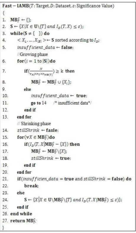
2.5.3 Fast-IAMB ... 21
2.6 MMMB (Max-Min Markov Boundary algorithm)... 23
2.6.1 Bayesian Network and Markov Blanket ... 23
2.6.2 D-separation ... 26
2.6.3 MMPC/MB Algorithm ... 29
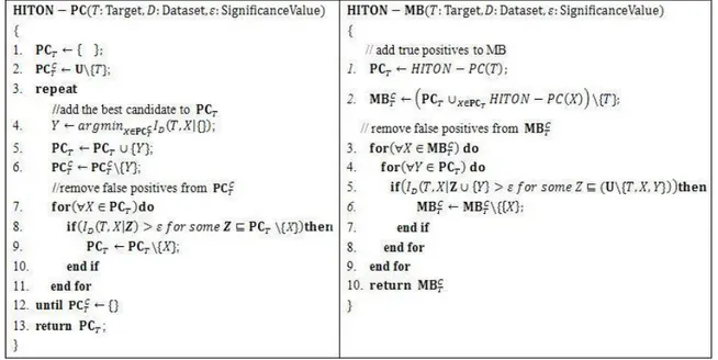
2.7 HITON-PC/MB ... 32
2.8 PCMB ... 34
2.8.1 Motivation and Theoretical Foundation ... 34
2.8.2 Algorithm Specification ... 35
Chapitre 3 A NOVEL ALGORITHM FOR LOCAL LEARNING OF MARKOV BLAKNET : IPC-MB 38 3.1 Motivation ... 38
3.1.1 Data efficiency, accuracy and time efficiency ... 38
3.1.2 Assumptions and overview of our work ... 40
3.2 IPC-MB algorithm specification and proof ... 42
3.2.1 Overall description ... 42
3.2.2 Learn Parent/Child Candidates ... 43
3.2.3 Learn Parents/Children ... 49
3.2.4 Learn Spouses ... 52
3.4 Complexity Analysis ... 56
3.4.1 Time Complexity of FindCanPC ... 56
3.4.2 Time Complexity of IPC-MB ... 61
3.4.3 Memory Requirement of FindCanPC ... 63
3.4.4 Memory Requirement of IPC-MB ... 65
3.4.5 Brief Conclusion on the Complexity of IPC-MB ... 65
3.5 Data Efficiency and Reliability of IPC-MB ... 65
3.6 Analysis of Special Case: Polyrtree ... 67
3.7 Parallel version of IPC-MB ... 69
3.7.1 Overall illustration ... 69
3.7.2 Proof of soundness ... 70
3.7.3 Time and space complexity ... 71
3.7.4 About implementation ... 71
3.8 Conclusion ... 71
Chapitre 4 EMPIRICAL STUDY OF MARKOV BLANKET LEARNING ... 73
4.1 Experiment Design ... 73
4.2 Data Sets ... 73
4.3 Implementation Version of IPC-MB ... 77
4.4 Accuracy ... 78
4.4.1 Small Network: Asia ... 79
4.4.2 Moderate Network: Alarm ... 82
4.4.3 Large Network: Hailfinder and Test152 ... 85
4.4.4 Polytree Network: PolyAlarm (Derived from Alarm) ... 88
4.5 Time Efficiency ... 93
4.5.1 Small Network: Asia ... 94
4.5.2 Moderate Network: Alarm ... 95
4.5.3 Large Network: Hailfinder and Test152 ... 96
4.5.4 Polytree Network: PolyAlarm(Derived) ... 97
4.5.5 Conclusion ... 98
4.6 Data Efficiency ... 101
4.6.1 Relative Accuracy ... 101
4.6.2 Distribution of Conditioning Set Size ... 102
4.7 Summary ... 105
Chapitre 5 TRADEOFF ANALYSIS OF DIFFERENT MARKOV BLANKET LEARNING ALGORITHMS ... 107
5.1 Introduction ... 107
5.2 Category of Algorithms ... 107
5.3 Efficiency Gain by Local Search ... 108
5.4 Data Efficiency ... 108
5.4.1 Data Efficiency is Critical ... 108
5.4.2 Why IAMB is Very Data Inefficient ... 108
5.4.3 PCMB is Data Efficient ... 109
5.4.4 IPC-MB is Data Efficient Too ... 109
5.5 Time Efficiency ... 110
5.5.1 IAMB is Fast but with High Cost ... 110
5.5.2 IPC-MB is Much More Efficient Than PCMB ... 111
5.6 Scalability ... 112
5.8 Approximate Version of IPC-MB ... 114
5.9 Summary ... 116
Chapitre 6 A NOVEL LOCAL LEARNING ALGORITHM OF BAYESIAN NETWORK CLASSIFIER: IPC-MBC ... 118
6.1 Background ... 118
6.2 Structure Learning of Bayesian Network ... 120
6.2.1 Conditional Independence Test Approach ... 120
6.2.2 Score-and-Search Approach ... 121
6.2.3 Statistical Equivalence ... 122
6.3 Motivation, Heuristics and Our Work ... 123
6.4 IPC-MBC Algorithm Specification and Proof ... 124
6.4.1 Overrall Description ... 124
6.4.2 Induce Candidate Parents/Children of Target ... 127
6.4.3 Recognize /Links among / ... 129
6.4.4 Recognize /Links among /Links between and ... 132
6.4.5 Achieve the Skeleton of ... 135
6.4.6 Orientation ... 135
6.4.7 Conclusion ... 136
6.5 Complexity Analysis ... 137
6.6 Empirical Study ... 137
6.6.1 Experiment Design ... 137
6.6.2 IPC-MBC as Markov Blanket Learner ... 139
6.6.3 IPC-MBC as MBC Learner ... 150
6.7 Discussion of Different MBC Learners ... 152
Chapitre 7 CONCLUSION AND PERSPECTIVES ... 155 7.1 Conclusion on Knowledge, Work and Experience Gained ... 155 7.2 Perspectives and Feature Work ... 155 7.2.1 Reduce data passes ... 155 7.2.2 Work with Score-and-Search Structure Learning Algorithms ... 156 7.2.3 Bayesian Network Structure Learning via Parallel Local Learning ... 160 7.2.4 Increasing the Reliability of Induction ... 160 7.2.5 Comparison with Other Feature Selection Algorithms ... 161 BIBLIOGRAPHY ... 162
LIST OF TABLES
Table 3.1: General analysis of the number of CI tests as required in FindCanPC. ... 57 Table 4.1: Feature summary of data sets ... 77 Table 4.2: Accuracy comparison of IAMB, PCMB, IPC-MB and PC over Asia network. ... 79 Table 4.3: Accuracy comparison of IAMB, PCMB, IPC-MB and PC over Alarm network. ... 83 Table 4.4: Accuracy comparison of IAMB, PCMB, IPC-MB and PC over Hailfinder network. 85 Table 4.5: Accuracy comparison of IAMB, PCMB, IPC-MB and PC over Test152 network. ... 85 Table 4.6: Accuracy comparison of IAMB, PCMB, IPC-MB and PC over polytree version
Alarm network. ... 88 Table 4.7: Time complexity comparison of IAMB, PCMB, IPC-MB and PC over Asia network.
... 94 Table 4.8: Time complexity comparison of IAMB, PCMB, IPC-MB and PC over ALARM
network. ... 95 Table 4.9: Time complexity comparison of IAMB, PCMB, IPC-MB over Hailfinder network
( = 0.05). ... 96 Table 4.10: Time complexity comparison of IAMB, PCMB, IPC-MB over Test152 network
( = 0.05). ... 96 Table 4.11: Time complexity comparison of IAMB, PCMB, IPC-MB and PC over PolyAlarm
network. ... 97 Table 4.12: Time complexity comparison of between IAMB/PCMB/IPC-MB and PC. The
comparison is based on the average measures of 20K-Asia experiment, 5K-PolyAlarm experiment, 5K-Alarm, 20K-Hailfinder and 2.5K-Test152 ex-periments respectively. In the table means that x% reduction is achieved compared with PC algorithm; , in contrast, indicates additional x% cost relative to that of PC algorithm. ... 99
Table 4.13: Time complexity comparison of IAMB/PCMB/IPC-MB given example networks with same number of nodes but different density of connectivity. All are
measured in experiments with 5,000 instances. ... 100 Table 5.1: The comparison of IPC-MB to PCMB and IAMB in terms of time efficiency and
accuracy. About time cost, means IPC-MB costs more CI tests than PCMB or IAMB; and about accuracy, means IPC-MB‟s distance to the perfect result is larger than PCMB or IAMB (note: the smaller the distance, the more accurate the result). ... 113 Table 5.2: Trade-off summary over IAMB, PCMB and IPC-MB. ... 116 Table 6.1: Accuracy comparison of PC, IPC-MB and IPC-MBC over Alarm network. ... 139 Table 6.2: Time efficiency comparison of PC, IPC-MB, IPC-MBC (Alarm, = 0.05). ... 141 Table 6.3: Accuracy comparison of PC, IPC-MB+PC and IPC-MBC over Alarm network. ... 143 Table 6.4: Accuracy comparison of PC, IPC-MB+PC and IPC-MBC over PolyAlarm network.
... 144 Table 6.5: Accuracy comparison of PC, IPC-MB+PC and IPC-MBC over Test152 network. .. 146 Table 6.6: Time complexity comparison of PC, IPC-MB+PC and IPC-MBC over Asia
network. ... 147 Table 6.7: Time efficiency comparison of PC, IPC-MB+PC, IPC-MBC (Alarm, = 0.05). ... 148 Table 6.8: Time efficiency comparison of PC, IPC-MB+PC, IPC-MBC (PolyAlarm, = 0.05).
... 149 Table 6.9: Time efficiency comparison of PC, IPC-MB+PC, IPC-MBC (Test152, = 0.05). ... 149 Table 6.10: Accuracy comparison of PC, IPC-MB+PC and IPC-MB over Asia network. ... 150
LIST OF FIGURES
Figure 1-1: An example of a Bayesian network. The parents and children of are the
variables in gray, while additionally includes the textured-filled variable O. The partial network over and are the Markov blanket classifier about as class. ... 5 Figure 2-1: Grow-shrink (GS) algorithm. ... 18 Figure 2-2: IAMB algorithm ... 19 Figure 2-3: Fast-IAMB algorithm. ... 22 Figure 2-4: Three possible patterns about any path through a node in Bayesian network ... 27 Figure 2-5: The Markov blanket of (includes P(arents), C(hildren) and S(pouses)) d-
separates all other nodes given faithfulness assumption. ... 28 Figure 2-6: MMPC/MB algorithm ... 29 Figure 2-7: Two examples that MMPC/MB produces incorrect results ... 30 Figure 2-8: CMMC, Corrected MMPC ... 32 Figure 2-9: HITON-PC/MB algorithm ... 32 Figure 2-10: PCMB Algorithm. ... 36 Figure 3-1: FindCanPC algorithm and its pseudo code. ... 44 Figure 3-2: Possible connections between Non-Descendants/Parents/Children and descendant.48 Figure 3-3: IPC-MB algorithm and its pseudo code. ... 50 Figure 3-4: as output by FindCanPC( ), and the output of typical , i.e. . ... 51 Figure 3-5: An example of network which has the largest size of Markov blanket, and
FindCanPC performs the worst on it. ... 59
Figure 3-6: An example of network which has the largest size of Markov blanket, but
FindCanPC perform the best on it. ... 60
Figure 3-7: A simple example of polytree. The original graph can be found online at
Figure 3-8: Parallel version of IPC-MB. ... 70 Figure 4-1: Asia Bayesian Network including 8 nodes of two states and 8 arcs, along with its
CPTs. For reference purpose, each node is assigned one unique ID, from 0 to 7. The original graph can be found at http://www.norsys.com/netlib/asia.htm. ... 74 Figure 4-2: Alarm Bayesian Network including 37 nodes of two, three or four states (To save
space, the CPTs are ignored). The original graph can be found online at
http://compbio.cs.huji.ac.il/Repository/Datasets/alarm/alarm.htm. ... 75 Figure 4-3: A polytree derived from Alarm Bayesian Network [39]. This graph is created by
BNJ tool. ... 76 Figure 4-4: Distribution of the size of Markov blankets as contained in Asia, Alarm, Poly-
Alarm, Hailfinder and Test152. ... 77 Figure 4-5: The implemented version of FindCanPC that considers reliability of statistical
tests. Its original version can be found in Figure 3-1, and the differences are
illustrated in bold here for comparison convenience. ... 78 Figure 4-6: Comparison of distances given different number of instances (0.1K~20K):
IAMB vs. PCMB vs. IPC-MB vs. PC (Asia, = 0.05, refer to Tableau 4.2 for more information) ... 81 Figure 4-7: Comparison of precision given different number of instances (0.1K~20K):
IAMB vs. PCMB vs. IPC-MB vs. PC (Asia, = 0.05, refer to Tableau 4.2 for more information) ... 82 Figure 4-8: Comparison of recall given different number of instances (0.1K~20K): IAMB
vs. PCMB vs. IPC-MB vs. PC (Asia, = 0.05, refer to Tableau 4.2 for more
information) ... 82 Figure 4-9: Comparison of distances given different number of instances (0.5K~5K): IAMB
vs. PCMB vs. IPC-MB vs. PC (Alarm, = 0.05, refer to Tableau 4.3 for more information) ... 84
Figure 4-10: Comparison of precision given different number of instances (0.5K~5K): IAMB vs. PCMB vs. IPC-MB vs. PC (Alarm, = 0.05, refer to Tableau 4.3 for more information) ... 84 Figure 4-11: Comparison of recall given different number of instances (0.5K~5K): IAMB vs.
PCMB vs. IPC-MB vs. PC (Alarm, = 0.05, refer to Tableau 4.3 for more
information) ... 85 Figure 4-12: Comparison of distances given different number of instances (0.25K~2.5K):
IAMB vs. PCMB vs. IPC-MB vs. PC (Test152, = 0.05, refer to ... 87 Figure 4-13: Comparison of precision given different number of instances (0.25K~2.5K):
IAMB vs. PCMB vs. IPC-MB vs. PC (Test152, = 0.05, refer to ... 88 Figure 4-14: Comparison of recall given different number of instances (0.25K~2.5K): IAMB
vs. PCMB vs. IPC-MB vs. PC (Test152, = 0.05, refer to ... 88 Figure 4-15: Comparison of distances given different number of instances (0.5K~5K): IAMB
vs. PCMB vs. IPC-MB vs. PC (PolyAlarm, = 0.05, refer to Tableau 4.6 for more information) ... 90 Figure 4-16: Comparison of precision given different number of instances (0.5K~5K): IAMB
vs. PCMB vs. IPC-MB vs. PC (PolyAlarm, = 0.05, refer to Tableau 4.6 for more information) ... 90 Figure 4-17: Comparison of recall given different number of instances (0.5K~5K): IAMB vs.
PCMB vs. IPC-MB vs. PC (PolyAlarm, = 0.05, refer to Tableau 4.6 for more information). ... 91 Figure 4-18: Comparison of IPC-MB‟s Precision and Recall (Based on experiments with
Alarm, = 0.05, refer to Tableau 4.3 for more information) ... 93 Figure 4-19: Comparison of increasing rate of CI tests given Alarm and PolyAlarm networks:
IAMB vs. PCMB vs. IPC-MB. ... 101 Figure 4-20: Example distribution of conditioning set size (i.e. the cardinality of conditioning
experiments of Alarm (The upper graph is the average distribution given 500 instances, and the bottom is that measured given 5,000 instances). ... 104 Figure 4-21: Example distribution of conditioning set size (i.e. the cardinality of conditioning
set) as involved in CI tests conducted by IAMB, PCMB, IPC-MB and PC in
experiments of polytree version Alarm (5,000 instances). ... 105 Figure 4-22: Example distribution of conditioning set size (i.e. the cardinality of conditioning
set) as involved in CI tests conducted by IAMB, PCMB, IPC-MB and PC in
experiments of Test152 (2,500 instances). ... 105 Figure 5-1: Output of IAMB (left), PCMB and IPC-MB (right) ... 114 Figure 5-2: The version of FindCanPC that restricts the search space as well as considers
reliability of statistical tests. ... 115 Figure 6-1: Examples of Bayesian classifiers, including Naïve Bayes (upper left),
Tree-Augmented Naïve Bayes (upper right) and Bayesian Network (bottom) ... 119 Figure 6-2: The overall algorithm specification of IPC-MBC ... 126 Figure 6-3: FindCanPC-MBC algorithm specification. ... 127 Figure 6-4: contains all the parents and children of (denoted as since they cannot
be distinguished for now) as connected to , as well as some false positives possibly, i.e. children‟s descendants ( with dotted circle). Note that nodes NOT connected to are not drawn in this graph. ... 129 Figure 6-5: In all connecting to are exactly ‟s parents and children, and they still
cannot be distinguished further. It also contains all the possible links among . Candidate spouses are found to be connected with some . In the graph, all confirmed findings are drawn with solid lines, and non-
confirmed with dotted lines... 132 Figure 6-6: In , spouses are recognized, along with some children of . ... 134 Figure 6-7: In , all the nodes and links of the target MBC are there, with some orientation
Figure 6-8: Distribution of the size of Bayesian network classifier as contained in Asia, Alarm and PolyAlarm, and the size is measured by the number of edges. ... 139 Figure 6-9: Comparison of distances given different number of instances (0.5K~5K): PC,
IPC-MB and IPC-MBC (Alarm, = 0.05, refer to Tableau 6.1 for more
information) ... 140 Figure 6-10: Example distribution of conditioning set size (i.e. the cardinality of conditioning
set) as involved in CI tests conducted by PC, IPC-MB and IPC-MBC in
experiments of Alarm (5,000 instances). ... 142 Figure 6-11: Comparison of the increasing rate of CI tests as required by PC, IPC-MB and
IPC-MBC given more observations (Alarm network, = 0.05). Note: For
displaying and convenient observation purpose, the corresponding number of PC algorithm is divided by 4. ... 142 Figure 6-12: Comparison of distances given different number of instances (0.5K~5K): PC vs.
IPC-MB+PC vs. IPC-MBC (Alarm, = 0.05, refer to Tableau 6.3 for more
information). ... 144 Figure 6-13: Comparison of distances given different number of instances (0.5K~5K): PC vs.
IPC-MB+PC vs. IPC-MBC (PolyAlarm, = 0.05, refer to Tableau 6.4 for the complete data). ... 146 Figure 6-14: Comparison of distances given different number of instances (0.25K~2.5K): PC
vs. IPC-MB+PC vs. IPC-MBC (Test152, = 0.05, refer to Tableau 6.5 for the complete data). ... 147 Figure 6-15: Comparison of distances given different number of instances (0.1K~20K): PC
vs. IPC-MB+PC vs. IPC-MBC (Asia, = 0.05, refer to Tableau 6.10 for more information) ... 152 Figure 6-16: On the output of IPC-MB, the number of CI tests as required by PC to induce
the connectivity is relatively small compared with that of IPC-MB. ... 153 Figure 7-1: The overall procedure: start with a bag of variables, then selected with IPC-MB,
and finally apply further scoring-based search to add the remaining arcs as well as to determine the orientations. v-structure determined by IPC-MB is fixed. ... 157
Figure 7-2: Typical output as returned by IPC-MB. ... 158 Figure 7-3: CI2S-MBC algorithm specification ... 159 Figure 7-4: Adjust the output of IPC-MB to make the scoring work as conventional. ... 159
LIST OF ACRONYMS AND ABBREVIATIONS
Observations
All attributes as contained in
Graph. Here, it is used to refer the directed acyclic graph of one Bayesian network, so , where is the set of nodes, and is the set of directed arcs
Variable or attribute
Variable set or attribute vector, | | Cardinality of set or, size of vector
Target variable, or dependent variable. Significance value, or threshold value
Empty set, or
Variable set excluding
BN The concept of Bayesian network, by default over .
The structure of one Bayesian network, so it is a directed acyclic graph. Parents of in
Children of in Spouses of in
Parents and children of in Descendants of in
, where Non-Descendants of of in
Markov blanket of
Candidate parents and children of Candidate spouses of
Candidate Markov blanket of
Markov blanket classifier of . It is the partial Bayesian network over variables , so it is a directed acyclic graph as well
Bayesian network classifier of , another name of Variable is independent with given
d- is d-separated from by node set
Variable is NOT independent with given
Statistical measure of (in)dependency between and given with data
iff. If and only if, can be represented with or
is connected with in
is connected with in , and the edge is pointing to CI Conditional independence
KS Koller and Sahami‟s algorithm on the induction of GS Grow-Shrink algorithm for the induction of IAMB Incremental Association Markov Blanket
HITON-PC One algorithm proposed to learn Markov blanket /MB
MMPC Max-Min Markov boundary algorithm /MB
PCMB Parents and Children based Markov Blanket algorithm
PC PC algorithm, one classical method for the structure learning of Bayesian network TAN Tree-Augmented Naive Bayes. It can be viewed as a special Bayesian network, so
it is a directed acyclic graph as well. If it refers to a specific model structure, we use as the representation.
Chapitre 1 INTRODUCTION
1.1 Feature selection
Prediction, or classification, on one particular attribute in a set of observations is a common data mining and machine learning task. To analyze and predict the value of this attribute, we need to first ascertain which of the other attributes in the domain affect it. This task is frequently referred to as the feature selection problem. A solution to this problem is often non-trivial, and can be infeasible when the domain is defined over a large number of attributes.
In 1997, when a special issue of the journal of Artificial Intelligence on relevance, including several papers on variable and feature selection, was published, few domains explored used more than 40 features [16, 17]. The situation has changed considerably in the past decade: domains involving more variables but relatively few training examples are becoming common [12, 13, 18]. Therefore, feature selection has been an active research area in the pattern recognition, statistics and data mining communities. The main idea of feature selection is to select a subset of input variables by eliminating features with little or no predictive information, but without sacrificing the performance of the model built on the chosen features. It is also known as variable selection, feature reduction, attribute selection or variable subset selection. By removing most of the irrelevant and redundant features from the data, feature selection brings many potential benefits to us:
Alleviating the effect of the curse of dimensionality to improve prediction performance; Facilitating data visualization and data understanding, e.g. which are the important features
and how they are related with each other;
Reducing the measurement and storage requirements; Speeding up the training and inference process; Enhancing model generalization.
A principled solution to the feature selection is to determine a subset of features that can render of the rest of the features independent of the variable of interest [1, 12, 13]. From a theoretical
perspective, it can be shown that optimal feature selection for supervised learning problems requires an exhaustive search of all possible subsets of features, the complexity of which is known as exponential function of the size of whole features. In practice, the target is demoted to a satisfactory set of features instead of an optimal set due to the lack of efficient algorithms. Feature selection algorithms typically fall into two categories: Feature Ranking and Subset Selection. Feature Ranking ranks all attributes by a metric and eliminates those that do not achieve an adequate score. Selecting the most relevant variables is usually suboptimal for building a predictor, particularly if the variables are redundant. In other words, relevance does not imply optimality [17]. Besides, it has been demonstrated that a variable which is irrelevant to the target by itself can provide a significant performance improvement when taken with others [17, 19].
Subset selection, however, evaluates a subset of features that together have good predictive power, as opposed to ranking variables according to their individual predictive ability. Subset selection essentially divides into wrappers, filters and embedded [19].
In the wrapper approach, the feature selection algorithm conducts a search through the space of possible features and evaluates each subset by utilizing a specific modeling approach of interest as a black box [17], e.g. Naïve Bayes or SVM . For example, a Naïve Bayes model is induced with the given feature subset and assigned training data, and the prediction performance is evaluated using the remaining observations available. By iterating the training and cross-validation over each feature subset, wrappers can be computationally expensive and the outcome is tailored to a particular algorithm [17].
Filter is a paradigm proposed by Kohavi and John [17], and it is similar to wrappers in the search approach. A filter method computes a score for each feature and then select features according to their scores. Therefore, filters work independently of the chosen predictor. However, filters have the similar weakness as Feature Ranking since they imply that irrelevant features (defined as those with relatively low scores) are useless though it is proved not true [17, 19].
Embedded methods perform variable selection in the process of training and are usually specific to given learning algorithms. Compared with wrappers, embedded methods may be more efficient in several respects: they make better use of the available data without having to split the training data into a training and validation set; they reach a solution faster by avoiding retraining
a predictor from scratch for every variable subset to investigate [19]. Embedded methods are found in decision trees such as CART, for example, which have a built-in mechanism to perform variable selection [20].
1.2 Classification benefits from feature selection
In the classic supervised learning task, we are given a training set of labeled fixed-length feature vectors, or instances, from which to induce a classification model. This model, in turn, is used to predict the class label for a set of previously unlabeled instances. While, in a theoretical sense, having more features should give us more discriminating power, the real-world provides us with many reasons why this is not generally the case.
Foremost, many induction methods suffer from the curse of dimensionality. That is, as the number of features in an induction increases, the time requirements for an algorithm grow dramatically, sometimes exponentially. Therefore, when the set of features in the data is sufficiently large, many induction algorithms are simply intractable. This problem is further exacerbated by the fact that many features in a learning task may either be irrelevant or redundant to other features with respect to predicting the class of an instance. In this context, such features serve no purpose except to increase induction time.
Furthermore, many learning algorithms can be viewed as performing (a biased form of) estimation of the probability of the class label given a set of features. In domain with a large number of features, this distribution is very complex and of high dimension. Unfortunately, in the real world, we are often faced with the problem of limited data from which to induce a model. This makes it very difficult to obtain good estimates of the many parameters. In order to avoid over-fitting the model to the particular distribution seen in the training data, many algorithms employ the Occam‟s Razor [13] principle to build as simple a model as possible that still achieves some acceptable level of performance on the training data. This guide often leads us to prefer a small number of relatively predictive features over a large number of features.
If we could reduce the set of features considered by the algorithm, we can therefore serve two purposes. We can considerably decrease the running time of the induction algorithm, and we can increase the accuracy of the resulting model. In light of this, effort has been put on the issue of feature subset selection in machine learning as we mentioned in last section.
1.3 Bayesian Network, Markov blanket and Markov blanket
classifier
Let be the set of features, and as the target variable of interest. is used to refer our problem domain, and it is composed of and , i.e. . A Markov blanket of is any subset of that renders statistically independent from all the remaining attributes (see Definition 7.4). Koller and Sahami [1] first showed that the Markov blanket of a given target is the theoretically optimal set of attributes to predict its class value. If the probability distribution of can be faithfully (see Definition 1.3) represented by a Bayesian network (BN, see Definition 1.1) over , then the Markov blanket of is unique, just equal to its Markov boundary(see
Definition 7.4), and it consists of the union of the parents, children and spouses of in the
corresponding BN [2]. Besides, the partial Bayesian network over the Markov blanket of plus itself is called Markov blanket classifier, or Bayesian network classifier (see Definition 1.5). Figure 1-1 illustrates a Bayesian network, Markov blanket of and Markov blanket classifier with as the target (or class).
Definition 1.1 (Bayesian Network) A Bayesian network consists of a directed acyclic graph
(DAG) an a set of local distributions. is composed of nodes and edges , i.e. .
Definition 1.2 (Conditional Independence) Two sets of variables, and , are said to be
conditionally independent given some set of variables if, for any assignment of values , and to the variables , and respectively, . That is, gives us no information about beyond what is already in . We use in the remaining text to denote this conditional independence relationship.
Definition 1.3 (Faithfulness Condition) A Bayesian Network and a joint distribution are
faithful to one another iff. every conditional independence entailed by the graph and the Markov Condition is also present in [2].
Definition 7.4 (Markov blanket) A Markov blanket of an attribute is any subset of
for which is conditionally independent with given the values of . A set is called a Markov boundary of if none of its proper subsets satisfy this condition.
Definition 1.5 (Markov blanket classifier) Given a Bayesian network over the target variable
and attributes , the partial DAG over is called the Markov Blanket Classifier, or Bayesian Network Classifier about , and denoted as or .
Definition 1.6 (Markov Condition) Given the value of parents, is conditionally independent
with all its non-descendants, denoted as , excluding its parents , i.e. .
Theorem 1.1 If a Bayesian network and a joint distribution are faithful to one another, then
for every attribute , the Markov blanket of is unique and is the set of parents, children and spouses of .
Figure 1-1: An example of a Bayesian network. The parents and children of are the variables in gray, while additionally includes the textured-filled variable O. The partial network over and are the Markov blanket classifier about as class.
Let , and denote the parents, children and spouses of respectively, the Markov
blanket of , denoted as , then is the union of , and (see Theorem 1.1), i.e. for short. Given this knowledge, of any is easily to be obtained if the Bayesian network over is known. However, having to learn the Bayesian Network in order to learn can be painfully time consuming [21]. Hence, how to learn but without having to learn the BN first became the goal of many who are interested to apply Markov blanket as feature selection.
Bayesian network, Markov blanket and Markov blanket classifier concepts are closely related given the faithfulness assumption. They will be frequently mentioned in the remaining text since our goals are efficient learning of Markov blanket and Markov blanket classifier. Chapitre 2 to
Chapitre 5 are about the learning of Markov blanket given a target of interest. The Markov blanket is important because
It is the optimal feature subset for the prediction of , and feature selection is an important data preprocessing step for most machine learning and data mining tasks;
It is closely related to the Markov blanket classifier since the later is just a DAG over and . Understanding this concept well will be helpful to understand our work on Markov blanket classifier;
Given the Markov blanket of , all existing structure learning algorithms of Bayesian network are applicable to induce the Markov blanket classifier. Since the feature space is greatly reduced, the remaining structure learning is expected to be much more efficient than using all features directly;
Our algorithm for inducing the Markov blanket classifier of is an extension of our algorithm on the induction of Markov blanket.
We return to the concept of Markov blanket classifier Chapitre 6.
1.4 KS and related algorithms
Following Koller and Sahami‟s work (KS), many others also realized that the principled solution to the feature selection problem is to determine a subset of features that can render the rest of all other features independent of the variable of interest [12, 13, 18, 21, 22]. Based on the findings that the full knowledge of is enough to determine the probability distribution of and that the values of all other variables become superfluous, we normally can have a much smaller group of variables in the final classifier, reducing the complexity of learning and resulting with a simpler model, but without sacrificing classification performance [2, 3, 4].
Although Koller and Sahami theoretically proved that Markov blanket is the optimal feature subset for predicting the target, the algorithm as proposed by them for inducing is approximate, guaranteeing no correct outcome. There are several attempts to make the induction more effective and efficient, including GS (Grow-Shrink) [23, 24], IAMB (Iterative Associative Markov Blanket) and its variants [12, 18, 22], MMPC/MB (Max-Min Parents and
Children/Markov Blanket) [21], HITON-PC/MB[25], PCMB(Parent-Child Markov Blanket learning) [13] and our own work [10, 11, 26, 27], IPC-MB (Iterative Parents-Children based search of Markov Blanket), which will be discussed later. To our best knowledge, this list contains all the published primary algorithms. In next chapter, we will review these MB local learning algorithms in terms of theoretical and practical considerations, based on our experience gained from both academic research and industry implementation.
1.5 Motivation, contributions and overall structure
This project was initiated during my time in SPSS® (http://www.spss.com, acquired by IBM in 2009), where they needed a component of Bayesian Network for classification on widely deployed Clementine® (http://www.spss.com/software/modeling/modeler/, now named as PASW Modeler®). The greatest merit of a Bayesian Network is that its graphical model allows us to observe the relations of the variables involved, which is very important for diagnosis application. However, this component is designed primarily for classification, i.e. predicting the state of some target variable given input features, instead of general modeling. Regarding this goal, Pearl and Koller‟s works tell us that only the Markov blanket is effective in the prediction, which means that the partial Bayesian Network over the target and its Markov blanket is enough. This partial Bayesian Network is called Markov Blanket Classifier (MBC) or Bayesian Network Classifier (BNC) by us, to distinguish it from the whole Bayesian Network. It has all the merits of a general Bayesian Network, but it is “customized” for classification. In a naïve way, we can induce the Bayesian Network over all input variables first, and then extracting the MBC becomes trivial. This is possible and it requires no extra research effort, all existing conventional algorithms for the structure learning of Bayesian Network are there for reference. However, the learning of Bayesian network is known as an NP-complete problem, and the complexity grows exponentially in term of the number of inputs and the number of states of each individual input [3]. Therefore, the goal is to induce the MBC directly without having to learn the Bayesian Network first.
Koller and Sahami opened a new window, and many more fruitful studies have been done, along with many published outcomes. Given a bag of features , these algorithms allow the induction of without requiring to know the Bayesian Network over in advance. With , the problem space generally is greatly reduced in dimension; besides, all existing algorithms for the structure learning of Bayesian Network are applicable, and they are expected to yield the


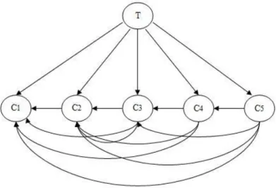


![Figure 4-3: A polytree derived from Alarm Bayesian Network [40]. This graph is created by BNJ tool](https://thumb-eu.123doks.com/thumbv2/123doknet/2330638.31615/108.918.113.760.101.379/figure-polytree-derived-alarm-bayesian-network-graph-created.webp)