HAL Id: tel-01379206
https://hal-lirmm.ccsd.cnrs.fr/tel-01379206
Submitted on 11 Oct 2016HAL is a multi-disciplinary open access archive for the deposit and dissemination of sci-entific research documents, whether they are pub-lished or not. The documents may come from teaching and research institutions in France or abroad, or from public or private research centers.
L’archive ouverte pluridisciplinaire HAL, est destinée au dépôt et à la diffusion de documents scientifiques de niveau recherche, publiés ou non, émanant des établissements d’enseignement et de recherche français ou étrangers, des laboratoires publics ou privés.
Sciences et Techniques du Languedoc
P
H
.D T
HESIS
présentée au Laboratoire d’Informatique de Robotique et de Microélectronique de Montpellier pour
obtenir le diplôme de doctorat
Spécialité : Informatique
Formation Doctorale : Informatique
École Doctorale : Information, Structures, Systèmes
Mining Object Movement Patterns from Trajectory Data
par
PHAN N
HAT
H
AI
Version du September 30, 2013 Supervisor
Mme. Maguelonne TEISSEIRE, Research Director . . . IRSTEA, Montpellier Joint supervisor
M. Pascal PONCELET, Professor . . . LIRMM, Université Montpellier II Reviewers
M. Osmar ZAÏANE, Professor . . . University of Alberta M. Arno SIEBES, Professor . . . Utrech University Examinators
M. Francesco BONCHI, Senior Researcher. . . .Yahoo! Research Lab M. Bruno CREMILLEUX, Professor . . . Université de Caen M. Dino IENCO, Researcher . . . IRSTEA, Montpellier
First and foremost I want to thank my advisors: Dr. Dino Ienco, Prof. Pascal
Poncelet and Dr. Maguelonne Teisseire. It has been an honor to be their PhD
student. I appreciate all their valuable support of time, ideas, and funding
to make my PhD experience productive and stimulating. The joy and
enthusiasm they have for their research was contagious and motivational
for me, even during tough times in the PhD pursuit. The members of the
Tatoo team have contributed immensely to my personal and professional
time at Irstea, Lirmm, and University of Montpellier 2. The team has been a
source of friendships as well as good advice and collaboration. I am
especially grateful for the fun team members who stuck it out with me
during my PhD duration: Hugo Alatrista-Salas, Mickaël Fabrègue, and
Flavien Bouillot. We worked together on the mining trajectories on Tweets
experiments, and I very much appreciated his enthusiasm, intensity,
willingness to do all the tasks. In additionally, I am also thankful to Amal
Zine El Aabidine for her help in mining trajectories from gene data source. I
thank Prof. Donato Malerba (University of Bari) for not only proposing the
multi-relational gradual pattern idea but also advising me on the very
interesting work. Under his support, we are able to extract an novel kind of
gradual patterns based on two different point of views. In my later work of
Communication Graph Compression, I am grateful to Dr. Francesco Bonchi
(Senior Researcher at Yahoo! Lab) for his support, guidance and all fun
along during three months of my internship at Yahoo! Research Lab,
Barcelona. I gratefully acknowledge the funding sources that made my PhD
work possible. I was funded by the French National Centre for Scientific
Research (CNRS). My work was also supported by the LIRMM - IRSTEA
Laboratories. For this dissertation I would like to thank my reading
committee members: Prof. Osmar Zaiane, Prof. Arno Seibes, Dr. Francesco
Bonchi, and Prof. Bruno Cremilleux for their time, interest, helpful
with a love of science and supported me in all my pursuits. And most of all
for my loving, supportive, encouraging, and patient girl friend Huong whose
faithful support during the final stages of this PhD is so appreciated. Thank
you. PHAN Nhat Hai, Irstea-Lirmm Labs, University Montpellier 2, October
2013.
Contents iii
List of Figures 1
List of Tables 4
1 Introduction 7
1.1 Illustrative Example and Motivations . . . 8
1.2 Contributions . . . 9
2 Related Work 15 2.1 Preliminary Definitions . . . 15
2.2 Object Movement Pattern Mining . . . 19
3 All in One: Mining Multiple Movement Patterns 23 3.1 Object Movement Patterns in Itemset Context . . . 23
3.2 Frequent Closed Itemset-based Object Movement Pattern Mining Algorithm 29 3.2.1 GeT_Move . . . 29
3.2.2 Incremental GeT_Move . . . 31
3.3 Preliminarily Experimental Results . . . 34
3.3.1 Effectiveness. . . 35
3.3.2 Efficiency. . . 37
3.3.3 Toward A Parameter Free Incremental GeT_Move Algorithm . . . 40
3.3.4 Object Movement Pattern Mining Algorithm Based on Explicit Com-bination of FCI Pairs . . . 45
4.3 Discovering of Fuzzy Closed Swarms . . . 59
4.4 Experimental Results . . . 62
4.4.1 Effectiveness. . . 63
4.4.2 Parameter Sensitiveness . . . 64
4.5 Discussion . . . 67
5 Mining Time Relaxed Gradual Moving Object Clusters 69 5.1 Introduction . . . 70
5.2 Problem Statement . . . 72
5.3 Discovering Maximal Time Relaxed Gradual Trajectory Patterns . . . 74
5.3.1 ClusterGrowth Approach . . . 76
5.3.2 The ClusterGrowth Implementation. . . 78
5.4 Preliminarily Experimental Results . . . 80
5.4.1 Effectiveness and Pattern Meaning . . . 81
5.4.2 Parameter Sensitiveness . . . 83
5.5 Mining Representative Gradual Trajectory Patterns . . . 85
5.5.1 Problem Statement . . . 87
5.5.2 Encoding Scheme. . . 88
5.5.3 Complexity Analysis . . . 90
5.5.4 Mining top-K Representative rGpatterns . . . 90
5.6 Experimental Results on Mining Representative rGpatterns . . . 96
5.7 Discussion . . . 100
6 Mining Representative Movement Patterns through Compression 101 6.1 Introduction . . . 101
6.2 Problem Statement . . . 103
6.3 Encoding Scheme . . . 104
6.3.1 Movement Pattern Dictionary-based Encoding . . . 104
6.3.2 Overlapping Movement Pattern Encoding . . . 105
6.4 Mining Compression Object Movement Patterns . . . 108
6.4.1 Naive Greedy Approach . . . 108
6.5 Experimental Results . . . 110
6.6 Discussion . . . 113
7 Mining Multi-Relational Gradual Patterns 115 7.1 Introduction . . . 115
7.2 Preliminarily Definitions . . . 117
7.2.1 Multi-Relational Data . . . 117
7.2.2 Gradual Pattern: Single Relation vs Multi-Relations . . . 117
7.2.3 Multi-Relational Gradual Pattern. . . 118
7.3 Pattern Occurrences . . . 120
7.4 Pattern Support . . . 121
7.4.1 Kendall’s⌧-based Multi-Relational Gradual Pattern Support . . . 123
7.4.2 Gradual Support . . . 127
7.5 Multi-Relational Gradual Pattern Mining Algorithms . . . 130
7.5.1 Mining Mono-Relational Gradual Patterns . . . 130
7.5.2 Discovering Multi-Relational Gradual Patterns . . . 132
7.6 Experimental Results . . . 135
7.6.1 Multi-Relational Gradual Patterns . . . 136
7.6.2 Efficiency and Pattern Distribution . . . 136
7.7 Related Work . . . 138
7.8 Discussion . . . 139
8 Applications 143 8.1 Introduction . . . 144
8.2 The MULTI_MOVESystem Architecture . . . 144
8.3 Other Applications. . . 146
8.3.1 Mining Trajectories on Genes. . . 146
8.3.2 Mining Trajectories on Tweets . . . 148
8.4 Discussion . . . 151
9 Conclusion & Perspectives 153 9.1 Conclusion . . . 153
9.2 Streaming GeT_Move: Mining Representative Movement Patterns from Streaming Trajectory Data . . . 154
9.3 CorGpattern: Combined Time Relaxed Gpattern . . . 155
9.3.1 CorGpattern Definition . . . 156
9.3.2 CoClusterGrowth: Discovering Maximal CorGpatterns . . . 157
9.4 Directly Mining Representative Movement Patterns through Compression . 157 9.5 Completed Mining Multi-Relational Gradual Patterns . . . 158
9.6 Trajectory Mining on Diverse Applications . . . 159
1.1 A running example of moving object data. . . 8
1.2 Our three step framework on mining and managing object movement patterns. 10 2.1 An example of swarm and convoy extracted from the Figure 1.1. . . 16
2.2 A group pattern example. . . 18
2.3 A periodic pattern example. . . 19
3.1 A swarm from our running example in Figure 1.1. . . 25
3.2 A convoy from our running example in Figure 1.1. . . 26
3.3 The main process. . . 30
3.4 A case study example. (b)-ci1 (resp. ci2, ci3) is a frequent closed itemset ex-tracted from block 1 (resp. block 2). . . 31
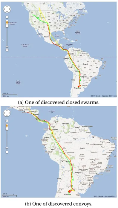
3.5 An example of patterns discovered from Swainsoni dataset. . . 36
3.6 Running time on Swainsoni dataset. . . 38
3.7 Running time on Buffalo dataset. . . 39
3.8 Running time on Synthetic dataset. . . 40
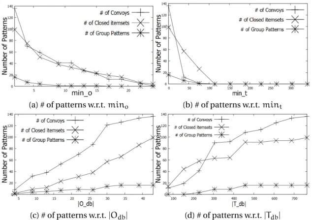
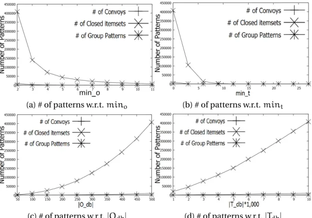
3.9 Number of patterns on Swainsoni dataset. Note that # of frequent closed item-sets is equal to # of closed swarms. . . 41
3.10 Number of patterns on Buffalo dataset. Note that # of frequent closed itemsets is equal to # of closed swarms. . . 42
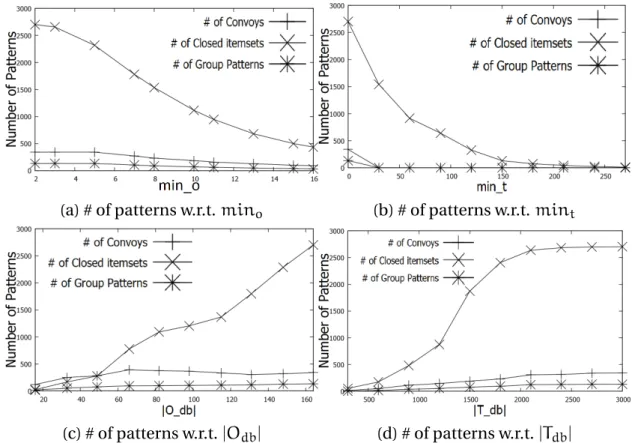
3.11 Number of patterns on Synthetic dataset. Note that # of frequent closed item-sets is equal to # of closed swarms. . . 43
3.12 Running time w.r.tminoon large Synthetic dataset. . . 43
3.13 Running time w.r.t block size. . . 44
4.1 An example of moving object clusters. o3, o4are moving objects,c1, . . . , c5, c10
are clusters which are generated by applying some clustering techniques and A,
C, D, E, H are spatial regions. . . . 56
4.2 Membership degree functions for fuzzy time gaps. . . 57
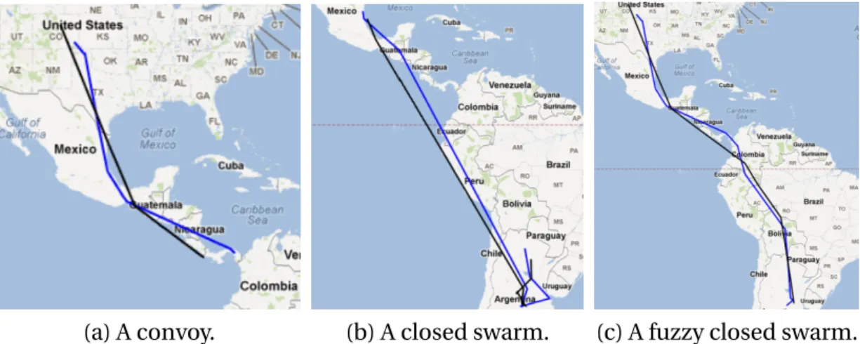
4.3 A fuzzy closed swarm example from our running example in Figure 1.1. . . 58
4.4 An example of extracted patterns from Swainsoni dataset. The two object names are ’SW22’ and ’SW40’. . . 64
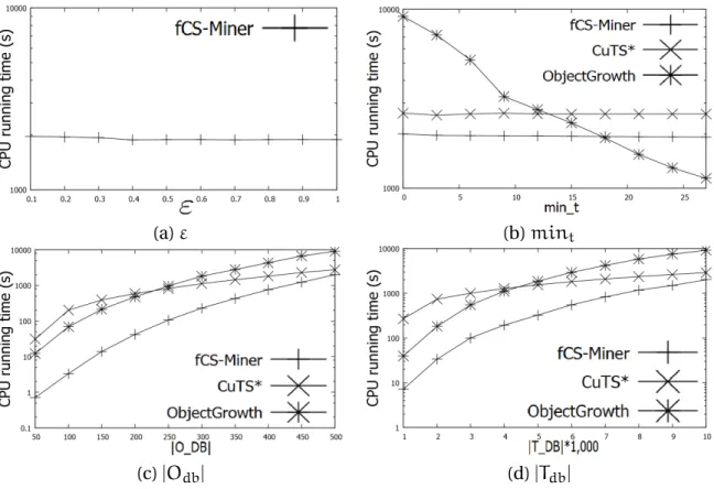
4.5 Running time on Synthetic Dataset. . . 65
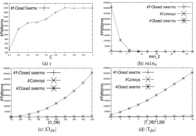
4.6 Number of patterns on Synthetic Dataset. . . 66
4.7 Influence ofTGi(X)on #patterns through".. . . 66
5.1 An example of gradual moving object clusters from running example in Figure 1.1. . . 70
5.2 An example of time relaxed gradual trajectory pattern. . . 71
5.3 An example of uninteresting rGpattern and sliding window (w= 2). . . 73
5.4 An object bit set configuration example. . . 75
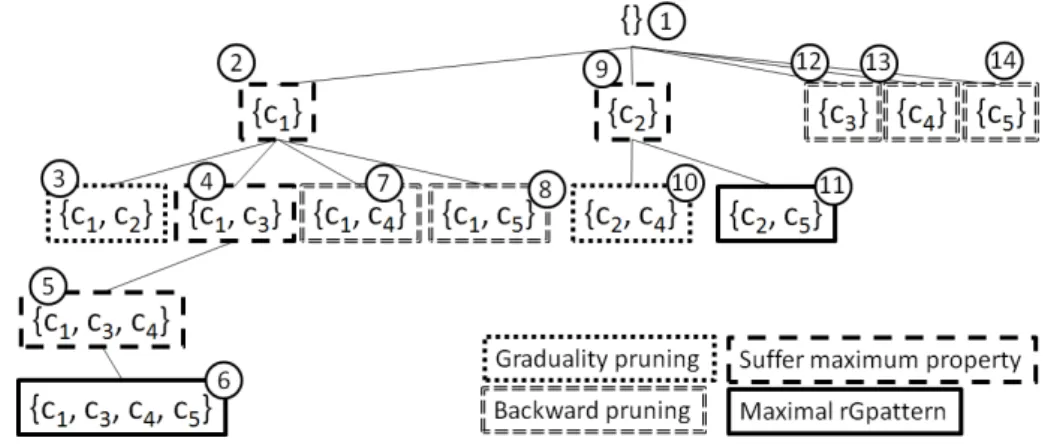
5.5 ClusterGrowth search space of the running example in Figure 5.1 with §=’∏’, mint= 1andw= 3. . . 76
5.6 An example of extracted patterns from Swainsoni dataset (best viewed in color). 82 5.7 Running time on Buffalo Dataset. . . 83
5.8 Running time on Synthetic Dataset. . . 84
5.9 Number of patterns on Buffalo Dataset. For conciseness sake, #Interesting Max-imal rGpatterns is denoted as #rGpatterns. . . 85
5.10 Number of patterns on Synthetic Dataset. For conciseness sake, #Interesting Maximal rGpatterns is denoted as #rGpatterns. . . 86
5.11 An example of two types of rGpatterns. cand o respectively are cluster and object,(oi, cj) = 1meansoibelongs to clustercj. Blurred rectangle is the over-lapping part between two rGpatterns. . . 88
5.12 COMPOGPalgorithm in action.. . . 91
5.13 An example of directly evaluating compression gain ofC∏.Cusedo i andO used cj are lists of blurred rectangles. . . 93
5.14 An illustration of DICOMPOGP in Table 5.4. c5 is the largest cluster among
c1, . . . , c8. . . 94
5.15 Compressibility (higher is better) of different algorithms. . . 97
5.16 Running time of different algorithms.. . . 98
5.17 rGpattern generation task vs post-processing task vs DICOMPOGPon Synthetic dataset. . . 99
5.18 The DiCompoGp scalability on Synthetic dataset. . . 99
6.1 An example of moving object database. Shapes are movement patterns,oi, ci respectively are objects and clusters. . . 102
6.2 An example of pattern overlapping, between closed swarms (rectangles) and rGpatterns (step shapes), in Figure 1.1. Overlapping clusters arec1, c3, c4, c5and c6.. . . 102
6.3 An example of the approach. . . 105
6.4 Top-3 typical compression patterns. . . 111
6.5 Compressibility (higher is better) of different algorithms. . . 112
6.6 Running time.. . . 113
7.1 A Financial database (from PKDD CUP 99). . . 120
7.2 A 1:N relation example (best view in color). . . 122
7.3 Loan./ Account. . . 122
7.4 A M:N relation example. (t30, t50) does not support the pattern p = {Book.price>, Client.birthday<}since(C2, C3)62occ(Client.birthday<) . . 125
7.5 An illustrative example of Binary matrix of orders in Table 7.1. . . 131
7.6 Graph of the Financial MRD in Figure 7.1. . . 133
7.7 mrGpsearch space of the graph in Figure 7.6. . . 135
7.8 (a)(b)-Running time and #patterns on the Financial database. (c)(d)-Running time and #patterns on the Thrombosis database. . . 137
7.9 Number of redundant patterns in Financial database. . . 138
7.10 Multi-relational gradual pattern distribution with min∏0.15.. . . 139
8.1 The MULTI_MOVESystem Architecture. . . 145
8.2 The Graphical Visualization Interface. . . 145
8.3 The graphical visualization interface of gene expression tool.. . . 149
8.4 Another graphical visualization interface of gene expression tool. . . 150
8.5 An example of a trajectory that can be extracted from tweets.. . . 150
9.1 An example of Streaming GeT_Move. . . 155
9.2 An example of CorGpattern extracted from our running example, i.e. Figure 1.1. 156 9.3 DiCompo algorithm in action. . . 158
9.4 Left: Subset of a Quickbird satellite image of Rostock (© DigitalGlobe, Inc., 2011), right: derived land cover classes.. . . 160
2.1 An example of a moving object database. . . 16
2.2 Overview of movement pattern methods and applications. . . 21
3.1 Cluster matrix from our running example in Figure 1.1. . . 24
3.2 Periodic cluster matrix in Figure 2.3. . . 27
3.3 Closed Itemset Matrix.. . . 33
3.4 An example of FCI binary presentation. . . 45
3.5 Fully nested blocks on datasets. . . 49
4.1 Cluster matrix corresponding to our example in Figure 1.1. . . 60
5.1 Notation Description. . . 74
5.2 An example of a reconfigured spatio-temporal database in Figure 5.1. . . 75
5.3 An illustrative example of data and dictionary in Figure 5.11. ¯1and ¯2 respec-tively are pattern types:C∏andC∑. . . 89
5.4 An illustrative example of moving object data.. . . 94
5.5 The number of all the rGpatterns in datasets. . . 98
6.1 An illustrative example of database and dictionary in Figure 6.2. ¯0, ¯1and ¯2 re-spectively are pattern types: closed swarm,rGpattern∏andrGpattern∑. . . . 104
6.2 Correlations between pattern pand patternp0 in F. O, andX respectively mean "overlapping allowed, regular encoding", "overlapping allowed, no encod-ing" and "overlapping not allowed". . . . 106
7.1 Gradual support vs Kendall’s⌧support. . . 127
7.2 Interesting Patterns. . . 142 8.1 Example of matrix query to compare extracted trajectories for HIV-2, R5, and X4. 148 8.2 Cluster matrix corresponding to gene dataset.. . . 148
1
Introduction
With the rapid development of positioning technologies, sensor networks, and online social media, spatio-temporal data is now widely collected from smartphones carried by people, sensor tags attached to animals, GPS tracking systems on cars and airplanes, RFID tags on merchandise, and location-based services offered by social media. Indeed, analyz-ing spatio-temporal data generated from these systems frames many research problems and high-impact applications:
. Understanding animal movement is important to addressing environmental chal-lenges such as climate and land use change, bio-diversity loss, invasive species, and infectious diseases.
. Traffic patterns help people understand conditions of road networks and better design future transportation systems; analyzing driving patterns combining with weather conditions could improve routing systems.
. Unusual vessel trajectory could be a sign of smuggling; outlying taking-off/landing patterns could be a dangerous signal for aviation; and detection of suspicious human movements could help prevent crimes and terrorism.
Motivated by the huge benefit of many applications, a lot of researchers have been fo-cusing their research motivation to spatio-temporal data mining. One of the key tech-niques is to analyze such datasets for meaningful patterns, called moving object clusters [7] [17] [18] [23]. A moving object cluster can be defined in both spatial and temporal dimensions: (1) a group of moving objects should be geometrically close to each other, (2) they should be together for at least mint timestamps. In this context, many recent
studies have been conducted to mine moving object clusters including flocks [7] [30] [39], moving clusters [19] [17], convoy queries [18] [2], k-star [29], closed swarms [23] [9], trav-eling companions [28], group patterns [32], periodic patterns [24], etc. To extract these kinds of patterns, many algorithms have been proposed such asCuTS§(convoy mining),
Figure 1.1: A running example of moving object data.
ObjectGrowth(closed swarm mining),VG-Growth(group pattern mining),BFE(flock mining), Periodica(periodic pattern mining), etc. Interested readers may refer to [14] where descriptions of the most efficient approaches and patterns are presented.
For instance, let us consider a database in which there are four cars moving during the time and their locations are reported by GPS system. We have 4 cars moving from t1 to t999, 8i2[1 : 10],ci is a cluster generated by applying clustering technique as presented
in Figure 1.1. In most of the chapters, we will use (a part of) this running example for enhancing some particularities that are addressed in the chapter. One of the extracted convoys can be "the two cars,o3ando4, are consecutively moving together fromt1tot4"
or a potential closed swarm is "the two cars, o1 and o2, are moving together from t2 to t999, from B to L", etc. Even though these kinds of patterns are meaningful, there are some
challenging issues that limit their utility.
1.1 Illustrative Example and Motivations
In this section, we will give an example to generally present challenging issues and our motivations in object movement pattern mining.
1) The first issue is how to efficiently manage different kinds of patterns? Indeed, given a specific dataset, e.g. see Figure1.1, it is difficult to know which kind of patterns is useful to analyze the data. Intuitively, that could be a set of closed swarms indicate that the cars
o1ando2or the carso3ando4are moving together. However, that also could be a set of
moving object clusters state that the carso1, o2, o3ando4are moving together fromCto DtoEtoF, etc.
To deal with this issue, one of potential solutions is employing all the existing ap-proaches, each of which extracts a specific pattern, to obtain all kinds of patterns. Then, user can analyze the final results to understand the object movement behavior. Naturally, the computation is costly and time consuming since we need to execute different algo-rithms consecutively. Additionally, in some applications object locations are continuously
updated, e.g. cars report their locations by using Global Positioning System (GPS). There-fore, new data is always available and it means that we need to execute again and again the algorithms on the entire data to update the final results. This is of course, cost-prohibitive and time consuming as well.
2) The second issue is that the existing patterns are relevant and help us to fully under-stand the complex and unpredictable behavior of moving objects or not. For instance, they require the group of moving objects to be together for at leastminttimestamps, i.e. could
be consecutive or completely be non-consecutive, which might not be practical in the real cases. Enforcing consecutive time constraint may results in loosing meaningful patterns while completely relax this constrain may generate large amount of extraneous patterns.
For instance, see Figure1.1, enforcing the consecutive time constraint results in losing of the pattern "the two cars,o1ando2, are moving together fromBtoEand toF" since they
are not close each other at timet3. While completely relax this constraint will generate the extraneous patterns such as "the two cars,o1ando2, are moving together fromBtoEtoF
toGtoKand toL". This pattern are irrelevant because they meet each other atLafter 949 timestamps by chance and not actually moving together fromKtoL.
Another illustrative example is that the traditional movement patterns usually focus on an unchanged group of objects and thus they cannot capture the object moving trend. Indeed, objects can step by step getting together to go to some place or leaving each other from that place.
For instance, in Figure1.1, "all the cars are gathering atEafterAtoCand toD". This phenomenon is involved in many real world applications such as traffic congestion, animal or population migration, location prediction, etc. Therefore, it demands the definition of novel movement pattern models to enrich the application benefit.
3) Naturally, end user can be overwhelmed by a huge number of extracted patterns al-though only a few of them are useful. Indeed, thousand of patterns representing redundant knowledge clearly poses limit in their usefulness. However, relatively few researchers have addressed the problem of reducing movement pattern redundancy.
4) The potential utility of the developed spatio-temporal mining tools must be justi-fied in their applicable field. One of our ultimate goals is to develop techniques that not only benefit the computer science society, but more importantly, are applicable to vari-ous interdisciplinary science and engineering fields. Therefore, it is always crucial for us to emphasize the practicability of our methods. Performance measures of the developed tools in terms of accessibility, scalability, reliability and other human factors also need to be carefully studied, in order to provide answers to concerns from domain experts.
1.2 Contributions
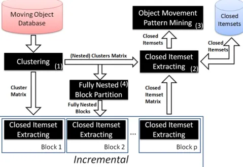
All of the mentioned issues have been addressed in my thesis. We propose a three step framework, i.e. Figure1.2. First of all, we develop a unifying approach to extract and
man-Figure 1.2: Our three step framework on mining and managing object movement patterns.
age multiple patterns. Second, we discover novel kinds of movement patterns and efficient algorithms to mine them. To select informative patterns from thousand of very redundant ones, we further design a compression step based on Minimum Description Length prin-cipal. To justify the utility of the proposed concepts and developed approaches, we also supply a demonstration system, named MULTI_MOVE, which is designed to efficiently and
automatically extract different movement patterns. Our contributions are generally pre-sented as follows:
All in One: Mining Multiple Movement Patterns. Designing a unifying approach which can manage multiple movement patterns is very challenging. This is because: 1) there are many kinds of patterns and each of which have their own characteristics. 2) Additionally the results need to be reusable to obtain the final results when new data is available. 3) Obtaining the optimal parameters is a difficult task for most of algorithms which require parameter setting.
All these challenging issues have been throughly considered and well addressed in my proposed method, GET_MOVE[12]. The basic idea of GET_MOVEis to reconfigure moving object data to a cluster matrix then movement patterns will be redefined in an itemset context. Next, frequent closed itemset will be adopted to efficiently extract closed itemsets from which movement patterns can be mined.
Fuzzy Moving Object Clusters. To soften the consecutive time constraint, the key chal-lenge is to deal with the time gap between a pair of clusters since: 1) it is difficult to rec-ognize which size of a time gap is relevant or not, 2) we need to know when the patterns should be ended to eliminate uninteresting ones.
gap participation index. Obtained patterns are of the type "the two cars,o1 and o2, are
moving together from B to E to E to G and to K with 60% weak, 20% medium and 20% strong time gaps", see Figure1.1. These patterns are characterized by their time gap frequency (or support), which is by definition the proportion of time gaps involved in the patterns. To extract all the fuzzy closed swarms, we propose a novel itemset-based property so that GET_MOVEcan be employed to gather all the fuzzy closed swarms.
Time Relaxed Gradual Trajectory Patterns. A gradual moving object cluster is a list of moving object clusters which satisfy the graduality constraint and integrity condition during at leastminttimestamps. The graduality constraint can be the increase or decrease
of the number of objects and the integrity condition can be that all the objects should remain in the next cluster.
As exemplified in Figure1.1, the retrieved knowledge from traditional patterns can be "the two cars,o1ando2, are moving together fromt2tot6" or "the two cars,o3ando4, are moving together fromt1tot4". Even if these patterns are relevant, they do not really present
the actual moving behavior which can be "fromt1tot4, as time passes, the more cars are
following the trajectory {A i C i D i E}".
To avoid finding redundant rGpatterns, we only focus on discovering the complete set of maximal rGpatterns. The basic idea is that ifCis a rGpattern, it is unnecessary to output any subsetC0ofCeven ifC0may also satisfy rGpattern requirements.
Efficiently extracting of complete set of maximal rGpatterns in a large moving object data, denoteddb, is a non-trivial task. First, the size of all possible combinations is expo-nential, i.e. approximately2|Cdb|whereC
dbis the set of all clusters extracted from the data dband|Cdb|is significantly large. Second, none of previous work (i.e. frequent pattern mining [1] [15], moving object clusters [7] [17] [18] [23]) solves exactly the same issue as finding maximal rGpatterns. This is because they do not address the graduality in terms of itemsets or moving clusters. However, graduality is a key feature in rGpattern context. Thus, the discovery of rGpatterns introduces a new problem that needs to be solved by specifically designed techniques.
Facing the huge potential search space, we propose an efficient approach, named CLUSTERGROWTH, which shares the same spirit with the ObjectGrowth algorithm [23] but
different in terms of design and goal. In CLUSTERGROWTH, we design two efficient rules which are Graduality Pruning and Backward Pruning to end unnecessary further search. After cutting a great portion of invalid candidates through the pruning rules, we perform a further check, i.e. Actual Maximum Checking, to report interesting maximal rGpatterns on-the-fly. This final step avoids using more space to store candidates and extra time for post-processing.
To enrich the utility of the rGpattern concept, we adapt the Minimum Description Length (MDL) principle for mining representative rGpatterns. An encoding scheme which is designed to deal with different kinds of overlapping rGpattern structures is proposed. We show that mining representative rGpatterns is NP-Hard and therefore we propose two heuristic algorithms to extract compressing rGpatterns. The first algorithm, named COM
-This means that using only a single type of patterns is not sufficient to supply an insightful picture of the whole database.
Motivating by these issues, we develop a Minimum Description Length (MDL)-based approach that is able to compress spatio-temporal data combining different kinds of mov-ing object patterns. The core of the method is to design and encodmov-ing scheme for different movement patterns, and then an approach which allow overlapping between them. The proposed method results in a rank of the patterns involved in the summarization of the dataset.
MULTI_MOVE System. Despite the growing demands for diverse applications, there
have been few scalable tools for mining massive and sophisticated moving object data. Even if some tools are available for extracting patterns (e.g. [33]), they mainly focus on specific kinds of patterns at a time. Obviously, when considering a dataset, it is quite dif-ficult for the decision maker to know in advance which kinds of patterns are embedded in the data. To cope with this issue, we propose the MULTI_MOVE system to reveal,
au-tomatically and in a very efficient way, collective movement patterns like convoys, group patterns, closed swarms, moving clusters and also periodic patterns. Starting from the results of MULTI_MOVE, the user can then visualize, browse and compare the different
ex-tracted patterns through a user friendly interface in Google Maps and Google Earth. The MULTI_MOVE system has gained a lot of publicity, since it is the first system that enable users to obtain the comparative results.
Moreover, we also demonstrate that our proposed approaches and systems can be ef-ficiently applied to many other domains such as gene expression analysis, and tweet user behavior analyzing. The GET_MOVEapproach was applied on 3 HIV time-series gene
ex-pression dataset to outline relationships between genes based on their exex-pressions at dif-ferent timestamps following infection. We have found that clustering gene expression data groups together efficiently genes of similar function based on their FC value and coherent results with our knowledge on HIV-1 versus HIV-2 infection were obtained. In additional, trajectories expressing the evolution of French political communities can be extracted from the political tweets which have been gathered during the French Election Campaign 2012.
Mining Multi-Relational Gradual Patterns. As an extra work, we also present the multi-relational gradual patterns. Indeed, gradual patterns highlight covariations of at-tributes of the form “The more/less X, the more/less Y". Their usefulness in several
applica-tions has recently stimulated the synthesis of several algorithms for their automated dis-covery from large datasets. However, existing techniques require all the interesting data to be in a single database relation or table. This work extends the notion of gradual pat-tern to the case in which the co-variations are possibly expressed between attributes of different database relations. The interestingness measure for this class of “relational grad-ual patterns" is defined on the basis of both Kendall’s⌧and gradual support. Moreover, we propose two algorithms, named⌧RGp andgradRGp, for the discovery of relational gradual rules, and three pruning strategies to reduce the search space. The efficiency of the algorithms is empirically validated, and the usefulness of relational gradual patterns is proved on some real-world databases.
The remaining of the report is organized as follows. The related work is discussed in Chapter 2. GET_MOVEis presented in Chapter 3. Mining fuzzy closed swarms and gradual
trajectory patterns are described in Chapters 4 and 5 separately. Mining representative movement patterns will be introduced in Chapter 6. I also briefly present MULTI_MOVE
system in Chapter 7. The extra work, i.e. mining multi-relational gradual patterns, and the conclusion will be drawn in Chapters 8 and 9.
2
Related Work
Preamble
The problem of object movement patterns has been extensively addressed over the last years. Basically, an object movement patterns are designed to group similar trajecto-ries or objects which tend to move together during a time interval. So many different definitions can be proposed and today lots of patterns have been defined such as flocks, convoys, closed swarms, moving clusters and even periodic patterns.
2.1 Preliminary Definitions
First of all, let us assume that we have a group of moving objectsOdb= {o1, o2, . . . , oz},
a set of timestamps Tdb = {t1, t2, . . . , tn} and at each timestamp ti 2Tdb, spatial
infor-mation1 x, yfor each object. For example, Table 2.1illustrates an example of a moving object database. Usually, in object movement pattern mining, we are interested in ex-tracting a group of objects staying together during a period. Therefore, from now, O= {oi1, oi2, . . . , oip}(OµOdb)stands for a group of objects,T= {ta1, ta2, . . . , tam}(TµTdb)is
the set of timestamps within which objects stay together. Letminobe the user-defined
threshold standing for a minimum number of objects andmintthe minimum number of
timestamps. Thus|O|(resp.|T |) must be greater than or equal tomino(resp.mint).
Database of clusters. A database of clusters,Cdb= {Ct1, Ct2, . . . , Ctn}, is the collection
of snapshots of the moving object clusters at timestamps{t1, t2, . . . , tn}. Note that an object
could belong to several clusters at one timestamp (i.e. cluster overlapping). Given a cluster
c2Ct(2Cdb) andcµOdb, |c| and t(c) are respectively used to denote the number of
1. As illustrated in the introduction, spatial information can be for instance GPS location.
(a) Swarm (b) Convoy Figure 2.1: An example of swarm and convoy extracted from the Figure1.1.
objects belong to cluster cand the timestamp that c involved in. To make the process more general, the clustering2is taken as a preprocessing step. In the following, we formally define all the different kinds of movement patterns.
Informally, a swarm is a group of moving objectsOcontaining at leastminoindividuals
which are closed each other for at leastminttimestamps. Then a swarm can be formally
defined as follows:
Definition 1. Swarm[23]. A pair(O,T )is a swarm if:
8 < : (1) :8tai2T,9cs.t.Oµc,c is a cluster. (2) : |O|∏mino. (3) : |T |∏mint. (2.1)
Note that the meaning of the above conditions are: (1) there is at least one cluster containing all the objects inOat each timestamp inT, (2) there must be at leastminoobjects, (3) there must be at leastminttimestamps.
2. The clustering method is not fixed in our system. Users can cluster cars along highways using a density-based method, or cluster birds in 3 dimension space using the k-means algorithm. Clustering methods that generate overlapping clusters are also applicable, such as EM algorithm or using a rigid definition of the radius to define a cluster. Moreover, clustering parameters are decided by users’ requirements or can be indirectly controlled by setting the number of clusters at each timestamp.
Usually, most of clustering methods can be done in polynomial time. In our experiments, we used DB-Scan [4], which takesO(|Odb|log(|Odb|)£|Tdb|)in total to do clustering at every timestamp. To speed it up,
there are also many incremental clustering methods for moving objects. Instead computing clusters at each timestamp, clusters can be incrementally updated from last timestamps.
For example, as shown in Figure 2.1a, if we set mino = 2 and mint = 2, we
can find the following swarms ({o3, o4}, {t1, t2}), ({o3, o4}, {t1, t2, t3}), ({o3, o4}, {t1, t3}), ({o3, o4}, {t1, t2, t3, t4, t999}), etc. We can note that these swarms are in fact redundant since
they can be grouped together in the following swarm({o3, o4}, {t1, t2, t3, t4, t999}).
To avoid this redundancy, Zhenhui Li et al. [23] propose the notion of closed swarm for grouping together both objects and timstamps. A swarm(O,T )is object-closed if, when fixingT,Ocannot be enlarged. Similarly, a swarm(O,T )is time-closed if, when fixingO,
T cannot be enlarged. Finally, a swarm(O,T )is a closed swarm if it is both object-closed and time-closed and can be defined as follows:
Definition 2. Closed Swarm [23]. A pair(O,T )is a closed swarm if:
8 < :
(1) : (O,T )is a swarm.
(2) :ÿO0s.t.(O0, T)is a swarm andOΩO0. (3) :ÿT0s.t.(O,T0)is a swarm andTΩT0.
(2.2)
For instance, in the previous example,({o3, o4}, {t1, t2, t3, t4, t999})is a closed swarm.
A convoy is also a group of objects such that these objects are closed each other dur-ing at leastminttime points. The main difference between convoy and swarm (or closed swarm) is that convoy lifetimes must be consecutive. In essential, by adding the consecu-tiveness condition to swarms, we can define convoy as follows:
Definition 3. Convoy [18]. A pair(O,T ), is a convoy if:
(1) : (O,T )is a swarm.
(2) :8i, 1∑i<|T |,tai+1= tai+ 1.
(2.3)
For instance, on Figure 2.1b, with mino = 2,mint = 2 we have a convoy ({o3, o4}, {t1, t2, t3, t4, t999}). In this chapter, we not only consider maximal convoys[18]
but also valid (resp. closed) convoys [2]. Similar to swarm and closed swarm, a convoy becomes a valid convoy if it cannot be enlarged in terms of objects and timestamps.
Until now, we have considered that we have a group of objects that move close to each other for a long time interval. For instance, as shown in [14], moving clusters and dif-ferent kinds of flocks virtually share essentially the same definition. Basically, the main difference is the use of clustering techniques. Flocks, for instance, usually consider a rigid definition of the radius while moving clusters and convoys apply a density-based cluster-ing algorithm (e.g. DBScan[4]). Moving clusters can be seen as special cases of convoys with the additional condition that they need to share some objects between two consecu-tive timestamps[19]. Therefore, in the following, for brevity and clarity sake, we will mainly focus on convoy and density-based clustering algorithm.
According to the previous definitions, the main difference between convoys and swarms is about the consecutiveness and non-consecutiveness of clusters during a time interval. In [32], Hwang et al. propose a general pattern, called a group pattern, which essentially is a combination of both convoy and closed swarm. Basically, group pattern is a set of disjointed convoys which are generated by the same group of objects in different time intervals. By considering a convoy as a time point, a group pattern can be seen as a swarm of disjointed convoys. Additionally, group pattern cannot be enlarged in terms of objects and number of convoys. Therefore, group pattern is essentially a closed swarm of disjointed convoys. Formally, group pattern can be defined as follows:
Definition 4. Group Pattern[32]. Given a set of objects O, a minimum weight threshold
minwei, a set of disjointed convoys TS = {s1, s2, . . . , sn}, a minimum number of convoys minc.(O,TS)is a group pattern if:
(1) : (O,TS)is a closed swarmminow.r.tminc. (2) :
P|TS| i=1|si|
|Tdb| ∏minwei.
(2.4)
Note thatmincis only applied forTS(i.e.|TS|∏minc).
For instance, see Figure 2.2, with mint= 1andmino= 2, we have a set of convoys TS= {({o1, o2}, {t1}),({o1, o2}, {t4, t5})}. Additionally, withminc= 1, we have({o1, o2}, TS)
is a closed swarm of convoys because|TS|= 2∏minc, |O|∏minoand(O,TS)cannot be
enlarged. Furthermore, withminwei= 0.5,(O,TS)is a group pattern since |[t1]|+|[t|T 4,t5]|
db| =
3
6∏minwei.
Previously, we overviewed patterns in which a group objects move together during some time intervals. However, mining patterns from individual object movement is also interesting. In [24], N. Mamoulis et al. propose the notion of periodic pattern in which an object follows the same routes (approximately) over regular time intervals. For exam-ple, people wake up at the same time and generally follow the same route to their work everyday. Informally, given an object’s trajectory includingNtime-points,TPwhich is the
number of timestamps that a pattern may re-appear. The object’s trajectory is decomposed into bTNPc sub-trajectories.TPis data-dependent and has no definite value. For example,TP
Figure 2.3: A periodic pattern example.
while annual animal migration patterns can be discovered byTP=’a year’. For instance,
see Figure2.3, an object’s trajectory is decomposed into daily sub-trajectories. Essentially, a periodic pattern is a closed swarm discovered from bN
TPc sub-trajectories.
For instance, in Figure2.3, we have 4 daily sub-trajectories and from them we extract po-tential periodic patterns such as{c1, c3, c4, c5},{c2, c5, c6}, etc. The main difference in
peri-odic pattern mining is the preprocessing data step while the definition is similar to that of closed swarms. As we have provided the definition of closed swarms, we will mainly focus on closed swarm mining below.
2.2 Object Movement Pattern Mining
As mentioned before, many approaches have been proposed to extract movement pat-terns. Interested readers may refer to [14] where short descriptions of the most efficient or interesting patterns and approaches are proposed. For instance, Gudmundsson and van Kreveld [7], Vieira et al.[30] define a flock pattern, in which the same set of objects stay to-gether in a circular region with a predefined radius, Kalnis et al.[19] propose the notion of moving cluster, while Jeung et al.[18] define a convoy pattern.
Jeung et al.[18] adopt the DBScan algorithm[4] to find candidate convoy patterns. The authors propose three algorithms that incorporate trajectory simplification techniques in the first step. The distance measurements are performed on trajectory segments of as op-posed to point based distance measurements. Another problem is related to the trajectory representation. Some trajectories may have missing timestamps or are measured at dif-ferent time intervals. Therefore, the density measurements cannot be applied between trajectories with different timestamps. To address the problem of missing timestamps, the authors proposed to interpolate the trajectories by creating virtual time points and by ap-plying density measurements on trajectory segments. Additionally, the convoy is defined as a maximal pattern when it has at least k clusters during k consecutive timestamps. To accurate the discovery of convoys, H. Yoon et al. propose the notion of valid convoy[2] which can not be enlarged in terms of timestamps and objects.
is a superset of the current objectset, which has the same maximal corresponding timeset as that of the current one. If so, the traversal of the subtree under the current objectset is meaningless. After pruning the invalid candidates, the remaining ones may or may not be closed swarms. Then a Forward Closure Checking is used to determine whether a pattern is a closed swarm or not.
In [32], Hwang et al. propose two algorithms to mine group patterns, known as the Apriori-like Group Pattern Mining algorithm and Valid Group-Growth algorithm. The for-mer explores the Apriori property of valid group patterns and extends the Apriori algorithm [1] to mine valid group patterns. The latter is based on idea similar to the FP-growth algo-rithm [15].
To discover group of moving objects on streaming trajectories, L.-A. Tang et al. [28] present the concept of traveling companions. In order to efficiently extract traveling com-panions, the authors first propose the models of closed companion candidates and smart intersection to accelerate data processing. Then, a data structure termed traveling buddy is designed to facilitate scalable and flexible companion discovery from streaming trajec-tories. The traveling buddies are micro-groups of objects that are tightly bound together. By only storing the object relationships rather than their spatial coordinates, the buddies can be dynamically maintained along trajectory stream with low cost. Based on traveling buddies, the system can discover companions without accessing the object details.
Patterns that are mined from trajectories are called trajectory patterns and character-ize interesting behaviors of single object or group of moving objects. Giannotti et al. [65] presented an algorithm to find frequent movement patterns that represent cumulative be-havior of moving objects where a pattern, called T-pattern, was defined as a sequence of points with temporal transitions between consecutive points. A T-pattern is discovered if its spatial and temporal components approximately correspond to the input sequences (trajectories). The meaning of these patterns is that different objects visit the same places with similar time intervals. Once the patterns are discovered, the classical sequence min-ing algorithms can be applied to find frequent patterns. Crucial to the determination of T-patterns is the definition of the visiting regions. For this, the Region-of-Interest (RoI) no-tion was proposed. A RoI is defined as a place visited by many objects. Addino-tionally, the duration of stay can be taken into account. The idea behind RoI is to divide the working region into cells and count the number of trajectories that intersect the cell. The algorithm
Table 2.2: Overview of movement pattern methods and applications.
Problem Application Based-Method Selected literature
Trajectory clustering, Cars, evacuation traces Rinzivillo et al. [59] Trajectory aggregation, ,landings and interdictions OPTICS Andrienko et al. [60] [61] [62]
Trajectory generalization of migrant boats Lee et al. [22]
Kalnis et al. [19] Jeung et al. [18]
Migrating animals, Vieira et al. [30]
Moving clusters flocks, convoys DBSCAN Gridding, Li et al. [23]
of vehicles, swarms, DBSCAN Aung et al. [2]
gradual trajectories Phan et al. [9] [10] [12] Tang et al. [28]
Extracts important DBSCAN, Palma et al. [63]
places from trajectories People’s trajectories Incremental clustering Kang et al. [64] Trajectory patterns Fleet of trucks Density of spatial regions Giannotti et al. [65] Representative trajectories Migrating animals DBSCAN Phan et al. [11]
for finding popular regions was proposed, which accepted the grid with cell densities and a density threshold d as input. The algorithm scans the cells and tries to expand the re-gion in four directions (left, right, up, down). The direction that maximizes the average cell density is selected and the cells are merged. After the regions of interest are obtained, the sequences can be created by following every trajectory and matching the regions of inter-est they intersect. The timinter-estamps are assigned to the regions in two ways: (1) Using the time when the trajectory entered the region or (2) Using the starting time if the trajectory started in that region. Consequently, the sequences are used in mining frequent T-patterns. As we can recognize that there are many kinds of patterns and algorithms, i.e. Table2.2 summarizes the categories of movement patterns, thus it is costly and time consuming to mine and manage all them. Additionally, in some real world applications, i.e. cars, the new object information is continuously reported and thus it demands an innovative solution to manage them. These challenging issues are addressed in the next Chapter, All in One: Mining Multiple Movement Patterns.
3
All in One: Mining Multiple
Movement Patterns
Preamble
Due to the emergence of many different kinds of object movement patterns in recent years, different approaches have been proposed to extract them. However, each ap-proach only focuses on mining a specific kind of patterns. In addition to being a painstaking task due to the large number of algorithms used to mine and manage pat-terns, it is also time consuming. Moreover, we have to execute these algorithms again whenever new data are added to the existing database. To address these issues, we first redefine movement patterns in the itemset context. Secondly, we propose a unifying approach, named GeT_Move, which uses a frequent closed itemset-based object move-ment pattern-mining algorithm to mine and manage different patterns. GeT_Move is developed in two versions which are GeT_Move and Incremental GeT_Move. To opti-mize the efficiency and to free the parameters setting, we further propose a Parameter Free Incremental GeT_Move algorithm. Comprehensive experiments are performed on real and large synthetic datasets to demonstrate the effectiveness and efficiency of our approaches.
3.1 Object Movement Patterns in Itemset Context
For clarity sake, we remind some notions introduced in Chapter 2. First of all, let us assume that we have a group of moving objectsOdb= {o1, o2, . . . , oz}, a set of timestamps Tdb = {t1, t2, . . . , tn}. ThenO= {oi1, oi2, . . . , oip}(OµOdb)stands for a group of objects,
T= {ta1, ta2, . . . , tam}(TµTdb)is the set of timestamps within which objects stay together.
Letminobe the user-defined threshold standing for a minimum number of objects and
mintthe minimum number of timestamps. Thus|O|(resp. |T |) must be greater than or
equal tomino(resp.mint).
Database of clusters. A database of clusters,Cdb= {Ct1, Ct2, . . . , Ctn}, is the collection
of snapshots of the moving object clusters at timestamps{t1, t2, . . . , tn}. Note that an object
could belong to several clusters at one timestamp (i.e. cluster overlapping). Given a cluster
c2Ct(2Cdb) and cµOdb, |c| andt(c)are respectively used to denote the number of
objects belong to clustercand the timestamp thatcinvolved in. To make our framework more general, we take clustering as a preprocessing step.
Basically, patterns are evolution of clusters over time. Therefore, to manage the evolu-tion of clusters, we need to analyze the correlaevolu-tions between them. Furthermore, if clus-ters share some characteristics (e.g. share some objects), they could be a pattern. Con-sequently, if a cluster is considered as an item we can have a set of items (called itemset). The key issue essentially is to efficiently combine items (clusters) to find itemsets (a set of clusters) which share some characteristics or satisfy some properties to be considered a pattern. To describe cluster evolution, moving object data is presented as a cluster matrix from which patterns can be extracted.
Definition 5. Cluster Matrix. Assume that we have a set of clustersCdb. A cluster matrix is
thus a matrix of size|Odb|£|Cdb|such that each row represents an object and each column
represents a cluster. The value of the cluster matrix cell,(oi, cj)is 1 (resp. empty) ifoiis in
(resp. is not in) clustercj. A cluster (or item) cj is a cluster formed by applying clustering
techniques.
For instance, the data from our illustrative example (Figure1.1) is presented in a cluster matrix in Table3.1. Objecto3belongs to the clusterc1at timestampt1and thus the matrix cell(o3-c1) is 1, meanwhile the matrix cell(o1-c1)is empty because objecto1 does not
belong to clusterc1.
By presenting data in a cluster matrix, each object acts as a transaction while each clus-tercjstands for an item. Additionally, an itemset can be formed as⌥= {c1, c2, . . . , cp}with
life timeT⌥= {t(c1),t(c2),...,t(cp)}wheret(c1)<t(c2)<. . .<t(cp), 8i: t(ci)2Tdb, ci2 Cdb. The support of the itemset⌥, denoted (⌥), is the number of common objects in
Figure 3.1: A swarm from our running example in Figure1.1.
every items belonging to⌥, O(⌥) =Tpi=1ci. Additionally, the length of⌥, denoted|⌥|, is the number of items or timestamps (= |⌥| = |T⌥|).
For instance, in Table3.1, for a support value of 2 we have:⌥= {c2, c7}veryfying (⌥) = 2. All the items (resp. clusters) of⌥, c1andc7,are in the transactions (resp. objects)o1, o2. The length of|⌥|is the number of items (= 2).
Naturally, the number of clusters can be large; however, the maximum length of an itemsets is|Tdb|. Because of the density-based clustering algorithm used, clusters at the
same timestamp cannot be in the same itemsets.
Now, we will define some useful properties to extract the patterns presented in Section 2.1from frequent itemsets as follows:
Property 1. Swarm. Given a frequent itemset⌥= {c1, c2, . . . , cp}. (O(⌥),T⌥)is a swarm if,
and only if:
(1) : (⌥)∏mino
(2) : |⌥|∏mint (3.1)
Proof. After construction, we have (⌥)∏minoand (⌥) = |O(⌥)|then|O(⌥)|∏mino.
Additionally, as|⌥|∏mintand|⌥|= |T⌥|then|T⌥|∏mint. Furthermore, 8tj2T⌥, O(⌥)µ cj, means that at any timestamps, we have a cluster containing all objects inO(⌥). Con-sequently,(O(⌥),T⌥)is a swarm because it satisfies all the requirements of the Definition 1.
For instance, in Figure 3.1, for the frequent itemset⌥= {c2, c5, c6, c7, c8, c9}we have (O(⌥) = {o1, o2}, T⌥ = {t2, t4, t5, t10, t50, t999}) which is a swarm with support threshold mino= 2andmint= 2. We can notice that (⌥) = 2∏minoand|⌥|= 6∏mint.
Essentially, a closed swarm is a swarm which satisfies the object-closed and time-closed conditions therefore closed-swarm property is as follows:
Property 2. Closed Swarm. Given a frequent itemset⌥= {c1, c2, . . . , cp}. (O(⌥),T⌥)is a
closed swarm if and only if:
8 < :
(1) : (O(⌥),T⌥)is a swarm.
(2) :ÿ⌥0s.tO(⌥)ΩO(⌥0),T⌥0= T⌥and(O(⌥0),T⌥)is a swarm.
(3) :ÿ⌥0s.t.O(⌥0) = O(⌥),T⌥ΩT⌥0and(O(⌥),T⌥0)is a swarm.
Figure 3.2: A convoy from our running example in Figure1.1.
Proof. After construction, we obtain(O(⌥),T⌥)which is a swarm. Additionally, if ÿ⌥0s.t
O(⌥)ΩO(⌥0),T⌥0= T⌥and(O(⌥0),T⌥)is a swarm then(O(⌥),T⌥)cannot be enlarged
in terms of objects. Therefore, it satisfies the object-closed condition. Furthermore, if ÿ⌥0
s.t. O(⌥0) = O(⌥),T⌥ΩT⌥0 and(O(⌥),T⌥0) is a swarm then(O(⌥),T⌥) cannot be
en-larged in terms of lifetime. Therefore, it satisfies the time-closed condition. Consequently,
(O(⌥),T⌥)is a swarm and it satisfies object-closed and time-closed conditions and
there-fore(O(⌥),T⌥)is a closed swarm according to the Definition6.
According to the Definition3, a convoy is a swarm which satisfies the lifetime consec-utiveness condition. Therefore, for an itemset, we can extract a convoy if the following property holds:
Property 3. Convoy. Given a frequent itemset⌥= {c1, c2, . . . , cp}. (O(⌥),T⌥)is a convoy if
and only if:
(1) : (O(⌥),T⌥)is a swarm.
(2) :8j, 1∑j<p: t(cj+1) = t(cj) + 1. (3.3)
Proof. After construction, we obtain (O(⌥),T⌥) which is a swarm. Additionally, if ⌥
satisfies the condition (2), it means that the ⌥’s lifetime is consecutive. Consequently,
(O(⌥),T⌥)is a convoy according to the Definition3.
For instance, see Table3.1and Figure3.2, for the frequent itemset⌥= {c1, c3, c4, c5}we
have(O(⌥) = {o3, o4}, T⌥= {t1, t2, t3, t4})is a convoy with support thresholdmino= 2and mint= 2.
Please remember that a group pattern is a set of disjointed convoys which share the same objects, but in different time intervals. Therefore, the group pattern property is as follows:
Property 4. Group Pattern. Given a frequent itemset ⌥ = {c1, c2, . . . , cp}, a mininum
Table 3.2: Periodic cluster matrix in Figure2.3. Tdb t1 t2 t3 t4 t5 t10 t50 t999 ClustersCdb c1 c2 c3 c4 c5 c6 c7 c8 c9 c10 STdb st1 1 1 1 1 1 1 st2 1 1 1 1 1 1 1 st3 1 1 1 1 1 1 st4 1 1 1 1 1
TS= {s1, s2, . . . , sn}.(O(⌥),TS)is a group pattern if and only if: 8 > > > > > < > > > > > : (1) : |TS|∏minc. (2) :8si, siµT⌥, |si|∏mint.
(3) :Tni=1si=;,Tni=1O(si) = O(⌥). (4) :8s62TS, sis a convoy,O(⌥)6µO(s). (5) :
Pn i=1|si|
|T | ∏minwei.
(3.4)
Proof. If|TS|∏mincthen we know that at leastmincconsecutive time intervalssiinTS.
Furthermore, if 8si, siµT⌥ then we haveO(⌥)µO(si). Additionally, if|si|∏mintthen (O(⌥),si)is a convoy (Definition 3). Now, TS actually is a set of convoys ofO(⌥)and if
Tn
i=1si=; thenTSis a set of disjointed convoys. A little bit further, if 8s62TS, sis a convoy
andO(⌥)6µO(s)then ÿTS0 s.t. TS ΩTS0 and T|Ti=1S0|O(si) = O(⌥). Therefore, (O(⌥),TS)
cannot be enlarged in terms of number of convoys. Similarly, if Tn
i=1O(si) = O(⌥)then (O(⌥),TS) cannot be enlarged in terms of objects. Consequently, (O(⌥),TS) is a closed
swarm of disjointed convoys because|O(⌥)|∏mino, |TS|∏mincand(O(⌥),TS)cannot
be enlarged (Definition 6). Finally, if(O(⌥),TS) satisfies condition (5) then it is a valid group pattern due to Definition4.
As mentioned before, the main difference in periodic pattern mining is the input data while the definition is similar to that of closed swarm. The cluster matrix which is used for periodic mining can be defined as follows:
Definition 6. Periodic Cluster Matrix (PCM). Periodic cluster matrix is a cluster matrix with some differences as follows: 1) Each objectois a sub-trajectoryst, 2)STdbis a set of all
sub-trajectories in dataset.
For instance, see Table3.2, an object’s trajectory is decomposed into 4 sub-trajectories and from them a periodic cluster matrix can be generated by applying clustering tech-niques. Assume that we can extract a frequent itemset⌥= {c1, c2, . . . , cp}from periodic
Lemma 1. LetFI= {⌥1, ⌥2, . . . , ⌥l}be the frequent itemsets being mined from the cluster
matrix withminsup= mino. All swarms(O,T )can be extracted fromFI.
Proof. Let us assume that(O,T )is a swarm. Note,T = {t1, t2, . . . , tm}. According to the
Definition1we know that|O|∏mino. If(O,T )is a swarm then 8ti2T,9ctis.t.Oµctiwith
t(cti) = titherefore T
m
i=1cti= O. Additionally, we know that 8cti, cti is an item so 9⌥=
Sm
i=1cti is an itemset andO(⌥) =
Tm
i=1cti = O,T⌥=
Sm
i=1ti= T. Therefore,(O(⌥),T⌥)is
a swarm. So,(O,T )is extracted from⌥. Furthermore, (⌥) = |O(⌥)| = |O|∏minothen⌥
is a frequent itemset and⌥2FI. Finally, 8(O,T )s.t. if(O,T )is a swarm then 9⌥s.t.⌥2FI
and(O,T )can be extracted from⌥, we can conclude 8 swarm(O,T ), it can be mined from
FI.
We can consider that by adding constraints such as "consecutive lifetime", "time-closed", "object-"time-closed", "integrity proportion" to swarms, we can retrieve convoys, closed swarms and moving clusters. Therefore, ifSwarm, CSwarm, Convoy, MCluster respec-tively contain all swarms, closed-swarms, convoys and moving clusters then we have:
CSwarmµSwarm,ConvoyµSwarmandMClusterµSwarm. By applying Lemma 5, we retrieve all swarms from frequent itemsets. Since, a set of closed swarms, a set of convoys and a set of moving clusters are subsets of swarms and they can therefore be com-pletely extracted from frequent itemsets. Additionally, all periodic patterns also can be extracted because they are similar to closed swarms. Now, we will consider group patterns and we show that all of them can be directly extracted from the set of all frequent itemsets. Lemma 2. GivenFI= {⌥1, ⌥2, . . . , ⌥l}contains all frequent itemsets mined from cluster
ma-trix withminsup= mino. All group patterns(O,TS)can be extracted fromFI.
Proof. 8(O,TS)is a valid group pattern, we have 9TS= {s1, s2, . . . , sn}andTSis a set of
dis-jointed convoys ofO. Therefore,(O,Tsi)is a convoy and 8si2TS,8t2Tsi,9cts.t. Oµct.
Let us assumeCsiis a set of clusters corresponding tosi, we know that 9⌥,⌥is an itemset,
⌥=Sn
i=1Csi andO(⌥) =
Tn
i=1O(Csi) = O. Additionally,(O,TS)is a valid group pattern;
therefore,|O|∏minoso|O(⌥)|∏mino. Consequently,⌥is a frequent itemset and⌥2FI
(O,TS)can be extracted from ⌥and therefore all group patterns can be extracted from
FI.
As we have shown that patterns such as swarms, closed swarms, convoys, group pat-terns can be similarly mapped into frequent itemset context. However, mining all frequent itemsets is cost prohibitive in some cases. Fortunately, the set of frequent closed itemsets has been proved to be a condensed collection of frequent itemsets, i.e., both a concise and lossless representation of a collection of frequent itemsets [58]. They are concise since a collection of frequent closed itemsets is orders of magnitude smaller than the correspond-ing collection of frequents. This allows the use of very low minimum support thresholds. Moreover, they are lossless, because it is possible to derive the identity and the support of every frequent itemsets in the collection from them. Therefore, we only need to extract frequent closed itemsets (FCIs) and then to scan them with properties to obtain the corre-sponding object movement patterns instead of having to mine all frequent itemsets (FIs).
3.2 Frequent Closed Itemset-based Object Movement
Pattern Mining Algorithm
Recently, patterns have been redefined in the itemset context. In this section, we pro-pose two approaches i.e., GeT_Move and Incremental GeT_Move, to efficiently extract pat-terns. The global process is illustrated in Figure3.3.
In the first step, a clustering approach (Figure3.3-(1)) is applied at each time-stamp to group objects into different clusters. For each timestampt, we have a set of clustersCt.
Moving object data can thus be converted to a cluster matrixCM(Table3.1).
3.2.1 GeT_Move
After generating the cluster matrixCM, a FCI mining algorithm is applied onCMto extract all the FCIs. By scanning FCIs and checking properties, we can obtain the patterns. In this chapter, LCM algorithm[38] is applied to extract FCIs as it is known to be a very efficient algorithm. The key feature of the LCM algorithm is that after discovering a FCI
X, it generates a new generatorX[i]by extendingXwith a frequent itemi, i62X. Using a total order relation on frequent items, LCM verifies ifX[i]violates this order by performing tests using only the tidset1ofX, calledT(X),and those of the frequent itemsi. IfX[i] is not discarded, thenX[i]is an order preserving generator of a new FCI. Then, its closure is computed using the previously mentioned tidsets.
In this process, we discard some useless itemset candidates. In object movement pat-terns, items (resp. clusters) must belong to different timestamps and therefore items (resp.
Figure 3.3: The main process.
clusters) which form a FCI must be in different timestamps. In contrast, we are not able to extract patterns by combining items in the same timestamp. Consequently, FCIs which include more than 1 item in the same timestamp will be discarded.
Thanks to the above characteristic, we now have the maximum length of the FCIs which is the number of timestamps|Tdb|. Additionally, the LCM search space only depends on the
number of objects (transactions)|Odb|and the maximum length of itemsets|Tdb|. Con-sequently, by using LCM and by applying the property, GeT_Move is not affected by the number of clusters and therefore the computing time can be greatly reduced.
The pseudo code of GeT_Move is described in Algorithm5. The core of GeT_Move al-gorithm is based on the LCM alal-gorithm which has been slightly modified by adding the pruning rule and by extracting patterns from FCIs. The initial value of FCIXis empty and then we start by putting itemiintoX(lines 2-3). By addingi intoX, we haveX[i]and if
X[i]is a FCI thenX[i]is used as a generator of a new FCI, call LCM_Iter(X, T(X),i(X)) (lines 4-5). In LCM_Iter, we first check properties presented in Section3.1(line 8) for FCIX. Next, for each transactiont2T(X), we add all itemsj, which are larger thani(X)and satisfy the pruning rule, into occurrence setJ[j](lines 9-11). Next, for eachj2J[j], we check to see if
J[j]is a FCI, and if so, then we recall LCM_Iter with the new generator (lines 12-14). After terminating the call forJ[j], the memory forJ[j]is released for the future use in J[k]for
k<j(lines 15).
Regarding to the PatternMining sub-function (lines 16-37), the algorithm basically checks properties of the itemsetX to extract patterns. IfXsatisfies the mint condition
(a) The entire dataset.
(b) Data after applying frequent closed itemsets mining on Blocks.
Figure 3.4: A case study example. (b)-ci1 (resp. ci2, ci3) is a frequent closed itemset
ex-tracted from block 1 (resp. block 2).
thenXis a closed swarm (lines 18-19). After that, we check the consecutive time constraint for convoy and moving cluster (lines 21-22) and then if the convoy satisfiesmint
condi-tion and correctness in terms of object containing (line 31), outputs convoy (line 32). Next, we put the convoy into a group patterngPattern(line 33) and then outputgPatternif it satisfies theminccondition andminweicondition at the end of scanningX(line 37).
Re-garding to the moving clustermc, we check the integrity at each pair of consecutive times-tamps (line 24). Ifmcsatisfies the condition then the previous itemxkwill be merged into mc(line 25). If not, we check themintcondition formc[xk and if it is satisfied then we
outputmc[xkas a moving cluster.
3.2.2 Incremental GeT_Move
Usually, the transaction length can be large corresponding to|Tdb|. Furthermore, FCI
mining approaches can be slowed down when working with long transactions. Thus, the problem here is that if we apply GeT_Move on the whole dataset, the extraction of the item-sets can be very time consuming.
To deal with this issue, we propose the Incremental GeT_Move algorithm. The basic idea is to shorten the transactions by splitting the trajectories (resp. cluster matrix CM) into
2 > 62
11 insertjtoJ[j];
12 foreachj2J[j]in the decreasing order do
13 if|T(J[j])|∏minoandJ[j]is closed then 14 LCM_Iter(J[j],T(J[j]),j);
15 DeleteJ[j];
16 PatternMining(X, mint) 17 begin
18 if|X|∏mintthen
19 outputX; /*Closed Swarm*/
20 gPattern:=;;convoy :=;;mc :=;;
21 fork:= 1to|X- 1|do
22 ifxk.time= x(k+1).time- 1then
23 convoy:= convoy[xk; 24 if|T(xk)\T(xk+1)| |T(xk)[T(xk+1)|∏✓then 25 mc:= mc[xk; 26 else 27 if|mc[xk|∏mintthen 28 outputmc[xk; /*MovingCluster*/ 29 mc:=;; 30 else
31 if|convoy[xk|∏mintand|T(convoy[xk)| = |T(X)|then
32 outputconvoy[xk; /*Convoy*/
33 gPattern:= gPattern[(convoy[xk);
34 if|mc[xk|∏mintthen
35 outputmc[xk; /*MovingCluster*/
36 convoy:=;;mc :=;;
37 if|gPattern|∏mincandsize(gPattern)|T
db| ∏minweithen 38 outputgPattern; /*Group Pattern*/
39 Where:Xis itemset,X[i] := X[i, i(X)is the last item ofX, T(X)is list of tractions thatXbelongs to,J[j] := T(X[j]),j.timeis time index of itemj,time(X)is a set of time indexes ofX,|T(convoy)|is the number of transactions that theconvoybelongs to,|gPattern|andsize(gPattern)respectively are the number of convoys and the total length of the convoys ingPattern.
short intervals, called blocks. By applying FCI mining on each short interval, the data can then be compressed into local FCIs. Additionally, the length of itemsets and the number of items can be greatly reduced.
For instance, see Figure3.4, if we consider[t1, t100]as a block and[t101, t200]as another