En vue de l’obtention du
DOCTORAT DE L’UNIVERSIT´
E DE TOULOUSE
D´elivr´e par : l’Universit´e Toulouse 3 Paul Sabatier (UT3 Paul Sabatier)
Pr´esent´ee et soutenue le 24/09/2015 par :
Ran ZHAO
Trajectory Planning and Control for Robot Manipulations
JURY
Ahmed RAHMANI Maˆıtre de conf´erences Rapporteur
Andre CROSNIER Professeur d’Universit´e Rapporteur
Christian BES Professeur d’Universit´e Examinateur
Mica¨el MICHELIN Ing´enieur de recherche et d´eveloppement
Examinateur
Rachid ALAMI Directeur de Recherche CNRS Examinateur
Daniel SIDOBRE Maˆıtre de conf´erences Directeur de Th`ese
´
Ecole doctorale et sp´ecialit´e : EDSYS : Robotique 4200046 Unit´e de Recherche :
Laboratoire d’Analyse et d’Architecture des Syst`emes (UMR 8001) Directeur(s) de Th`ese :
Daniel SIDOBRE Rapporteurs :
T
H
ESE
`
en vue de l’obtention du
Doctorat de l’Universit ´e de Toulouse d ´elivr ´e par l’Universit ´e Toulouse III Paul Sabatier
Sp ´ecialit ´e: Computer Science and Robotics
Trajectory Planning and Control for Robot
Manipulation
Ran ZHAO
Pr ´epar ´ee au Laboratoire d’Analyse et d’Architecture des Syst `emes sous la direction de M. Daniel SIDOBRE
Jury
M. Ahmed RAHMANI Rapporteur
M. Andre CROSNIER Rapporteur
M. Christian BES Examinateur
M. Mica ¨el MICHELIN Examinateur
M. Rachid ALAMI Examinateur
In order to perform a large variety of tasks in interaction with human or in human environ-ments, a robot needs to guarantee safety and comfort for humans. In this context, the robot shall adapt its behavior and react to the environment changes and human activities. The robots based on learning or motion planning are not able to adapt fast enough, so we pro-pose to use a trajectory controller as an intermediate control layer in the software structure. This intermediate layer exchanges information with the low level controller and the high level planner.
The proposed trajectory controller, based on the concept of Online Trajectory Genera-tion (OTG), allows real time computaGenera-tion of trajectories and easy communicaGenera-tion with the different components, including path planner, trajectory generator, collision checker and controller.
To avoid the replan of an entire trajectory when reacting to a human behaviour change, the controller must allow deforming locally a trajectory or accelerate/decelerate by modi-fying the time function. The trajectory controller must also accept to switch from an initial trajectory to a new trajectory to follow. Cubic polynomial functions are used to describe tra-jectories, they provide smoothness, flexibility and computational simplicity. Moreover, to satisfy the objective of aesthetics, smoothing algorithm are proposed to produce human-like motions.
This work, conducted as part of the ANR project ICARO, has been integrated and vali-dated on the KUKA LWR robot platform of LAAS-CNRS.
Keywords: Robotics, Trajectory planning, Trajectory control, Humn-Robot Interac-tion, Manipulation
Comme les robots effectuent de plus en plus de tˆaches en interaction avec l’homme ou dans un environnement humain, ils doivent assurer la s´ecurit´e et le confort des hommes. Dans ce contexte, le robot doit adapter son comportement et agir en fonction des ´evolutions de l’environnement et des activit´es humaines. Les robots d´evelopp´es sur la base de l’apprentissage ou d’un planificateur de mouvement ne sont pas en mesure de r´eagir assez rapidement, c’est pourquoi nous proposons d’introduire un contrˆoleur de trajectoire interm´ediaire dans l’architecture logicielle entre le contrˆoleur bas niveau et le planificateur de plus haut niveau Le contrˆoleur de trajectoire que nous proposons est bas´e sur le concept de g´en´erateur de trajectoire en ligne (OTG), il permet de calculer des trajectoires en temps r´eel et facilite la communication entre les diff´erents ´el´ements, en particulier le planificateur de chemin, le g´en´erateur de trajectoire, le d´etecteur de collision et le contrˆoleur.
Pour ´eviter de replanifier toute une trajectoire en r´eaction `a un changement induit par un humain, notre contrˆoleur autorise la d´eformation locale de la trajectoire et la modifi-cation de la loi d’´evolution pour acc´el´erer ou d´ec´el´erer le mouvement. Le contrˆoleur de trajectoire peut ´egalement commuter de la trajectoire initiale vers une nouvelle trajectoire. Les fonctions polynomiales cubiques que nous utilisons pour d´ecrire les trajectoires four-nissent des mouvements souples et de la flexibilit´e sans n´ecessiter de calculs complexes. De plus, les algorithmes de lissage que nous proposons permettent de produire des mouvements esth´etiques ressemblants `a ceux des humains.
Ce travail, men´e dans le cadre du projet ANR ICARO, a ´et´e int´egr´e et valid´e avec les robots KUKA LWR de la plate-forme robotique du LAAS-CNRS.
Mots cl´es: Robotique, planification de trajectoires, contrˆole de trajectoire, interaction homme-robot, manipulation.
The thesis at LAAS-CNRS has been three years of precious experience. During these years, I have learned so much. Therefore, I would like to express my gratitude, without trying to make a complete list of the people who have helped me during these years.
Firstly, I would like to express my sincere gratitude to Prof. Daniel Sidobre and Prof. Rachid Alami for giving me this opportunity to work in a prestigious team and in the promis-ing area of robotics. I would like to thank my supervisor, Prof. Daniel Sidobre, for the continuous support of my Ph.D study and related research, for his patience, motivation, and immense knowledge. His guidance helped me in all the time of research and writing of this thesis. I could not have imagined having a better advisor and mentor for my Ph.D study.
Besides, I would like to thank Mathieu Herrb and Anthony Mallet for their support and time. They gave me a lot of useful suggestions both on the hardware and the software of the system.
Then I would like to say thanks to the other members of the group who helped me a lot in the past three years. Many thanks to the project partners for their friendly collaboration. Also I thank my friends in the following institution: UPS, INSA, and SUPAERO, with whom I have spent the breaks from work on sports and inspiring discussion on everything.
Last but not the least, I would like to thank my family: my parents and my sister for supporting me spiritually throughout writing this thesis and my life in general. A Special thanks to my wife, Sang Rui, for her accompany, encouragement and great support during my Ph.D study.
1 Introduction 1
1.1 Introduction . . . 1
1.2 Motivation. . . 3
1.3 Research Objectives. . . 4
1.4 Outline of this Manuscript . . . 5
1.5 Publication, Software Development, and Research Projects . . . 6
2 Related Work and Background 9 2.1 Introduction . . . 9
2.2 Software Architecture for Human Robot Interaction . . . 9
2.3 Trajectory Generation . . . 11
2.3.1 Trajectory Types . . . 12
2.3.2 Trajectory Generation Algorithms . . . 14
2.3.3 Planning-based Trajectory Generation . . . 17
2.3.4 Learning-based Trajectory Generation . . . 21
2.4 Robot Motion Control. . . 24
2.5 Trajectory Control. . . 25
2.5.1 Control primitives . . . 25
2.5.2 Reactive Trajectory Controller . . . 28
2.6 Conclusion . . . 30
3 Methodology: Trajectory Generation 33 3.1 Introduction . . . 33
3.2 A Trajectory Model . . . 34
3.2.1 Basic Concepts of the Trajectory Generation . . . 34
3.2.2 One Dimensional Point to Point Trajectory Generation . . . 38
3.3 Trajectory Generation From a Given Path . . . 40
3.3.1 Phase-Synchronized Trajectory . . . 41
3.4 Smooth Trajectory Generation . . . 45
3.4.1 Three-Segment Interpolants . . . 48
3.4.2 Three-Segment Interpolants With Bounded Jerk. . . 48 XI
3.4.3 Jerk, Acceleration, Velocity-Bounded Interpolants . . . 49
3.4.4 Managing the Error . . . 50
3.5 Comparison With B-Spline Trajectory Smoothing . . . 51
3.6 Shortcutting Smoothing . . . 52
3.6.1 Shortcutting Algorithms . . . 52
3.6.2 Trajectory Collision Checking . . . 53
3.6.3 Online Shortcutting. . . 56
3.7 Simulation and Experimental Results. . . 57
3.7.1 Smoothing Trajectory From a Given Path . . . 57
3.7.2 Shortcut Smoothing Method . . . 59
3.8 Conclusions . . . 63
4 Polynomial Trajectory Approximation 65 4.1 Introduction . . . 65
4.2 Polynomial trajectory approximations . . . 66
4.2.1 Problem Formulation . . . 66
4.2.2 Approximation Possibilities . . . 66
4.2.3 3rdDegree Polynomial Functions . . . 68
4.2.4 4thDegree Polynomial Functions . . . 69
4.2.5 5thDegree Polynomial Functions . . . . 72
4.3 Comparisons of different approximations . . . 72
4.3.1 Characteristics Definition. . . 72
4.3.2 Error of approximation for a trajectory. . . 74
4.3.3 Example of a circular trajectory: . . . 75
4.3.4 Comparison Demonstration . . . 76
4.4 Experimental Results . . . 78
4.4.1 Control Level . . . 79
4.5 Conclusions . . . 80
5 Reactive Trajectory Controller 81 5.1 Introduction . . . 81
5.2 Introduction of ICARO project . . . 81
5.3 Applications in the ICARO Project . . . 85
5.3.1 Gesture Tracking . . . 85
5.3.2 Reactive Planning . . . 87
5.3.3 Positioning of the outer shell . . . 87
5.3.4 Ball Insertion Task . . . 90
5.3.5 Hands Monitoring . . . 95
6 Conclusion and perspectives 99
6.1 Conclusion . . . 99
6.1.1 Trajectory Generation . . . 100
6.1.2 Trajectory Based Control . . . 100
6.2 Perspectives . . . 101
6.2.1 Trajectory Generation . . . 101
6.2.2 Flexible Controller . . . 102
A Quaternions and Rotations 103 A.1 Axis-Angle Representation . . . 103
A.2 Definition of Quaternion . . . 103
A.3 Rotation matrix . . . 105
A.4 Rotations and Compositions . . . 105
A.5 Perturbations and Derivatives . . . 106
B Computation of Approximations 109 B.1 Constraints type II. . . 109
B.2 Constraints type III . . . 110
C R´esum´e en Franc¸ais 111 C.1 Introduction . . . 111 C.1.1 Introduction. . . 111 C.1.2 Motivation . . . 111 C.1.3 Objectifs poursuivis . . . 112 C.2 G´en´eration de trajectoire . . . 114 C.2.1 Introduction. . . 114
C.2.2 G´en´eration d’une trajectoire `a partir d’un chemin . . . 114
C.2.3 Trajectoires avec phases synchronis´ees . . . 115
C.2.4 G´en´eration de trajectoires lisses . . . 115
C.2.5 Lissage par raccourci . . . 119
C.2.6 Conclusions. . . 120
C.3 Approximation de trajectoire . . . 120
C.3.1 Introduction. . . 120
C.3.2 Diff´erentes solutions d’approximation . . . 121
C.3.3 Conclusions. . . 121
C.4 Le contrˆole de trajectoire pour le projet ICARO . . . 122
C.4.1 Introduction. . . 122
C.4.2 El´ements du projet ICARO´ . . . 122
C.4.3 Conclusion . . . 124
C.5.1 Conclusions. . . 124 C.5.2 Perspectives. . . 124
1.1 The robot manipulator shares the workspace with a human operator. They cooperate to assemble a Rzeppa Joint. Figure comes from the ANR Project ICARO. . . 2 1.2 Trajectory Controller as an intermediate layer in the software architecture,
the servo system on robot is fast, while task planning and path planning are slow. . . 5 2.1 Software Architecture of the robot for HRI manipulation. Tmis the main
trajectory calculated initially by MHP. The controller takes also costs from SPARK, which maintains a module of the environment. The controller sends control signals in joint (q in the figure) to the robot arm controller, and during the execution, the controller returns the state of the controller (s in the figure) to the supervisor . . . 10 2.2 Trajectory Controller is introduced as an intermediate layer in the software
architecture, between the low level and fast motor controller and the high level planner, which is slow. . . 11 2.3 Categories of trajectories [Siciliano 08b] . . . 12 2.4 Classification of trajectories based on dimension and task type [Biagiotti 08] 14 2.5 Rigid body localization in 3D space . . . 15 2.6 Input and output values of the Online trajectory generation algorithm. P:
Positions, V : Velocities, A: Accelerations . . . 17 2.7 Left: 3D reachability map for a human. Green points have low cost,
mean-ing that they are easier for the human to reach, while the red ones, havmean-ing high cost, are difficult to reach. One application is that when the robot plans to give an object to a human, an exchange point must be chosen in the green zone. Right: 3D visibility map. Based on visibility cost, the controller can suspend the execution if the human is not looking at the robot. . . 19 2.8 Configuration Space and a planned path in C space from qIto qF. . . 19 2.9 Results of path planning (by diffusion) as a series of points in the
configu-ration space. The resulting path is in black. . . 20 XV
2.10 T-RRT constructed on a 2D costmap (left). The transition test favors the exploration of low-cost regions, resulting in good-quality paths (right). . . . 20 2.11 Frames for object exchange manipulation: Fw: world frame; Fr: robot
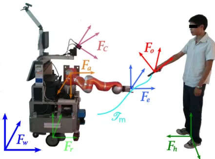
frame; Fa: robot base frame; Fc: camera frame; Fe: end effector frame; Fo: object frame; Fh: human frame. The trajectory Tmrealizing a manip-ulation should be successfully controlled in different task frames. Figure from [He 15]. . . 26 2.12 Left: trajectories of the control primitives. Right: trajectory switching for
the controller due to the movement of an obstacle. . . 26 2.13 A simple case of grasp. Left: a planned grasp defines contact points
be-tween the end effector and the object. Right: To finish the grasping, the manipulator must follow the blue trajectory P1- Pc, and then close the grip-per. This movement must be controlled in the object frame Fo. . . 28 2.14 In the left, each circle represents the controller of a control primitive. The
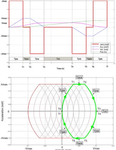
system can suspend or stop the execution of a control primitive. . . 30 3.1 The jerk evolution for the j axis of the T(t) trajectory. . . . 37 3.2 Jerk, acceleration, speed and position curves and motion in the
acceleration-velocity frame for a single axis.. . . 39 3.3 Example of the smoothing of a set function. . . 40
3.4 Way points motion: time synchronized, phase-synchronized and without
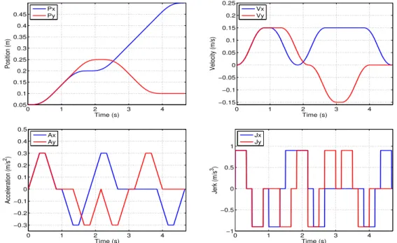
synchronization . . . 44 3.5 Position, velocity, acceleration and jerk profile of unsynchronized 2D
via-points motion. . . 45 3.6 Position, velocity, acceleration and jerk profile of time-synchronized 2D
via-points motion. . . 46 3.7 Position, velocity, acceleration and jerk profile of phase-synchronized 2D
via-points motion. . . 46 3.8 Influence of the start and end points for the smooth area . . . 47 3.9 Error between the smoothed trajectory and pre-planed path . . . 50 3.10 Smooth algorithm. (a) A jerky path as a list of waypoints. (b) Converting
into a trajectory that halts at each waypoints. (c) Performing a shortcut that fails in collision check. (d),(e) Two more successful shortcuts (f) The final trajectory. . . 53 3.11 (a) A collision-free C -space path covered by free bubbles. (b) 2D robot
ma-nipulator showing the maximum distance r1, r2 and the minimum obstacle
distance dobst. The circle at the axis of joint 1 of radius r1(the red dashed
line) contains the entire manipulator. The circle at joint 2 of radius r2 (the
3.12 A simulated move from an initial position to a final position with a static obstacle. (1) The purple dashed line is the first trajectory computed. (2) The robot detects an obstacle and plan a new trajectory. Note that the purple trajectory is in collision. (3) A new trajectory that avoid collision. (4) The complete trajectory realized in green. The green solid line is the real path, which the robot follows. By adding two waypoints, the robot reaches the
target position without collision and path replanning at the high level. . . . 58
3.13 The position, velocity, acceleration and jerk of online generated via-points trajectory on Z axis . . . 59
3.14 Paths of the robot end effector with different errors . . . 59
3.15 Left: A manipulator reaches under a shelf on a table from the zero position. Right: The blue curve depicts the original end effector path. The red curve depicts the smoothed path after 200 random shortcuts.. . . 60
3.16 Progression of the smoothing illustrated by the duration of the trajectory travelling for 10 initial paths for the same reaching task. The trajectories are relative to the task presented in Figure 3.15 . . . 61
3.17 The position, velocity, acceleration and jerk profile of the calculated trajec-tory in the robot reaching task . . . 61
3.18 The planning setup of the ICARO industrial scenario. Left: a global view of the setup. Right: the start configuration. . . 62
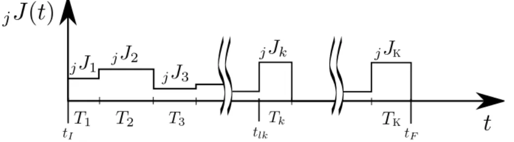
4.1 A trajectory is composed of K polynomial segments, tIand tFare the initial time and final time of the trajectory. . . 66
4.2 3rd degree polynomial interpolants with fixed time: the position, velocity, acceleration and jerk profiles. . . 67
4.3 3rd degree polynomial interpolants with fixed jerk . . . 68
4.4 Constraint type I of 4thdegree polynomial interpolants . . . . 70
4.5 Constraint type II of 4thdegree polynomial interpolants . . . 71
4.6 Constraint type III of 4thdegree polynomial interpolants . . . 72
4.7 One continuous interpolant with 5thdegree polynomial . . . 73
4.8 Four path samples to be approximated (unit: m) . . . 76
4.9 Comparison of characteristics for different approximations . . . 77
4.10 Top: computed motion law for the horse path; Middle: velocity error be-tween desired and computed motion law; Bottom: trajectory error bebe-tween the given trajectory and the approximated one. . . 78
4.11 Theoretical path, computed trajectory and the one recorded while the LWR arm is executing the computed horse trajectory. . . 79
5.1 Left: Joint usage in a car. Right: Mechanical structure of a joint . . . 83
5.3 The software architecture of ICARO project . . . 85 5.4 Two different gestures. (a) Validation: Validate the current operation, go to
the next task of the whole procedure. (b) Rebut: Reject the current operation. 85
5.5 The trajectory received the Command 2 and stopped the current motion at
around t= 3.8s. At the instant t = 13.8s, the Validation gesture was sent to trajectory controller so that it recover the previous movement. . . 86 5.6 Reactive planning structure. The input and output of each component is
de-tailed in this figure. Trajectory Monitor supervises the current robot motion and checks if future positions are in a collision state. In case of a coming collision, it requests a new path to the path planner. The new path is di-rectly sent to the trajectory generator and is converted into a new trajectory. The trajectory controller merges the current trajectory with the new one to obtain a smooth transition while avoiding the obstacles. . . 88 5.7 Aligning the outer shell using the force detection and a 3D printed part. . . 89 5.8 The position and force of the end-effector along the Z axis during the
posi-tioning task. . . 89 5.9 Force Fx, Fy, Torque Tx, Ty, Tz during the task. Measures are provided by
the FRI interface . . . 89 5.10 A human operator inserts balls into the RZEPPA joint. In picture (d), the
human uses one hand to open the joint and the other hand to insert the ball. 90 5.11 Sub-task of the insertion task of one ball. (a): Initial position. (b): Open
position. (c): Insertion position. (d): Closed position. . . 91 5.12 The structure of the Online Trajectory Generator based impedance controller. 91 5.13 The frames of the ICARO setup. Ft: the tool frame; Fe: the end-effector
frame; Fb: the robot base frame. . . 92 5.14 Real experiment of the ball insertion task with ICARO setup. (a): Initial
position. (b): The outer shell is aligned with the tool. (c): The robot moves to go to open position. (d): The operator places a ball in the gap. (e): The outer shell can hold the ball without the help of human. (f): The robot goes back to close the outer shell. It moves a bigger angle than step (c) to guarantee that the ball is fully enfolded by the outer shell. (g): The robot moves again to the aligned position and is ready to rotate for inserting the next ball. (h): Once all 6 balls are inserted successfully, the robot returns to the initial position. . . 94 5.15 Top: the force along the Z axis on the end-effector. Middle: the position
of the end-effector along the Z axis. Bottom: the received position and real position of joint 1.. . . 95
5.16 The hand of the human gets close to the outer shell when inserting a ball. If the robot moves unexpectedly at this moment, the human fingers may be injured. . . 96 5.17 Hands monitoring for safety . . . 96 6.1 Nonconstant motion constraints. The robot at the state M1 list in the red
constraints frame is going to transfer a new state. The states M2 and M3
locate in new constraints frames which are denoted as green and blue. The kinematics motion bounds (jJmax, jAmax, jVmax) are all changed. . . 101 A.1 Axis-Angle Representation . . . 104 C.1 Le robot manipulateur partage l’espace de travail avec un op´erateur humain
pour r´ealiser l’assemblage collaboratif d’un joint Rzeppa. L’illustration provient du projet ANR-ICARO. . . . 112 C.2 Le contrˆoleur de trajectoire se trouve `a un niveau interm´ediaire de l’architecture
du contrˆoleur, entre les contrˆoleurs rapides des axes du robots et le niveau planification plus lent.. . . 113 C.3 Influence du choix des points initiaux et finaux d´elimitant la zone liss´ee . . 116 C.4 Algorithme de lissage par raccourci. (a) La ligne polygonale initiale. (b)
Conversion en une trajectoire qui s’arrˆete `a chaque point de passage. (c) Une trajectoire plus courte en collision. (d-e) Deux trajectoires plus courtes r´eussies. (f) la trajectoire finale. . . 119
1
Introduction
1.1
Introduction
Interactive robots are now beginning to joint assembly and production lines. They com-plement the previous generation of robots, which were designed for performing operations quickly, repeatedly and accurately. They have now a long heritage in the manufacturing industry for operating in large numbers in relatively static environments. The development of traditional robotics in industry is confronted to the difficulty of programming and to the cost of safe guard designed to separate humans and robots. Due to the multiple advantages over a human operator, the arm manipulators, for example, have been used in various kinds of industrial applications, such as pick-and-place operations, welding, machining, painting, etc. The introduction of interactive robots simplifies the design of the production lines and the programming of robots.
Arm manipulator control for industrial applications has now reached a good level of maturity. Many solutions have been proposed for specific uses. However, all these applica-tions are confined to structured and safe spaces where no human-robot interacapplica-tions occur. With the growth of robotic presence in the human community, the need of intuitiveness in the human-robot interaction has become inevitable. The human-robot coexistence with var-ious degrees of restriction can be found in many areas, specifically in the industry services. There exist many tasks in the industrial scenarios where the robots (robotic arms) work to-gether with the humans. Therefore, it is necessary for the robots to interact smoothly and
intuitively to solve the task effectively, successfully and safely.
If robots could coexist with human workers, the robots could carry out monotonous and repetitive tasks with accuracy and at high-speed. Human workers could use their skills to do more complex tasks, such as assembly and preparation, post-processing tasks for the robots. This compensation of each other’s disadvantages holds promise for cooperation between human workers and robots. The concept of closeness is to be taken in its full meaning, robots and humans share the workspace but also share goals in terms of task achievement.
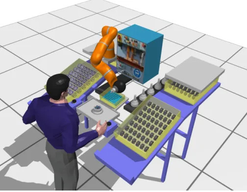
FigureC.1illustrates a scenario where a human operator cooperates with a KUKA LWR
arm manipulator to achieve an assembly task.
Figure 1.1: The robot manipulator shares the workspace with a human operator. They cooperate to assemble a Rzeppa Joint. Figure comes from the ANR Project ICARO
To realize robots working alongside humans in environments such as the home, at work, a hospital or any public place, the robots have to be safe, reliable and easy to use. In practice, the robot must guarantee the safety of humans when they share the same workspace, it is important to make the robot to avoid hurting humans during the operation even when an unexpected or not detected event occurs. The human’s comfort is another important aspect in robotic applications. In the context of human robot interaction, the robot should not cause excessive stress and discomfort to the human for extended periods of time [Lasota 14].
The two important approaches to define a robotic task are learning and motion planning. The learning approach uses different techniques to record a human-demonstrated motion or a skill, plans a task from these data and improves the execution of the task by learning,
such as Reinforcement Learning (RL) [Kober 13] and Learning from Demonstration (LfD) [?]. These approaches often represent the learned actions as trajectories. However, there are always unforeseen events in a dynamic environment. In this case the learning approaches are becoming less effective to adapt the produced trajectory to the context in real time, e.g. to grasp a moving object, or to avoid an obstacle.
The other way to define the robotic task is motion planning. Most of the motion planners define the motion by paths, which will be followed up by the robot. Unfortunately, the robot controller can only trace a small subset of these paths, but fails to follow up the majority of them efficiently and precisely. A better approach is to define motions more precisely using trajectories, which define the position as a function of time. We propose to introduce an intermediate level of control between the motion planner and the low level controller provided by the robot manufacturers. When the task is changing, e.g. by the presence of humans, planning new trajectories is necessary. In this case, a feedback from the controller describing its state and a trajectory describing the future state could be helpful to adapt the planned trajectory to the robot’s predicted state at the end of the next planning loop.
Moreover, motion planning is usually done off-line, especially when the trajectory gen-eration processes are computationally expensive. However, to perform a large variety of tasks autonomously and reactively, a robot must propose a flexible trajectory controller that can generate and control the trajectories in real time. To react to environment changes, the trajectory generation must be done online. Meanwhile, the robot needs to guarantee the human safety and the absence of collision. So the model for trajectory must allow fast computation and easy communication between the different components, including path planner, trajectory generator, collision checker and controller. To avoid replanning of an en-tire trajectory, the model must allow deforming locally a path or a trajectory. The trajectory controller must also accept to switch from an initial trajectory to follow to a new one.
1.2
Motivation
In a near future, robots are going to share workbench with humans, they even will work on the same workpiece together. Thus, the role of industrial robots is becoming a tool that engineers and technicians can interact with. Historically, robots used in industrial service are designed and programmed for relatively static environments. Anything unanticipated in the robot’s environment is essentially invisible, as the robot feedback is really limited (joint sensors for position and eventually torques). These primitive sensory capacities in most cases necessitate running robots in ‘work cells’, free from people and other changing elements. Once programmed, it is expected that the work environment the robot interacts with remain within a very narrow range of variance. Thus the robots are isolated in a physical as well as sensorial sense, little different from any number of dangerous, automated factory machines.
The motivation of this work can be expressed by an analogy: imagine that two human operators need to finish an assembly task together on a fabrication line. One of the operator A has to focus on the main construction task, while the other operator B is expected to prepare work sites, collect and deliver tools just as they are needed, or stabilize components during assembly. For industries or enterprises, it might be a lack of competitiveness in the modern business with expensive labor. So it is necessary to extend the capacity of the robots to enable the possibility for a robot to work with human and to assist humans. This thesis sets out to develop a robot that work side-by-side with human, i.e. the robot will assist the operator in the whole task. We propose to build a more flexible controllers that are needed to switch between different sensors and control laws, and thus to build a more reactive system. A part of the solution is to use trajectories to exchange information among the motion planner, the collision checker, the vision/force systems and the low level controller.
1.3
Research Objectives
The objective of this work is to build more reactive robots by introducing a trajectory con-troller as an intermediate layer in the software structure in the context of human-robot inter-action. Thus the controller should provide a method of generating smooth and time-optimal trajectories in real time. It also must be able to react to the environment changes. There-fore, the trajectory generation algorithm must be computationally simple. The trajectories must take into account the physical limitations of the robot, that is, not only the velocity limitation but also acceleration and jerk limitations.
This work aims to produce a trajectory controller that can not only accept any trajec-tory produced by a path planner, but also can approximate any types of trajectories. It will enlarge the type of paths that the robot can follow, which makes the robot competent in more complex tasks. The proposed trajectory controller, based on the concept of On-line Trajectory Generation (OTG), allows real time computation of trajectories and easy communication with the different components, including path planner, trajectory generator, collision checker and controller. The controller can also allow deforming locally a trajectory and accept to switch from an initial trajectory to a new trajectory to follow.
Moreover, the controller can accelerate/decelerate the robot on the main trajectory by changing the time function s(t). Imagine for example that a fast movement could cause some people anxiety when the robot is close to them. In this situation, the controller can still execute the task but only at a reduced speed. The time-scaling schemes can also be used to avoid dynamic obstacle while not changing the path of the robot.
A further objective is to apply this technique to sensor-based control. When the robot is able to build the dynamic model of the manipulated object, to track the movement of objects and human body parts, and to detect special events, it needs to finish the tasks while reacting to the movement or events. Based on the work of previous colleagues, we
propose a trajectory controller to achieve reactive manipulations. The controller integrates information from multiple sources, such as vision systems and force sensors, and use online trajectory generation as the central algorithm.
Trajectory Controller
Sensor data Actuators
ROBOT
q
Path Planner Trajectory planner PTP planner SmoothingTRs
Task Planner/supervisionlow level controller
x x
s(t)
Figure 1.2: Trajectory Controller as an intermediate layer in the software architecture, the servo system on robot is fast, while task planning and path planning are slow.
Figure C.2 illustrates the intermediate level in the software structure. The controller integrates information from other modules in the system, including geometrical reasoning and human aware motion planning. From the sensor information, the trajectory planner can generate non-linear time-scaling functions or replan new trajectories for reacting to the environment change. One advantage of our algorithm is to be more reactive to dynamically changing environments. A second advantage is the simplicity of the use of the controller.
1.4
Outline of this Manuscript
Following this introduction, this dissertation begins with the presentation of background and literature review on motion control, focusing on learning approach, path planning,
tra-jectory generation and reactive tratra-jectory control. Chapter 3 presents the tratra-jectory genera-tion problem, including straight-line trajectory generagenera-tion between waypoints, smooth near time-optimal trajectory generation. All these algorithms produce jerk-bounded motions. In Chapter 4, we present the trajectory approximation with polynomial functions. Chapter 5 focuses on the reactive trajectory controller, with the concept of control primitives and how it is used in human robot interactions. Following the three chapters, we give the discussion and conclusion, as well as the recommendation for future works in chapter 6. Because each chapter deals with a different problem, experimental results are given at the end of each chapter.
1.5
Publication, Software Development, and Research Projects
Publication during the thesis:
• RAN ZHAO, DANIEL SIDOBRE, Trajectory Smoothing using Jerk Bounded Short-cuts for Service Manipulator Robots, 2015 IEEE/RSJ International Conference on
Intelligent Robots and Systems (IROS), Hamburg, Germany, Sept. 28 – Oct. 02, 2015 (Accepted)
• RANZHAO, DANIELSIDOBRE ANDWUWEIHE, Online Via-points Trajectory Gen-eration for Reactive Manipulations, 2014 IEEE/ASME International Conference on
Advanced Intelligent Mechatronics (AIM), besanc¸on, France, 2014
• WUWEIHE, DANIEL SIDOBRE ANDRANZHAO, A Reactive Trajectory Controller for Object Manipulation in Human Robot Interaction, The 10th International
Con-ference on Informatics in Control, Automation and Robotics (ICINCO), Reykjavik, Iceland, 2013
• WUWEI HE, DANIEL SIDOBRE ANDRANZHAO, A Reactive Controller Based on Online Trajectory Generation for Object Manipulation, Lecture Notes in Electrical
Engineering, 159-176, Springer International Publishing
• DANIEL SIDOBRE, RAN ZHAO, Trajectoires et contrˆole des robots manipulateurs interactifs, Journ´ees Nationales de la Robotique Humano¨ıde, Nante, France, Jun.
2015
• RANZHAO, DANIEL SIDOBRE, Online Via-Points Trajectory Generation for Robot Manipulations, Congr`es des Doctorants EDSYS,2014
This work was partially reported in the ICARO project, which aims to developed tools to improve and to simplify the interaction between industrial robots on one side and humans and the environment on the other side. The author contributed to the development of several
software running on the robot kuka LWR, and maintenance of the robots. The author par-ticipated actively to the development of software and to the final integration for a research project:
• Project ICARO1, see Figure C.1. ICARO is a collaborative research project aiming to develop tools to improve and simplify interaction between industrial robots and humans and their environment. ICARO was funded by the program CONTINT of the ANR agency from 2011 to 2014.
The author participated in the development of several softwares:
• softMotion-libs: A C++ library for online trajectory generation. It can be tested in the
MORSE, the Modular OpenRobots Simulation Engine2.
• lwri-genom: A GenoM3 module for the trajectory generation of the KUKA LWR arm.
• lwrc-genom: A GenoM3 module for the trajectory control of the KUKA LWR arm. • coldman-genom: A GenoM3 module for the collision detection in robot
manipula-tion.
• pr2-softMotion: Genom interface for pr2-soft-controllers Most of the softwares listed above are accessible in robotpkg3.
1http://icaro-anr.fr/
2http://www.openrobots.org/wiki/morse/ 3http://robotpkg.openrobots.org/
2
Related Work and Background
2.1
Introduction
Service robots are becoming used to work in environments like home, hospitals and schools in the presence of humans. Therefore this expansion raises challenges on many aspects. Since the tasks for the robot to realize will not be predefined, they are planned for the new situations that the robots have to handle. Clearly, purely motion control with predefined trajectories will be not suitable for these situations. The robot should acquire the ability to react to the changing environment. Before presenting the main background of our de-velopments, several aspects need to be discussed and be compared to the state of the art: architecture for human-robot interaction, trajectory generation and control including online adaptation and monitoring. In this chapter, we will give a brief review of some foundation of the service robotic. Then we will survey the planning-based and learning-based techniques that are used for trajectory generation, followed by background material that motivates this research.
2.2
Software Architecture for Human Robot Interaction
The robots capable of doing HRI must realize several tasks in parallel to manage vari-ous information sources and complete tasks of different levels. Figure2.1shows the pro-posed architecture where each component is implemented as a GENOM module. GENOM
Figure 2.1: Software Architecture of the robot for HRI manipulation. Tmis the main tra-jectory calculated initially by MHP. The controller takes also costs from SPARK, which maintains a module of the environment. The controller sends control signals in joint (q in the figure) to the robot arm controller, and during the execution, the controller returns the state of the controller (s in the figure) to the supervisor
[Mallet 10a,Mallet 11] is a development environment for complex real time embedded soft-ware.
At the top level, a task planner and supervisor plan tasks as the output, such as cleaning the table, bring an object to a person and then supervises the execution. The module SPARK (Spatial Reasoning and Knowledge) maintains a 3D model of the whole environment, in-cluding objects, robots, posture and position of humans [Sisbot 07b]. It provides also the related geometrical reasoning on the 3D models, such as evaluating the collision risk be-tween the robot parts and bebe-tween the robot and its environment. An important element regarding SPARK is it produces cost maps, which describe a space distribution relatively to geometrical properties like human accessibility. The software for perception, from which SPARK updates the 3D model of the environment, is omitted here for simplicity. The mod-ule runs at a frequency of 20Hz, limited mainly by the complexity of the 3D vision and of the detection of human.
and grasp planner. RRT (Rapidly exploring Random Tree)[LaValle 01b] and its variants [Mainprice 10] are used by the path planner. The paths could be described in Cartesian or joint spaces depending on the task type. The output path of the planner is defined as a broken line. From this path, an output trajectory is computed to take the time into account. MHP calculates a new trajectory each time the task planner defines a new task or when the supervisor decides that a new trajectory is needed to react to the changes of the environment. When the motion adaptation is achieved by path replanning, the robot would switch between planning and execution, producing slow reactions and movements because of the time needed for the complex path planner. Furthermore, if object or human moves during the execution of a trajectory planned by the module MHP, the task will fail and so a new task or a new path needs to be planned. The human counterpart often finds the movement of the robot unnatural and so not intuitive to interact with.
Motor Controller Trajectory Controller Motion Planner
Figure 2.2: Trajectory Controller is introduced as an intermediate layer in the software architecture, between the low level and fast motor controller and the high level planner, which is slow.
2.3
Trajectory Generation
Trajectory generation computes the time evolution of a motion for the robot. Trajectories can be defined in joint space or in Cartesian space. They are then directly provided as the input for the controller. Trajectories are important because they enable the system to ensure: • feasibility: the motion can be verified to respect the dynamic constraints of
lower-level controllers.
• safety and comfort: the trajectories can limit velocity, acceleration and jerk, which are directly related to the safety and comfort for humans.
Space of defination Task type Path geometry Timing law Synchronization Cartesian trajectory Joint trajectory Point to point (PTP) Multiple points Bang-bang in acceleration Trapezoidal in velocity Polynomial Coordinated Independent Dimension Monodimensional Multidimensional
}
}
}
}
}
}
... Rectilinear CycloidPolynomial ... Continous ConcatenatedFigure 2.3: Categories of trajectories [Siciliano 08b]
• optimization: optimization can integrate both geometry and time.
• flexibility: trajectories allow to define a lot of tools to adapt and transform them.
2.3.1 Trajectory Types
Siciliano proposed classifications to verify trajectories [Siciliano 08b] (Figure2.3). From spatial point of view, trajectories can be planned in joint space or Cartesian space. Joint space trajectories have several advantages:
• Trajectories planned in joint space can be used directly to control low-level motors without need to compute inverse kinematics.
• The dynamic constraints, like maximum acceleration on joints, can be considered while generating the trajectories. On the contrary, these constraints should be tested after inverse kinematic for Cartesian space trajectories.
Cartesian space trajectories are directly related to task properties, allowing a more direct visualization of the generated path. Generally, they produce more natural motions, which are more acceptable results for people. For a simple motion like hand over an object, a trajectory planned in Cartesian space can produce a straight-line movement, which is not easy to guarantee while planning in joint space. The advantage of Cartesian space planning is also evident for task constraints. For example, when the robot needs to manipulate a cup of tea without spilling it out.
From another point of view, a motion can be completed by the choice of different timing laws s(t) along the same path P.
T(t) = P(s(t)) (2.1)
where T(t) is the trajectory. If s(t) = t, the path is parameterized by the natural time. The timing law is chosen based on task specifications (stop in a point, move at constant velocity, and so on). It also may consider optimality criteria (min transfer time, min energy, . . . ). Constraints are imposed by actuator capabilities (max torque, max velocity, . . . ) and/or by the task (e.g., max acceleration on payload).
Trajectories might also be classified as coordinated trajectories or independent trajec-tories, according to the synchronization property. For coordinated trajectories the motions of all joints (or of all Cartesian components) start and end at the same instant. It is equiv-alent that all joints have the same time law. While independent trajectories are timed in-dependently according to the requested displacement and robot capabilities. This kind of trajectory exists mostly only in joint space.
From another point of view, Biagiotti [Biagiotti 08] proposed a classification based on the dimension and task type, as shown in Figure2.4. Mono-dimensional trajectories cor-respond to trajectories for systems of only one degree of freedom (DOF), while
Multi-dimensionalfor more than one DOF. Compared to the case of mono-dimension, the diffi-culty for multi-dimensional trajectories is the synchronization of the different axis. A point-to-point trajectories simply link two points, while a multi-points trajectories pass through all points in the middle. Trajectory approximation and interpolation are usually used when we get movement data from a set of measured locations at known times. In general, trajectory interpolation of locations defines the velocity.
These trajectories are usually long-term trajectories as there is some distance between each waypoints provided by a motion planner. A trajectory can also connect two different trajectories. When the robot is moving along a trajectory and receiving a request to switch to another trajectory, generation of a connection trajectory can allow the robot to joint up smoothly the new trajectory. In this case, the trajectory links two robot states of non-null
velocities and/or accelerations.
Figure 2.4: Classification of trajectories based on dimension and task type [Biagiotti 08]
2.3.2 Trajectory Generation Algorithms
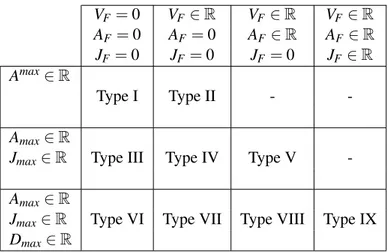
Trajectory generation for manipulators have been discussed in numerous books and papers, among which readers can find [Brady 82], [Khalil 99] and [Biagiotti 08]. Kroger, in his book [Kroger 10b], gives a detailed review on on-line and off-line trajectory generation. He proposes a classification based on the complexity of the generation related to the number of constraints, as in table2.1[Kroger 10b]. From any situation, Kr¨oger proposes to reach a goal defined by constraints (position, velocity, acceleration, jerk, . . . ) while respecting bounds (Vmax, Amax, Jmax, Dmax, . . . ). Vmaxis the maximum velocity, Amax is the maximum acceleration, Jmax is the maximum jerk, Dmaxis the maximum derivative of jerk. The defi-nitions presented in this table are used in this document.
2.3.2.1 Robot Motion Representation
We firstly consider the kinematics of a rigid body in a 3D space. Considering a reference frame, Fw, which can be defined as an origin Ow and an orthogonal basis(Xw,Yw, Zw). A rigid body B is localized in 3D space by a frame FB, as shown by Figure2.5.
Translations and rotations shall be used to represent the relation between these two frames. For the translation, Cartesian coordinates are used, but for rotations, several choices are available:
• Euler rotations • Rotation matrices • Quaternions
Figure 2.5: Rigid body localization in 3D space
The homogeneous transformation matrix is often used to represent the relative displacement between two frames in computer graphics and robotics because it allows common opera-tions such as translation, rotation, and scaling to be implemented as matrix operaopera-tions. The displacement from frame FW to frame FBcan be written as:
TFB FW = x R3×3 y z 0 0 0 1 (2.2)
In which, R3×3 is the rotation matrix and[x, y, z]T represents the translation. Given a point
bwhich is localized in local frame FB:
BP
b= [xbybzb1]T
And TFW
FB represents the transformation matrix between frame FB and FW, then the position
of point b in frame FW is given as:
WP
b= TFFWBBPb
If a third frame is given as FD, the composition of transformation matrix is also directly given as: TFD FW = T FB FWT FD FB
Other representations used in this thesis are quaternion and Euler axis and angle, the de-tails of which is given in Appendix. Readers can also refer to the literature such as the book of Siciliano [Siciliano 08a] for more comparison and discussion on different types of representations for rotations and translations.
2.3.2.2 Online Trajectory Generation (OTG)
A large work is relative to off-line trajectory generation in the literature. A general overview of basic off-line trajectory planning concepts is presented in the textbook of Khalil and Dombre [Khalil 99]. Kahn and Roth [M.E 71] belong to the pioneers in the field of time-optimal trajectory planning. They used methods of time-optimal, linear control theory and achieved a near-time-optimal solution for linearized manipulators. The work of Brady [Brady 82] introduces several techniques of trajectory planning. In later works, the ma-nipulator dynamics were taken into account [Bobrow 85], and jerk-limited trajectories were applied [Kyriakopoulos 88]. The concept of Lambrechts et al. [Lambrechts 04] produces very smooth fourth-order trajectories but is also limited to a known initial state of motion and to one DOF. As the thesis tries to achieve reactive robot control, only on-line generation is suitable for the trajectory control level.
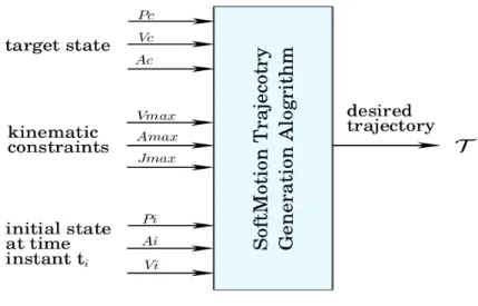
We first introduce the concept of the Online Trajectory Generation. A first OTG algo-rithm is able to calculate a trajectory at any time instant, which makes the system transfer from the current state to a target state. Figure2.6illustrates the input and output values of OTG algorithm. The trajectory generator is capable of generating trajectories in one time cycle. The usage of an online trajectory generation algorithm may have two main reasons:
• The first reason is that the trajectory can be adapted in order to improve the path accu-racy. [Dahl 90] proposed to use one-dimensional parameterized acceleration profiles along the path in joint space instead of adapted splines. [Cao 94, Cao 98] used cu-bic splines to generate smooth paths in joint space with time-optimal trajectories. In this work, a cost function was used to define an optimization problem consider-ing the execution time and the smoothness. [Constantinescu 00] suggested a further improvement of the approach of [Shiller 94] by leading to a limitation of the jerk in joint space, considering the limitation of the derivative of actuator force/torques. [Macfarlane 03] presented a jerk-bounded, near time-optimal, one-dimensional tra-jectory planner that uses quintic splines, which are computed online. Owen published a work on online trajectory planning [Owen 04]. Here, an off-line planned trajectory was adapted online to maintain the desired path. The work of Kim in [Kim 07] took robot dynamics into account.
• The other one is the robotic system must react to unforeseen events based on the sen-sor singles when the robot works in an unknown and dynamic environment. [Castain 84] proposed a transition window technique to perform transitions between two different path segments. [Liu 02a] presented a one-dimensional method that computes linear acceleration progressions online by parameterizing the classic seven-segment acceler-ation profile. [Ahn 04] used sixth-order polynomials to represent trajectories, which is named Arbitrary States POlynomial-like Trajectory (ASPOT). In [Chwa 05], Chwa presented an advanced visual servo control system using an online trajectory planner
Figure 2.6: Input and output values of the Online trajectory generation algorithm. P: Posi-tions, V : Velocities, A: Accelerations
considering the system dynamics of a two-link planar robot. An algorithm proposed in [Haschke 08a] is able to generate jerk-limited trajectories from arbitrary state with zero velocity. Broqu`ere proposed in [Broquere 08] an online trajectory planner for an arbitrary numbers of independent DOFs. This approach is strongly related to a part of this thesis.
Some approaches to build a controller capable of controlling a complete manipulation tasks are based on Online Trajectory Generation. More results on trajectory generation for robot control can be found in [Liu 02b], [Haschke 08b], and [Kr¨oger 06]. Kr¨oger proposed an algorithm to generate type IV trajectories in table2.1. Broqu`ere et al. ([Broquere 08]) proposed type V trajectories, with arbitrary final velocity and acceleration. The difference is important when the controller needs to generate trajectories to join points with arbitrary velocity and acceleration. This is the case to follow a trajectory using an external sensor.
2.3.3 Planning-based Trajectory Generation
We present firstly basic notions for planning in presence of geometrical constraints for Hu-man Robot Interaction. Then we discuss the motion of a rigid body in space, before we introduce the motion planning techniques and control laws for the robot manipulators.
2.3.3.1 Geometrical Constraints in HRI
The presence of humans in the workspace of a robot imposes new constraints for the motion planning and the control for navigation and manipulation. This field has been intensively studied especially at LAAS-CNRS. The more important constraints are relative to the
se-VF = 0 VF ∈ R VF ∈ R VF ∈ R AF = 0 AF = 0 AF ∈ R AF ∈ R JF = 0 JF = 0 JF= 0 JF ∈ R Amax∈ R Type I Type II - -Amax∈ R
Jmax∈ R Type III Type IV Type V
-Amax∈ R
Jmax∈ R Type VI Type VII Type VIII Type IX
Dmax∈ R
Table 2.1: Different types for on-line trajectory generation. VF: final velocity, AF: final acceleration, JF: final jerk.
curity, the visibility and the comfort of human counterpart, two of these constraints are illustrated in Figure2.7.
For robot motion, the workspace could be associated with many cost maps, each com-puted for a type of constraint. The first costmap is comcom-puted mainly to guarantee the safety and security of people at motion planning and robot control level by considering the dis-tance to dangers. In this case, only disdis-tances are taken into consideration. This constraint keeps the robot far from the head of a person to prevent possible dangerous collision be-tween the robot and the person. The theory from [Hall 63] shows that the sensation of fear is generated when the threshold of intimate space is passed by other people, causing inse-curity sentiments. For this reason, the cost near a person is high while tends towards zero when the distance becomes high.
The second constraint is called visibility, this is to limit firstly the surprise effect to a person while robot is moving nearby, secondly, a person feels less surprised when the robot is moving in the visible zone, and feels more comfortable and safe [Sisbot 07a]. For example, when the robot hand over an object, this constraints can verify that the person is paying attention to the object exchange.
Other constraints are also used, which can be found in [Sisbot 07a] and related publica-tions. For example, while planning a point in space to exchange an object, this point should be reachable by the person, computed by the length of his arm and the possibility to produce a comfortable posture for the person. A cost of comfort is also computed for every human posture [Yang 04].
When all the cost maps are computed, they are combined in the global cost c(h, x):
c(h, x) = N
∑
i=1
wici(h, x)
which the cost maps are computed. wi is the weight. This combined cost map is used during the motion planning. In this thesis, we proposed to use it to modulate the velocity at the trajectory control level.
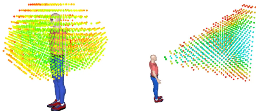
Figure 2.7: Left: 3D reachability map for a human. Green points have low cost, meaning that they are easier for the human to reach, while the red ones, having high cost, are difficult to reach. One application is that when the robot plans to give an object to a human, an exchange point must be chosen in the green zone. Right: 3D visibility map. Based on visibility cost, the controller can suspend the execution if the human is not looking at the robot.
2.3.3.2 Path Planning
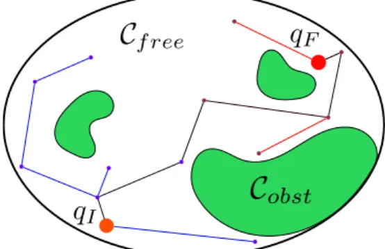
Through this thesis, the robot is assumed to operate in a three-dimensional space (R3), called the work space (W ). This space contains many obstacles, which are rigid bodies, written as W Oi, i means it is the ith obstacle. And the free space is then Wf ree = W \SiW Oi, where\ is the set subtraction operator. Motion planning can be performed in working space or in configuration space Q, called C-space (Figure2.8). C-Space is the set of all robot configurations. Joint space is often used as C-space for manipulators. Configurations are often written as q1. The obstacles in the configuration space correspond to configurations where the robot is in collision with an obstacle in the workspace.
A path is a continuous curve from the initial configuration (qI in Figure. 2.8) to the final configuration (qF in Figure. 2.8). It can be defined in the configuration space or in the workspace (planning in Cartesian space). Path is different from trajectory such that trajectories are functions of time while paths are functions of a parameter. Given a parameter
u∈ [umin, umax], often chosen such that u ∈ [0,1], a path in configuration space is defined as a curve P such that:
P :[0, 1] → Q where P(0) = qI, P(1) = qF and P(u) ∈ Qf ree, ∀u ∈ [0,1] (2.3)
Figure 2.8: Configuration Space and a planned path in C space from qIto qF.
Path planning has been one of the essential problems to solve in robotics. Among nu-merous papers and books, chapter V of Handbook of Robotics, by Kavraki and La Valle [Kavraki 08] provides an introduction to this domain, and the book of LaValle [LaValle 06] provides numerous methods. For this work, we selected the large class of planners that pro-vide the output path in the form of via-points. Figure2.9shows an example of the result of a path planning, which gives a series of waypoints in the configuration space, linking points
qIand qF.
Figure 2.9: Results of path planning (by diffusion) as a series of points in the configuration space. The resulting path is in black.
When the robot shares the workspace with humans, the path planner must take into account the costs of HRI constraints. We perform this planning with the T-RRT method [Jaillet 10] which takes advantage of the performance of two methods. First, it benefits from the exploratory strength of RRT-like planners [LaValle 01a] resulting from their ex-pansion bias toward large Voronoi regions of the space. Additionally, it integrates features of stochastic optimization methods, which apply transition tests to accept or reject poten-tial states. It makes the search follow valleys and saddle points of the cost-space in order to compute low-cost solution paths (Figure.2.10). This planning process leads to solution paths with low value of integral cost regarding the costmap landscape induced by the cost function.
per-Figure 2.10: T-RRT constructed on a 2D costmap (left). The transition test favors the exploration of low-cost regions, resulting in good-quality paths (right).
turbation variant described in [Mainprice 11] are usually employed. In the latter method, a path P(s) (with s ∈ R+) is iteratively deformed by moving a configuration qperturb ran-domly selected on the path in a direction determined by a random sample qrand. This process creates a deviation from the current path, the new segment replaces the current segment if it has a lower cost. Collision checking and kinematic constraints verification are performed after cost comparison because of the longer computing time.
The path P(s) computed with the human-aware path planner consists of a set of via-points that correspond to robot configurations. Via-via-points are connected by local paths (straight line segments). Additional via-points can be inserted along long path segments to enable the path to be better deformed by the path perturbation method. Thus each local path is cut into a set of smaller local paths of maximal length lmax.
2.3.4 Learning-based Trajectory Generation
Here we present a brief overview of methods for motion generation based on observing and repeating sample motion trajectories. Unlike the planning and control methods we presented so far, imitation learning methods make no assumption that a cost function spec-ifying desired motions exists. Rather, the challenge is to learn approximate models (e.g. with machine learning) of this cost using the available data that can be used to generate motion.
2.3.4.1 Direct Policy Learning
Direct Policy Learning (DPL) is one of the fundamental approaches for imitation learning, see [Pomerleau 91,Argall 09]. Sometimes it is also called “behavior cloning”, because it is a straightforward approach that tries to repeat observed motions.
A standard way to describe a robot trajectory is{xt, ut}tT = 0, where xt represents the robot state at time t and ut is the control signal, e.g. the rate of change ˙xt. DPL tries to find a policy π : xt 7−→ ut from these observations. Different assumptions can be made for the choice of x, u and π [Calinon 07], with refinements like data transformations and
active learning. Given a parameterization of the policy, DPL essentially corresponds to a regression problem, e.g. with loss:
Ed pl= T
∑
t=0
kπ(xt) − utk2 (2.4)
wherek.|2demotes the squared L2norm. Minimizing Ed pl finds a policy close in the least squares sense to the demonstrations. The above loss can be extended to multiple demon-stration trajectories by averaging over them.
Howard et. al [Howard 09] introduces an interesting alternative loss for DPL:
Ed pl= T
∑
t=0
(kutk − π(xt)Tut/kutk)2 (2.5)
This loss penalizes the discrepancy between the projection of the policyπ(xt) on utand the true control ut . This article shows that in some problem domains this loss leads to better behavior than the standard least squares loss.
When the state and control spaces are high dimensional, DPL has a disadvantage: Gen-eralization is an issue and would essentially require the data to cover all possible situations.
2.3.4.2 Markov Decision Process and Reinforcement Learning
A Markov Decision Process (MDP) is a graphical model involving world states (e.g. robot position) and actions a (e.g. go left). It is a popular formalism for multiple learning prob-lems, including Reinforcement Learning (RL), see [Russell 09]. The MDP is defined by the following probabilities, taken for reference from [Jetchev 11]:
• world’s initial state distribution P(s0) • world’s transition probabilities P(st+1|at, st)
• world’s reward probabilities P(rt|at, st) and R(a, s) := E{|a,s} • agent’s policyπ(at|st) = P(a0|s0;π)
The value (expected discounted return) of policyπ when started in state s with discount-ing factorγ∈ [0,1] is defined as:
Vπ(s) = Eπ{r0+ γr1+ γ2r2+ . . . |s0} (2.6)
One way to do reinforcement learning in a MDP is to iterate the Bellman optimality equation until convergence of the value function - Value Iteration algorithm [Bellman 03]:
V∗(s) = max
a [R(a, s) + γ
∑
s′
The optimal policy given the optimal value function is simply the policy maximizing the immediate reward and expected future rewards:
π∗(s) = arg max
a [R(a, s) + γ
∑
s′
P(s′|a,s)V∗(s′))] (2.8)
The value of a state V(s) is a more global indicator of desired states than the immediate reward of an action R(a, s). The values V (s) provides a gradient towards the desired states-going in direction of increasing V(s) is the desired behavior of the robot system.
2.3.4.3 Inverse Optimal Control
Reinforcement learning or planning in general (e.g. within a MDP framework) tries to generate motions maximizing some reward. Learning (e.g. with Value Iteration) requires constant feedback in the form of rewards for the states and action of the agent. However, in many tasks the reward is not analytically defined and there is no way to access it from the environment accurately. It is then up to the human expert to design a reward leading the robot to the desired behavior. There is an algorithm that can effectively learn the desired behavior and a policy for it just by observing example motions. Inverse Optimal Control (IOC), also known as Inverse Reinforcement Learning (IRL), aims to limit the reward feed-back requirement and human expertise required to design behavior for a task. IOC learns a proper reward function only on the basis of data, see [Ratliff 06]. Let’s assume that policies π give rise to expected feature counts ϖ(π) of feature vectors φ : i.e. what feature we will see if this policy is executed. A weight vectorω such that the behavior demonstrated by the expertπ∗ has higher expected reward (negative costs) than any other policy is learned by minimizing a loss:
min|ω|2 (2.9)
s.t. ∀π ωTϖ(π∗) > ωTϖ(π) + L (π∗, π) (2.10)
The termωTϖ(π) defines an expected reward, linear in the features. The scalable margin L penalizes those policies that deviate more from the optimal behavior ofπ∗. The above loss can be minimized with a max margin formulation. Efficient methods are required to find the π that violates the constraints the most and add it as new constraint. Once the reward model is learned, another module is required to generate motions maximizing the reward, e.g. [Ratliff 06] uses an A∗planner to find a path to a target with minimal costs.
Learning a policy based on estimated costs is much more flexible than DPL, and a simple cost function can lead to complex optimal policies. IOC can often generalize well to new situations, because states with low costs create a task manifold, a whole space of desired robot positions good for the task. In some domains it is much easier to learn a mapping from state to cost than to learn a mapping from state to action. The latter is a
more complex and higher dimensional problem, especially when considering actions in high dimensional continuous spaces such as robot control.
2.3.4.4 Discriminative Learning
Discriminative learning provides a common framework for many learning problems, in-cluding structured output regression. Popular approaches include large margin models [Tsochantaridis 05] and energy based models using neural networks [Lecun 06]. Data is given in the form of pairs of input and output values{xi,yi}. As in standard discriminative approaches (e.g., structured output learning), the energy or cost f(xi, yi;ω) provides a dis-criminative function such that the true output should get the lowest energy from the model
f:
yi= arg min
y∈y
f(xi, y) (2.11)
Training the parameter vectorω of the model f is done by minimizing a loss over the dataset. The loss should have the property that f is penalized whenever the true answer
yihas higher energy than the false answer with lowest energy which is at least distance r away:
yi= arg min y∈yky−yik>r
f(xi, y) (2.12)
Finding the most offending answer yiis very often a complicated inference problem in itself.
2.4
Robot Motion Control
Firstly, trajectory generation based approaches were developed. In [Buttazzo 94], results from visual system pass firstly through a low-pass filter. The object movement is modeled as a trajectory with constant acceleration, based on which, catching position and time is estimated. Then a quintic trajectory is calculated to catch the object, before being sent to a PID controller. The maximum values of acceleration and velocity are not checked when the trajectory is planned, so the robot gives up when the object moves too fast and the maxi-mum velocity or acceleration exceeds the capacity of the servo controller. In [Gosselin 93], inverse kinematic functions are studied, catching a moving object is implemented as one application, a quintic trajectory is used for the robot manipulator to joint the closest point on the predicted object movement trajectory. The systems used in those works are all quite simple and no human is present in the workspace. A more recent work can be found in [Kr¨oger 12b], in which a controller for visual servoing based on Online Trajectory Genera-tion (OTG) is presented. The results are promising.
![Figure 2.4: Classification of trajectories based on dimension and task type [ Biagiotti 08 ]](https://thumb-eu.123doks.com/thumbv2/123doknet/2180771.10499/34.892.150.742.207.454/figure-classification-trajectories-based-dimension-task-type-biagiotti.webp)