HAL Id: hal-03195346
https://hal.archives-ouvertes.fr/hal-03195346
Preprint submitted on 11 Apr 2021
HAL is a multi-disciplinary open access
archive for the deposit and dissemination of
sci-entific research documents, whether they are
pub-lished or not. The documents may come from
teaching and research institutions in France or
abroad, or from public or private research centers.
L’archive ouverte pluridisciplinaire HAL, est
destinée au dépôt et à la diffusion de documents
scientifiques de niveau recherche, publiés ou non,
émanant des établissements d’enseignement et de
recherche français ou étrangers, des laboratoires
publics ou privés.
Performance evaluation of feature selection and
tree-based algorithms for traffic classification
Ons Aouedi, Kandaraj Piamrat, Benoît Parrein
To cite this version:
Ons Aouedi, Kandaraj Piamrat, Benoît Parrein. Performance evaluation of feature selection and
tree-based algorithms for traffic classification. 2021. �hal-03195346�
Performance evaluation of feature selection and
tree-based algorithms for traffic classification
Ons Aouedi, Kandaraj Piamrat and Benoˆıt Parrein
University of Nantes, LS2N (UMR 6004) 2 Chemin de la Houssini`ere BP 92208, 44322 Nantes Cedex 3, France
{firstname.lastname}@ls2n.fr
Abstract—The rapid development of smart devices triggers a surge in new traffic and applications. Thus, network traffic classification has become a challenge in modern communications and may be applied to a various range of applications ranging from QoS provisioning to security-related applications. Devel-oping Machine Learning (ML) methods, which can successfully distinguish network applications from each other, is one of the most important tasks. Since ML algorithms are as good as the quality of data, feature selection has become a crucial step in the ML process. Therefore, selecting effective and relevant features for traffic analysis is also another essential issue. In this paper, we are interested in identifying the most relevant features to characterize network traffic. Empirical results indicate that significant input feature selection is important to classify network traffic. Then, a comparative analysis of various Decision Tree-based models (both traditional and recent algorithms) has been conducted with feature selection methods in terms of accuracy, training, and classification time.
Index Terms—Feature selection, traffic classification, machine learning, autonomous network, ensembles learning, CatBoost, XGBoost, LightGBM, Random Forest.
I. INTRODUCTION
Traffic classification is a basic requirement for providing a good Quality of Service (QoS) in network management. QoS represents the ability to provide different priority requirements to different traffic types. To do so, network operators need to identify and classify different types of traffic. Machine Learning (ML) can be efficient for that since it can build com-puter programs that automatically enhance their performance by experience [1]. Accordingly, ML is a promising solution to provide us a powerful and automatic traffic classification (both in terms of accuracy and speed). It started to flourish with net-work management, through the use of the centralized control capabilities provided by Software-Defined Networking (SDN). Several researchers argue that with the arrival of SDN, there is a high potential for collecting data from forwarding devices, which need to be handled by ML due to their complexity. Thus, combining real network data and machine learning with the benefits of SDN is still an open research area. The main issue is that a real dataset can have redundant (feature with predictive ability covered by another) and irrelevant (feature that provides no useful information) features, which increase search space and decrease predictive quality [2].
The time complexity of many ML algorithms is polyno-mial in the data dimensions [3] and SDN is a time-critical
system. Thereby, in classification domains, some features can hinder the classification process, where the increase in the data dimensionality may decrease the predictive ability of an algorithm as well as cause an extra computational cost (e.g., storage and processing) [4]. Consequently, in order to perform a more focused and faster analysis, feature selection can be used to create an efficient model.
Moreover, several classification algorithms are being ex-plored continuously by researchers. Despite the fact that Decision Tree (DT) has been successfully applied in traffic classification related studies [5]; from a large body of litera-ture, there is a lack of research comparing the performance of several DT-based models (both traditional and recent ones) for network traffic classification based on the same data set. Inspired by the discussion above and to eliminate this gap in the literature, a comparative evaluation is necessary. In brief, the major contributions of this paper are listed as follows:
• Dimensinality Reduction: In an offline manner, we have
applied two feature selection methods in order to find significant features from the entire dataset. In particular, we have used correlation filtering to delete the redundant features. Then, a comparative analysis of Information Gain Attribute Evaluation (IG) and Recursive Features Elimination (RFE) has been conducted. The selected optimal subspace, which represents the lower dimensional features, is then used in the training and testing phases of several classifiers.
• Empirical study of ML techniques: To provide useful insights for researchers into the behavior of several ML algorithms in traffic classification, we have selected six representative and well-known Tree-based classifiers. These classifiers are Random Forest (RF), Decision Tree (DT), adaptive boosting (Adaboost), and the novel Boost-ing algorithms, which are eXtreme Gradient BoostBoost-ing (XGBoost); as well as two recent classifiers such as CatBoost and Light Gradient Boosting Machine (Light-BGM). The performances of the resulting models were evaluated using accuracy, training, and classification time with the use of both default and tuned hyper-parameters. The rest of the paper is organized as follows. Section II pro-vides related works while Section III introduces our method-ology for feature selection and supervised learning algorithms
used for network traffic classification. Then, Section IV and Section V present the dataset used during this work and discuss the details of the experiments and their corresponding results. Finally, conclusions are summarized in Section VI.
II. RELATED WORK
Based on continuous changes in the behaviors of the appli-cations, several approaches have been proposed and used over the years. In this section, we provide a brief overview of some representative network traffic classification approaches. A. Traditional approaches
Port-based classification is the most simple technique. How-ever, it has some limitations, for example, applications can use dynamic port number or ports associated with other protocols to hide from network security tools [6]. To avoid total reliance on the semantics of port numbers, the DPI technique has been proposed to inspect the payload of the packets searching for patterns that identify the application. It checks all packets data, which consumes a lot of CPU resources and can cause a scalability problem. Moreover, it fails to classify encrypted traffic [7].
Due to the complexity of network application behaviors, these techniques are becoming inefficient solutions for traffic classification. In this context, ML is used as an alternative approach to classify the traffic by exploiting different char-acteristics of applications (i.e., features). As a result, a vast number of machine learning approaches have been used to classify traffic.
B. ML-based traffic classification
In [8], two feature selection methods have been used for traffic classification followed by six supervised learning methods (Naive Bayes, Bayes Net, Random Forest, Decision Tree, Naive Bayes Tree, and Multilayer Perceptron). Similarly, the authors in [9] present a comparative analysis of four supervised ML models for network traffic classification, which are Decision Tree (C4.5), SVM, BayesNet and NaiveBayes. However, these works does not include any of the boosting algorithms. Moreover, the authors in [10] have used Deep Learning (DL) as semi-supervised learning for network traffic classification with the help of dropout and denoising code hyparameters in order to improve the classification per-formance. However, DL has many hyper-parameters and their number grows exponentially with the depth of the model. Therefore, finding suitable architecture (i.e. number of hidden layers) and identifying optimal hyper-parameters (i.e. learning rate, loss function, etc.) are difficult tasks. Also, the authors in [11], proposed an architecture to classify network traffic with SDN, using unsupervised and supervised ML approaches. To avoid manual labeling of data, K-Means has been used to label the dataset. Then, several supervised learning methods are trained and evaluated individually, which are SVM, Deci-sion Tree, Random Forest, and KNN. However, the features used for clustering and classification are selected manually.
There could be found an expanding body of literature about using tree-based learning algorithms in traffic classification. However, there are new classification methods (e.g., CatBoost, LightGBM, etc.) that are not yet applied to this field. Also, it can be noticed that many works have been investigated using ML for network traffic classification; however, most of them used some specific classifiers and no one explores the DT-based classifiers (i.e., bagging and boosting together) using real network dataset.
III. METHODOLOGY
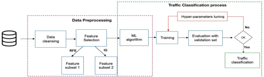
Figure 1 describes the methodology followed in this study, which includes two main processing steps: (i) data prepro-cessing and (ii) traffic classification. In this context, various methods of feature selection followed by the classification have been conducted. These methods are presented below. The last step consists of performance evaluations of the classification using accuracy, training and classification time. A. Data Preprocessing
Data preprocessing is a data mining technique that is used to transform the data and make it suitable for another processing use (e.g. classification, clustering). It is a preliminary step that can be done with several techniques among which data cleaning and feature selection.
1) Data cleaning: When the dataset has several features of different types but some ML models can only work with nu-merical values, it is necessary to convert or reassign nunu-merical values. In this work, we have converted the initial values of timestamp and IP address to numerical values. Also, as the dataset consists of different features with values on different scales, it needs to be scaled. This can be done by Min-Max normalization to perform features scaling. It is a technique that scales every feature of our dataset between 0 and 1, the maximum value of that feature gets transformed to 1 and the minimum value gets transformed to 0.
2) Feature Selection: One of the contributions of this paper is to find the optimum number of features (F ) that can provide the best classification performance in a real dataset. To do so, we have used features selection methods to identify the best features set in the offline run. Features selection methods try to pick a subset of features that are relevant to the target concept and have become an indispensable component of the ML process. There are many benefits of feature selection such as (i) defying the curse of dimensionality to improve the performance of learning algorithms either in terms of learning speed and generalization capacity, and (ii) reducing the storage requirement [12]. In fact, feature selection is a difficult task not only because of the huge size of the initial dataset but because it needs to maximize the learning capacity and to reduce the number of features.
To solve these problems, one of the purposes of this work is to select the relevant features for classification. This process can be defined as finding a minimal subset of feature F that maximizes the performance of ML model M () according to evaluation metric P (i.e., accuracy). Consequently, in this
Fig. 1. Structure of the experimental methodology
paper, feature selection strategies are implemented by two phases: correlation filtering and features selection.
- Correlation filtering is used to remove the redundant features and hence reduce the over-fitting of the classifiers as well as decrease the complexity of computation. It uses the correlation coefficient that indicates the linear correlation between two random features (i.e., variables) fi and fj.
The values of correlation cor range from −1 to 1. Usually, if |cor| > 0.5, this means that fiand fjhave a strong correlation;
if |cor| is close to 0, means that there is no linear correlation between the features. In fact, features are usually designed with their unique contributions, and removing any of them may affect the training accuracy to some degrees [13]. That is why we have deleted just the redundant features. In other words, we deleted every one of two features that have a correlation |cor| = 1, which means that they are totally redundant.
-Feature selection is intended to find the features that can help the classifier to distinguish better among the applications (target variable). We have used Information Gain Attribute Evaluation (IG) as the filter method [14], which is one of the widely used method [15]. The main concept of this approach is to rank subsets of attributes by calculating the IG entropy for each attribute in decreasing order. Each attribute gains a score from 1 (most relevant) to 0 (least relevant). The entropy of Y (target variable) is:
H(Y ) = −X
y∈Y
p(y) log2(p(y)) (1)
Then, IG measures the mutual information provided by X on Y.
IG = H(Y ) − H(Y /X) = H(X) − H(X/Y ) (2) Also, we used Recursive Features Elimination (RFE) [16] that recursively evaluates alternative sets by running some in-duction algorithms on the training data and using the estimated accuracy of the resulting classifier as its metric. Starting from all the feature sets, the method recursively removes features in order to maximize accuracy. Then it ranks the features based on the order of their elimination. The algorithm used here is the classification and regression tree (CART).
B. Specifications of classification models
Network traffic classification can be broadly divided into two categories: traditional machine learning and ensemble
learning. This work is developed through the use of these categories.
Ensemble methodology imitates our nature to seek several opinions before making any decision where we combine various individual opinions to find a final decision [17]. Bagging and boosting are the most frequently used ensemble learning, where bagging is a parallel ensemble, and boosting algorithm by definition is an ensemble technique of sequence learning. Similar to simple models, there are no best ensemble methods as some ensemble methods work better than others in certain conditions. Therefore, in this work, we will use RF as a bagging algorithm, AdaBoost, XGBoost, CatBoost, and LightGBM as boosting learning as well as DT as a single machine learning models.
In this subsection, as relatively new algorithms, AdaBoost, LightGBM, CatBoost, and XGBoost are introduced briefly.
- AdaBoost: is a gradient boosting algorithm that increases the weights of the training examples that had wrong predic-tions and decreases the weights of the training instances that had correct predictions. This way, with every new iteration, the model is restricted to concentrate on those training instances that had wrong predictions in the previous iteration [18].
- XGBoost: is developed by Chen and Guestrin [19] in 2014 and has been selected as one of the best ML algorithms used in Kaggle competitions due to its advantages such as easy parallelism and use as well as high prediction accuracy. It also uses a regularized technique in order to reduce over-fitting.
- CatBoost: is a gradient boosting algorithm that was developed by the Russian tech company Yandex in mid-2017 [20]. It is the best solution for heterogeneous data (i.e., categorical and numerical data). Other ML models require pre-processing steps to convert categorical data into numerical data but CatBoost requires only the indices of categorical features. - LightGBM: is a highly efficient gradient boosting decision tree proposed by Microsoft in 2017 [13]. It uses gradient-based one-side sampling (GOSS) and exclusive feature bundling (EFB) algorithms in order to reduce the number of examples and the number of features.
IV. EXPERIMENT SETUP
The purpose of this experiment is to select relevant features from the initial dataset to constitute a reduced dataset. Then, several classifiers have been used for traffic classification. The
comparison was made using hyper-parameters after tuning as well as the default hyper-parameters. All experiments were run using four core Intel® Core™ i7-6700 [email protected] processor. Moreover, we have used Python as a programming language and Scikit − learn was used for the conventional model. Then, XGBoost1, LightGBM2, and Catboost3
li-braries were used for those models. A. Dataset description
We evaluate the different classifiers on a real-world traffic dataset. This dataset was presented in a research project and collected in a network section from Universidad Del Cauca, Popay´an, Colombia4. It was constructed by performing packet captures at different hours, during the morning and afternoon over six days in 2017. It consists of 87 features, 3,577,296 instances, and 78 classes (Facebook, Google, YouTube, Drop-box, etc.). We chose this dataset because it can be useful to find many traffic behaviors as it is a real dataset and rich enough in diversity and quantity. In this experiment, we have separated the dataset into 80% for training, 10% for validation, and 10% for testing.
B. Modeling hyper-parameters
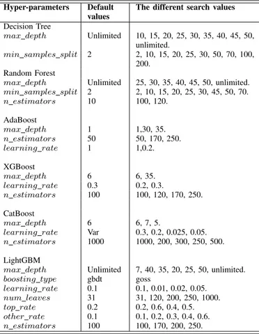
Finding relevant features and the choice of the right algo-rithm is not enough, we should also find the right configuration of the algorithm for a dataset by tuning its hyper-parameters (Figure 1), i.e., parameters that will not be learned from the training process [21]. For more details, Table I presents the default and the different hyper-parameters’ values explored for the tuning process of each classifier. The unmentioned hyper-parameters are set to default values.
V. RESULT ANALYSIS AND DISCUSSION
The first contribution of this paper is to find the optimum number of features that can provide the best classification in a real dataset. Then, we compare the efficiency of recently developed XGBoost, LightGBM, and CatBoost with other DT-based models include Decision Tree, AdaBoost, and Random Forest. Another contribution is that we study the impact of the default and tuned hyper-parameters on these classifiers. A. Feature selection of network traffic
As RF and DT are the simplest classifiers, we applied them to train and test the entire and the reduced dataset with feature selection methods. The obtained results are presented in Table II as well as in Table III. In the first step, we evaluated the classifiers with two features selection methods on different reduced versions of the data. We have tested feature subsets that contained 10, 15, and 25 features. Then, we test the accuracy and efficiency of the classification with the entire data against the best-selected features subsets (reduced dataset). According to Table II, we can see that DT and
1https://github.com/dmlc/xgboost. 2https://github.com/microsoft/LightGBM/tree/master/python-package. 3https://catboost.ai/docs/concepts/python-installation.html. 4 https://www.kaggle.com/jsrojas/ip-network-traffic-flows-labeled-with-87-apps TABLE I
DEFAULT AND THE POSSIBLE VALUES FOR EVERY HYPER-PARAMETERS IN THE DIFFERENT CLASSIFIERS
Hyper-parameters Default values
The different search values Decision Tree
max depth Unlimited 10, 15, 20, 25, 30, 35, 40, 45, 50, unlimited.
min samples split 2 2, 10, 15, 20, 25, 30, 50, 70, 100, 200.
Random Forest
max depth Unlimited 25, 30, 35, 40, 45, 50, unlimited. min samples split 2 2, 10, 15, 20, 25, 30, 45, 50, 70. n estimators 10 100, 120. AdaBoost max depth 1 1,30, 35. n estimators 50 50, 170, 250. learning rate 1 1,0.2. XGBoost max depth 6 6, 35. learning rate 0.3 0.2, 0.3. n estimators 100 100, 120, 170, 250. CatBoost max depth 6 6, 7, 5.
learning rate Var 0.3, 0.2, 0.025, 0.05. n estimators 1000 1000, 200, 300, 250, 500. LightGBM
max depth Unlimited 7, 40, 35, 20, 25, 50, unlimited. boosting type gbdt goss
learning rate 0.1 0.1, 0.01, 0.02, 0.05. num leaves 31 31, 120, 200, 250, 1000. top rate 0.2 0.2, 0.6, 0.4, 0.5. other rate 0.1 0.1, 0.2, 0.3, 0.4, 0.6. n estimators 100 100, 170, 200, 250.
RF models perform better with the 15-selected feature by RFE with 82.31% and 85.49% accuracy. Moreover, Table III indicates that these models can perform better with the reduced features set than with the entire dataset in term of accuracy, precision, and recall. A reason for these results is that not all features in our dataset will help to separate classes during the classification task.
TABLE II
CLASSIFICATION ACCURACY(%)WITHRFEANDIGON DIFFERENT FEATURES SET
Classifiers Top 10 Top 15 Top 25 IG RFE IG RFE IG RFE DT 81.38 80.18 81.93 82.31 81.58 82.19 RF 85.04 84.69 84.88 85.49 84.27 84.91
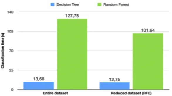
In order to illustrate the impact of feature selection on ML models, Figure 2 and Figure 3 present the training and test time with the entire and reduced (with features selected by RFE) dataset of DT and RF respectively. It can be seen that the feature selection method decreases the time required both for training and testing (by 72% for training and 6% for testing with DT; by 40% for training and 20% for testing
Fig. 2. Training time comparison Fig. 3. Classification time comparison
TABLE III
THE ACCURACY,PRECISION,AND RECALL(%)OF THE ENTIRE DATA AND
SELECTED DATA ANALYZED BYDTANDRF
Data size Accuracy Precision Recall Entire dataset + DT 82.16 81.94 82.16 Reduced dataset (RFE) + DT 82.31 82.13 82.31 Entire dataset + RF 82.52 83.13 82.50 Reduced dataset (RFE) + RF 85.49 85.82 85.49
with RF). Therefore, we can conclude that the classification performance is better on the reduced dataset as the models use less computation effort and still give more accurate results. It can be explained by the fact that this subset is more informa-tive to characterize our target classes (i.e. applications). For information, the 15 selected features are listed hereafter : Des-tinationIP, sourceIP, sourcePort, destinationPort, FlowIATMax, FwdI-ATTotal, Timestamp, FlowDuration, InitWinBytesBackward, InitWin-BytesForward, FwdPacketLengthMax, BwdPacketLengthMax, Sub-flowFwdBytes, BwdPacketLengthMean, FwdPacketLengthStd.
In the following, we will use the selected dataset with RFE as the input of the other classifiers, in consideration of more accurate classification of traffic as well as a greatly reduced training and classification time.
B. Performance analysis of traffic classification
Using the selected 15-features set identified in the feature selection process, a comparative analysis of six DT-based mod-els has been performed considering accuracy and computation time as the classifiers’ efficiency measurement.
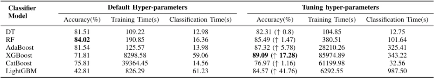
Table IV presents the accuracy of the different classifiers with default hyper-parameters against tuned hyper-parameters. The best accuracy among all classifiers was the accuracy of the XGBoost with tuned hyper-parameters model at 89.09%. Also, the difference between tuned and default settings of XGBoost, AdaBoost, and especially LightGBM is high while this is not the case for CatBoost because it performs an internal adjustment of the learning rate. Moreover, the difference between tuned and default hyper-parametrizations of RF and DT is small. Therefore, according to the results presented in this table, we can remark that the search for optimal hyper-parameters is necessary to create accurate models especially, for boosting-based models. Last but not least, the top-3
classifiers having the best accuracy belong to the ensemble methods namely XGBoost, Random Forest, and AdaBoost with 89.09%, 85.49%, and 84.57% accuracy.
Moreover, this table also illustrates the model building time (training time) and the classification time (testing time) using the default and tuned hyper-parameters. The main deficiency found in the experiments is the time cost for the training of the boosting algorithms and online classification. From this table, we can see how the tuned hyper-parameters increase the training and classification time for the ensemble learning and especially for the boosting algorithms. For instance, building the model (i.e., training time) of Adaboost, XGBoost, and LightGBM with default hyper-parameters performs respec-tively 225x, 10x, and 8x faster than they are with tuned hyper-parameters. Since this incurs significant computation cost and is therefore unsuitable especially for network traffic classification systems that require persistent training. Also, we must consider the time spent to find the optimal set of hyper-parameters for the boosting algorithms.
C. Concluding remarks
In order to summarize the results obtained, we can no-tice that XGBoost obtains the best results in generalization accuracy. LightGBM training is the fastest of all boosting algorithms and the slowest one for online classification. Tuned XGBoost and LightGBM perform generally better than their default versions. Moreover, despite AdaBoost one of the oldest boosting method, it provides competitive results. Also, DT accuracy ranges from 81.51% with its default-parameters to 82.31% with the tuned version. This indicates that the difference between the default settings of DT and the tuned version is small and hence it is not impacted by the hyper-parameters. Furthermore, boosting-based learning algorithms have limitations, such as the determination of the optimal hyper-parameters for achieving efficient predicted model. Another important aspect of the default version of RF provides competitive results (i.e., accuracy and speed) without the computational burden of hyper-parameters tuning and it is usually easier to apply than others. Finally, from the experiments of this study, the majority of classification techniques yielded classification performances that are quite
TABLE IV
CLASSIFICATION PERFORMANCE AND COMPUTATIONAL EFFICIENCY OF THE DIFFERENT MODELS(IN SECONDS)USING DEFAULTS AND TUNING HYPER-PARAMETERS SETTINGS
Classifier Model
Default Hyper-parameters Tuning hyper-parameters
Accuracy(%) Training Time(s) Classification Time(s) Accuracy(%) Training Time(s) Classification Time(s) DT 81.51 109.22 12.98 82.31 (↑ 0.8) 104.85 12.75 RF 84.02 190.85 16.36 85.49 (↑ 1.47) 380.51 101.64 AdaBoost 81.54 125.57 13.98 87.32 (↑ 5.78) 28210.26 325.41 XGBoost 71.81 8298.58 59.06 89.09 (↑ 17.28) 85974.89 343.22 CatBoost 75.81 39364.45 14.56 76.97 (↑ 1.16) 61199.98 32.56 LightGBM 42.81 826.29 61.23 84.57 (↑ 41.76) 6292.55 987.50
competitive with each other. It is hence left to the user to adopt an appropriate algorithm to their requirement and environment.
VI. CONCLUSION AND FUTURE WORK
In this paper, we have presented data analysis and explo-ration techniques to select the most relevant features that can be used for network traffic classification. Then, an empirical analysis of different DT-based traditional classifiers (DT, RF, AdaBoost) as well as the recently developed CatBoost, Light-GBM, and XGBoost classifiers, has been conducted. This com-parison has been carried out with the data subset selected via Recursive Features Elimination (RFE). Using RFE, we have derived a mechanism to identify the best 15 features out of 87 features in our dataset. This has not only significantly reduced the execution time but also has identified useful features for network traffic classification in a real-world dataset to increase the ML models’ accuracy. Furthermore, experimental results and analysis have shown that more features do not always improve the classification performance. Moreover, from the DT-based models’ comparison, we conclude that the hyper-parameter search is necessary to construct accurate boosting-based models where this is not the case for DT and especially RF that generalize well with the default hyper-parameters.
Our future work will focus more on the effect of each hyper-parameters on the performance (accuracy and speed) of the classifiers with more datasets. Also, another future direction that could be conducted, as a result of these findings, would be to consider a stacking approach for network traffic classification through the combination of multiple techniques.
REFERENCES
[1] M. I. Jordan and T. M. Mitchell, “Machine learning: Trends, perspec-tives, and prospects,” Science, vol. 349, pp. 255–260, 2015.
[2] A. Janecek, W. Gansterer, M. Demel, and G. Ecker, “On the relationship between feature selection and classification accuracy,” vol. 4, pp. 90– 105, 2008.
[3] C.-T. Chu, S. K. Kim, Y.-A. Lin, Y. Yu, G. Bradski, K. Olukotun, and A. Y. Ng, “Map-reduce for machine learning on multicore,” in Advances in neural information processing systems, pp. 281–288, 2007. [4] A. L’heureux, K. Grolinger, H. F. Elyamany, and M. A. Capretz,
“Machine learning with big data: Challenges and approaches,” IEEE Access, vol. 5, pp. 7776–7797, 2017.
[5] T. T. Nguyen and G. Armitage, “A survey of techniques for internet traffic classification using machine learning,” IEEE communications surveys & tutorials, vol. 10, pp. 56–76, 2008.
[6] S. Sen, O. Spatscheck, and D. Wang, “Accurate, scalable in-network identification of p2p traffic using application signatures,” in Proceedings of the 13th international conference on World Wide Web, (New York NY USA), pp. 512–521, May 2004.
[7] Z. A. Qazi, J. Lee, T. Jin, G. Bellala, M. Arndt, and G. Noubir, “Application-awareness in SDN,” in Proceedings of the ACM SIG-COMM conference on SIGSIG-COMM, (Hong Kong, China), pp. 487–488, August 2013.
[8] P. Perera, Y.-C. Tian, C. Fidge, and W. Kelly, “A comparison of super-vised machine learning algorithms for classification of communications network traffic,” in International Conference on Neural Information Processing, pp. 445–454, Springer, 2017.
[9] M. Shafiq, X. Yu, A. A. Laghari, L. Yao, N. K. Karn, and F. Abdessamia, “Network traffic classification techniques and comparative analysis using machine learning algorithms,” in 2016 2nd IEEE International Conference on Computer and Communications (ICCC), pp. 2451–2455, IEEE, 2016.
[10] O. Aouedi, K. Piamrat, and D. Bagadthey, “A semi-supervised stacked autoencoder approach for network traffic classification,” in Proceedings of the 28th International Conference on Network Protocols (ICNP), (Madrid, Spain), October 2020.
[11] M. P. J. Kuranage, K. Piamrat, and S. Hamma, “Network traffic classification using machine learning for software defined networks,” in Proceedings of the International Conference on Machine Learning for Networking, (Paris, France), pp. 28–39, December 2019.
[12] I. Guyon and A. Elisseeff, “An introduction to variable and feature selection,” Journal of machine learning research, vol. 3, pp. 1157–1182, 2003.
[13] G. Ke, Q. Meng, T. Finley, T. Wang, W. Chen, W. Ma, Q. Ye, and T.-Y. Liu, “Lightgbm: A highly efficient gradient boosting decision tree,” in Advances in neural information processing systems, pp. 3146–3154, 2017.
[14] J. Novakovic, “Using information gain attribute evaluation to classify sonar targets,” in Proceedings of the 17th Telecommunications forum, (Belgrade, Serbia), pp. 1351–1354, November 2009.
[15] F. Salo, A. B. Nassif, and A. Essex, “Dimensionality reduction with ig-pca and ensemble classifier for network intrusion detection,” Computer Networks, vol. 148, pp. 164–175, 2019.
[16] G. H. John, R. Kohavi, and K. Pfleger, “Irrelevant features and the subset selection problem,” in Machine Learning Proceedings 1994, pp. 121– 129, 1994.
[17] R. Polikar, “Ensemble based systems in decision making,” IEEE Circuits and systems magazine, vol. 6, no. 3, pp. 21–45, 2006.
[18] Y. Freund and R. E. Schapire, “A decision-theoretic generalization of on-line learning and an application to boosting,” Journal of computer and system sciences, vol. 55, pp. 119–139, 1997.
[19] T. Chen and C. Guestrin, “Xgboost: A scalable tree boosting system,” in Proceedings of the 22nd acm sigkdd international conference on knowledge discovery and data mining, pp. 785–794, 2016.
[20] A. V. Dorogush, V. Ershov, and A. Gulin, “Catboost: gradient boosting with categorical features support,” arXiv:1810.11363, 2018.
[21] A. Zappone, M. Di Renzo, and M. Debbah, “Wireless networks design in the era of deep learning: Model-based, ai-based, or both?,” IEEE Transactions on Communications, vol. 67, pp. 7331–7376, 2019.