To link to this article :DOI :10.
1063/1.4743026
URL : http://dx.doi.org/10.1063/1.4743026
To cite this version
Van der Geld, Cees and Colin, Catherine and Segers ,
Quint and Pereira da Rosa, V.H. and Yoshikawa, Harunori Forces on a
boiling bubble in a developing boundary layer, in microgravity with g-jitter
and in terrestrial conditions. (2012) Physics of Fluids, vol. 24 (n ° 082104).
ISSN 1070-6631
O
pen
A
rchive
T
OULOUSE
A
rchive
O
uverte (
OATAO
)
OATAO is an open access repository that collects the work of Toulouse researchers and
makes it freely available over the web where possible.
This is an author-deposited version published in :
http://oatao.univ-toulouse.fr/
Eprints ID : 9790
Any correspondance concerning this service should be sent to the repository
administrator:
[email protected]
Forces on a boiling bubble in a developing boundary layer,
in microgravity with
g
-jitter and in terrestrial conditions
C. W. M. van der Geld,1,a)C. Colin,2Q. I. E. Segers,1
V. H. Pereira da Rosa,1and H. N. Yoshikawa2
1Department of Mechanical Engineering, Eindhoven University of Technology, P.O. Box 513, 5600 MB Eindhoven, The Netherlands
2Inst. de M´ecanique des Fluides de Toulouse, UMR CNRS/INPT/UPS 5502, 2 Avenue Camille Soula, 31400 Toulouse, France
Terrestrial and microgravity flow boiling experiments were carried out with the same test rig, comprising a locally heated artificial cavity in the center of a channel near the frontal edge of an intrusive glass bubble generator. Bubble shapes were in micrograv-ity generally not far from those of truncated spheres, which permitted the computation of inertial lift and drag from potential flow theory for truncated spheres approximat-ing the actual shape. For these bubbles, inertial lift is counteracted by drag and both forces are of the same order of magnitude as g-jitter. A generalization of the Laplace equation is found which applies to a deforming bubble attached to a plane wall and yields the pressure difference between the hydrostatic pressures in the bubble and at the wall, 1p. A fully independent way to determine the overpressure 1p is given by a second Euler-Lagrange equation. Relative differences have been found to be about 5% for both terrestrial and microgravity bubbles. A way is found to determine the sum of the two counteracting major force contributions on a bubble in the direction normal to the wall from a single directly measurable quantity. Good agreement with expectation values for terrestrial bubbles was obtained with the difference in radii of curvature averaged over the liquid-vapor interface, h(1/R2 − 1/R1)i, multiplied
with the surface tension coefficient, σ . The new analysis methods of force compo-nents presented also permit the accounting for a surface tension gradient along the liquid-vapor interface. No such gradients were found for the present measurements.
I. INTRODUCTION
The general aim of much boiling research has been in the past, and still is today, the prediction of histories of bubble size and shape.1In particular, the bubble volume at detachment plays a role in much mechanistic modeling of boiling and prediction of heat flux.2 Knowledge of the forces acting on a bubble is not only essential to predict its trajectory; it may serve as a basis to build correlations for heat transfer1or mechanistic models3upon. Force expressions are required to infer accelerations from Newton’s second law of motion. The resulting second order differential equations for the position of the bubble are subsequently integrated and supplied with an appropriate set of initial positions and velocities in order to predict trajectories. Some of the forces involved result from the flow field of the fluid around the bubble. These so-called hydrodynamic forces can in principle be determined by solving local balances of mass and momentum in a numerical approach (CFD). The hydrodynamic forces are alternatively determined from empirical correlations which are usually expressions in terms of the local, instantaneous velocities of the bubble and the undisturbed flow field.4Axisymmetric bubble growth in pool boiling at a horizontal surface in an otherwise quiescent
liquid has successfully been predicted in the above Newtonian approach with analytical means with the neglect of inertia.5In this case, possible bubble shapes depend on the ratio of capillary to gravity forces. Detachment occurs in axisymmetric pool boiling if no possible shapes for a given bubble volume and a given foot radius exist.5Bubble detachment in pool boiling has also been investigated by direct numerical simulation.6
The present study is based on an alternative to the above-mentioned Newtonian treatment of bubble dynamics. It utilizes Euler-Lagrange equations which have proven to be a convenient approach if a bubble is deforming.7,4,8,9This Euler-Lagrange approach facilitates extension of the above-mentioned Newtonian approach to bubbles without axisymmetry and to bubbles with an axisymmetric shape in a uniform flow field. In this paper, the approach is used to analyze new bubble growth measurements performed in flow boiling on earth and in parabolic flights, with the same set-up in identical process conditions. The bubbles thus measured will be named terrestrial and microgravity bubbles, respectively.
Ways will be explored to determine the sum of two major force contributions in the direction normal to the wall directly from a single measured quantity, rather than from assessments of these forces individually. Terrestrial bubbles with more or less known growth characteristics will be used to examine solutions presented. Particular attention will be given to the determination of the pressure inside the bubble, the so-called overpressure. Two independent ways to determine the overpressure will result from the Euler-Lagrange analysis in a natural way and results will be compared for both terrestrial and microgravity bubbles. In the literature, sometimes the Laplace equation is used to assess the overpressure.10,11 The present paper will present another expression, based on the first Euler-Lagrange equation for the isotropic component of the contour, which is valid for deformed bubbles. To satisfy a balance of estimated force components normal to the wall, a correction parameter is often used to multiply the overpressure with.12,13The present analysis will be shown to be accurate enough not to need such a correction parameter and is useful for the development of point force models.
As for differences with our previous publications, the new analyzing method may appear to be a straightforward extension of the analysis of previous publications, but it is not. The bubbles studied in Ref.8were deforming in the proximity of a plane wall but were without a bubble foot at the wall. In Refs.10and11, the bubble was attached to the wall, but it was assumed to have a spherical shape. The bubbles studied in Refs.7and9had exactly the shape of truncated spheres while those of the present study do not. In Ref.7, only one governing equation was considered and in the present study more. In Refs.7 and9, the overpressure force exactly balances the capillary force, which means that the sum of these two dominant forces vanishes identically to zero. This is obviously impossible for terrestrial bubbles in the experiments of the present study and the new analysis is therefore for arbitrary bubble shape of a bubble with a foot at a plane wall. Buoyancy will be shown to be balanced by the sum of the two dominant forces and only slight deformation of the bubble is necessary to resettle this balance during bubble growth.
II. EXPERIMENTAL
The experimental test rig was developed at Institut de M´ecanique des Fluides de Toulouse (IMFT) in France and the test section and bubble generator used for the experiments described in this paper at Eindhoven University of Technology (TU/e). The experiments were conducted by IMFT, with people of TU/e participating by invitation, during the 50th Parabolic Flight Campaign of May 2009 at Novespace, Bordeaux in France. The same setup was used for terrestrial experiments at IMFT. Microgravity during the elliptic top part of the airplane trajectory lasted for 21 sec.
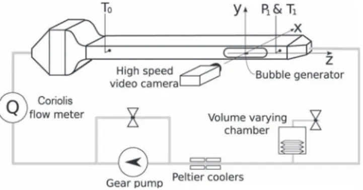
The loop (Fig.1) comprises a straight inlet section of 360 mm with a diverging and converging test section and a honeycomb in between. The inlet section is followed by a straight channel of 600 mm to make the flow fully developed in the test section (170 mm length) positioned downstream. Internally, the rectangular channels measures 5 × 40 mm2. A constant pressure volume compensator
is used to keep the system pressure constant with the aid of an air volume behind a membrane. Fluid is HFE7000 that boils at 34◦C at 1 bar. System pressure was set at 1.1 bar corresponding to
FIG. 1. Schematic of test rig.
a saturation temperature of 37◦C. Inlet subcooling was 4◦C, so inlet temperature of the liquid was
33◦C. Fluid was degassed for 5 h before having it filling the test loop which was made vacuum.
Test section is made of stainless steel with the aid of electric discharge machining. A glass bubble generator is positioned in the center of the test section such that an artificial cavity, with a volume of about 1 mm3, ends in an elliptical mouth in the very center of the channel (Fig.2). The major axis of the ellipse was in flow direction and measured 0.17 mm, while the shortest axis measured 0.033 mm; area of the cavity mouth is 0.018 mm2. This cavity mouth is positioned at a distance of 0.493 mm of the sharp edge of the bubble generator (Fig.2).
Thin films are sputtered with microwaves onto the glass to get an area of about 1 × 1 mm2(0.947
× 0.789 mm2to be precise) around the cavity mouth covered by a titanium coating, with a typical thickness of 500 nm. Bubble radius is less than 1 mm so heat flux from the thin film to the bubble is not hampered by size limitations of the heating area. The titanium coating has a good adherence to the glass. The two leads towards the heated bubble generation site are made of titanium with a gold layer on top, see Fig.2where the gold is shown as a lighter grey on line. Electric resistance is only high at the heating area of 1 × 1 mm2. The leads are connected to a power supply.
The flow approaching the sharp edge of the glass bubble generator is as uniform as it can be in the channel used. Downstream of the sharp edge a boundary layer starts developing. Two
FIG. 2. View from above onto the flat surface on which bubbles are created. The irregular rim in the top of this picture is the edge of the coated glass bubble generator and below this edge the bubble generator is seen, with uncoated glass in black and with golden leads (shown lighter grey on line) coming from left and right towards the dark square around the artificial cavity. Heat is generated uniformly in the coating of the latter square (darker grey, bluish on line). The black bar on the top left of the figure is a scale that measures 1 mm. Flow direction is from top to bottom, normal to the frontal edge. The artificial cavity ends as an ellipsoidal hole with axis 0.17 mm and 0.033 mm.
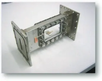
FIG. 3. Photograph of the bubble generator mounted in the stainless steel test section. The slit on the left is the outlet and measures 40 × 5 mm2.
polycarbonate (LexanTM, fabricated by SABIC Innovative Plastics, The Netherlands) windows
permit visual observations from the side (Fig.3). Estimates, to be discussed in Sec. IV A, show that while bubble nucleation occurs inside the boundary layer, most of the liquid-vapor interface is outside it during bubble growth until the bubble detaches and moves downstream, see Fig.4.
Bulk liquid flow rate is measured with a Coriolis flow meter, type Micromotion R025S (Fig.1). The measurements presented in this paper were performed with a liquid velocity that amounted to 0.0120 ± 0.0004 m/s at the location of the bubble generator, with a profile that fairly constant at the scale of bubble diameters measured. This profile was characterized by a series of PIV measurements. The flow can be laminar or turbulent depending of the bulk Reynolds number. For the results presented hereafter, it is a laminar fluid flow, with a bulk Reynolds number of about 300 based on a kinematic viscosity of 3.2 × 10⁻⁷ m2/s, a volume flow rate of 2.14 × 10⁻⁶ m3/s, channel widths 5 and 40 mm. Accelerometers, to measure g-jitter (typically 0.045 m/s2), temperature and pressure sensors were recorded at 2 kHz and video-recordings of bubble growth were made at 500 Hz. Diffuse background illumination with a halogen lamp was applied and each image was after cropping, to save storage capacity, composed of 1280 × 700 pixels. Size calibration was done both with a scale with equidistant lines of 0.1 mm and by moving the camera with the aid of a micrometer
FIG. 4. Bubble growing in a boundary layer in microgravity; approaching liquid velocity V = 1.2 cm/s, coming from the left. Diameter of the bubble on the LHS is 0.2 mm. Asymmetry between front and rear of this small bubble is barely observed. The large bubble on the RHS is fully detached from the wall directly after its creation by coalescence of two smaller bubbles. In the corresponding movie, the bubble is observed to grow and slide downstream, to the RHS of the figure.
screw gauge. Conversion factor is 0.00198 mm/pixel with an uncertainty of 2%. Each photograph of a video-recording is separately analyzed, in a way described in Sec.III A.
III. FORCE ANALYSES
A. Determination of generalized coordinates
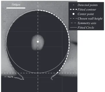
Each 2D-image of a bubble is in grayscale and inverted in grayscale to facilitate the subtraction of a reference figure without a bubble but with the physical wall. The latter reference figure not always exists if the solid wall is moving in the camera view (microgravity experiments). The resulting image is cropped and rotated before a median filter is applied once and a Gaussian filter applied three times in order to remove inaccuracies due to pixel resolution limitations. Then the zero-cross method is used to determine points on the liquid-gas interface. These points are subsequently connected in an edge-line determination procedure.
Since the fluid flow parallel to the wall might have caused asymmetry in the projected shape of the bubble, the smoothed bubble contour is split into two halves in the following way. First, a chosen wall is selected parallel to the actual, solid wall on which the bubble is attached, see Fig.5. The chosen wall could be on top of the actual wall but is usually selected to be positioned in the fluid region at a small distance from the actual wall. This is possible since the force balances that will be derived need to be satisfied for arbitrary bubble volume bounded by part of the measured contour and a chosen wall. Only the estimates of the hydrodynamic forces to be presented decrease in accuracy with increasing distance of the chosen wall to the actual wall. This, however, will be seen to have hardly any consequence for the conclusions that will be drawn. The cross-section of the bubble contour with the chosen wall is a line. Let the length of this line be 2rfoot, which defines rfoot.
Next, the top of the bubble is determined as the point furthest away from the chosen wall. Suppose that ˆy is a unit vector of a Cartesian coordinate system in the projection plane pointing towards the chosen wall and normal to this wall. If the chosen wall has coordinate ywalland the top of the bubble
has coordinate ytopthen the maximum height of the bubble is given by ywall– ytop. The line through
the top of the bubble normal to the actual wall is the line on which the center of the bubble, O, will be found and is also the line that splits the bubble in two halves. The right hand side of the bubble by definition is the half which is downstream of the fluid flow. This right hand side is mirrored to the line through the top and O in order to obtain a fully symmetrical bubble contour. The bubble is assumed
Detected points Fitted contour Center point Chosen wall height Symmetry axis Fitted Circle 100µm
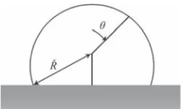
FIG. 6. Polar coordinate system with radial distance of the center to the bubble foot, ˇR.
to be axisymmetric around the line through the top and O and the applicability of this assumption is assessed in the following way. The cross-section of the present contour with the chosen wall has a length, which is compared with 2rfoot. Differences turn out to be about 2%, which is considered
as acceptable in view of the difficulty to measure the bubble foot and the similarity to a sphere of the top of the bubble (Fig.5). This similarity is quantified in the next paragraph. The length rfoot is
retained in the following in order to increase accuracy of the determination of the area of the bubble in contact with the chosen wall.
The center of the bubble is determined as follows. A circle with radius Rsphereis fitted through
contour points near the top of the bubble. When gravity is terrestrial, the shape of the bubble is such that the radius of curvature of the bubble is continuously varying near the top and depends on coordinate y. Because of this there is some arbitrariness in the determination of Rsphere. However,
the present analysis is aimed at a comparison of measured contours with those of truncated spheres and a value of a circle radius is therefore needed which makes the arbitrariness unavoidable. It is obvious that the fewer contour points are used to determine Rsphere, the closer its value will be to one
of the radii of curvature at the bubble top and the more unique the value of Rsphere. For comparison
with the truncated sphere shape it is better to select more points at the contour. The determination of
Rsphereis done by least square fitting of a circle through the selected contour points. Figure5shows a typical result.
In the analysis of histories of boiling bubbles shaped as truncated spheres it is customary to use (h, Rsphere) as the coordinates of the bubble. For this reason, distance h of the center O from
the chosen wall is considered a generalized coordinate in the present analysis. Inertia and drag forces will be estimated using only h and Rsphere as coordinates, but only because no expressions
are available for inertia and drag that take further deformation into account. If gravity is terrestrial and/or governing Reynolds numbers are big, however, deformation cannot be neglected. In our experiments at microgravity, typical value of the Weber number, We = ρLV2 2Rsphere/σ, is 0.002
(V = 0.012 m/s, Rsphere = 0.15 mm, ρL is mass density of the liquid, and σ is surface tension
coefficient), which proves that the bubble deformation is negligible in this case. Governing Reynolds numbers are based on length scale Rsphere and velocity scales ˙Rspher e= dRsphere/dt or U, the time
rate of change of h, or V, the approach velocity parallel to the wall of the fluid at the center O, which is taken to be a uniform approach velocity; t denotes time. Since deformation cannot always be neglected, Legendre coefficients are determined as generalized coordinates further to h as follows.
Define x = cos(θ) with θ the polar angle measured from the top of the bubble in the polar coordinate system centered at center O, see Fig.6. Let θ1 be the angle corresponding to the foot
of the bubble at the chosen wall, corresponding to radial distance ˇRof this foot, such that cos(θ1)
= – h/ ˇR. Only if for all θ radial distance R(cos(θ)) of the contour equals Rspherethe shape is that of
a truncated sphere with radius ˇR = Rsphereand height h above the chosen wall.
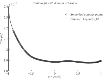
Let the holonomic constraint r = R(cos(θ), t) represent the measured contour on [cos(θ1), 1]. This constraint is applicable to all measured shapes. The extension R¸ of R is defined by
R¸ (x) = R(x) if x ≥ cos(θ1) and if x < cos(θ1) then
−1 −0.5 0 0.5 1 1.8 1.9 2 2.1 2.2 2.3 2.4x 10 −4 x = cos(θ) R(x) [m]
Contour fit with domain extension
Smoothed contour points Fourier−Legendre fit
FIG. 7. Typical example of measured contour points (“Data points”) with second order extension to improve accuracy of curvature determination at the bubble foot (x = –0.85) and Legendre fit (solid line).
with constants d1and d2such that the curvature at cos(θ1) can accurately be evaluated. This requires
a smooth, twice differentiable continuation at cos(θ1). Let Lej–1denote the Legendre polynomial of
order j–1 (Le0= 1). Fourier-Legendre coefficients of R¸, bj, are defined by
R¸ = 6jb˜jLej −1(cos(θ )) = 6jb˜jLej −1(x), (1)
and the ˜bj are determined by integration in the usual way. Indices in the summation run from 1 to
25. For sake of brevity, » is defined by
»= cos(θ1). Let
a1= ∂ R/∂x|»and a2=1/2/2 ∂2R/∂ x2|».
The smooth continuation obviously requires that d1 = a1 and d2 = a2. Figure7 shows a typical
example of an extended bubble contour R(x).
It turns out with properly selected distance h, ˜b2is much less than both ˜b1and h. The absolute
value of the ratio of ∂ ˜b2
∂t to
∂h
∂t = ˙h = U is less than 2% in all measurements. Since for a free bubble hand ˜b2are dependent, the following parameters are selected as generalized coordinates: b1= ˜b1,
b2 = h, b3 = ˜b3, b4 = ˜b4, b5 = ˜b5, etc. The value of b1, or ˜b1, can be seen as the mean distance
of the bubble contour to the center point. The value of b1is close to that of Rsphere if the bubble is
nearly a truncated sphere. In integrals and other expressions involving contour fit R(x) or R¸ (x), all ˜
bj-coefficients are taken into account. In one case this yields a correction coefficient c1= 1 +˙˜b2/U
in an integral.
Two brackets will be used to indicate an average over the entire gas-liquid interface. For example, the average hRi is given by
hRi = Z 1 » d x R(x)/(1 − ») = { Z θ1 0 dθ R(θ ) sin(θ )}/(1 − cos(θ1)).
B. Determination of the main force components
When the generalized coordinates defined in Sec.III Aare used, Newton’s law of motion has to be transformed and expressions for the corresponding generalized forces have to be derived. This has been done in a derivation that starts from the so-called mechanical energy balance for the fluid surrounding the bubble.9The resulting time rate of change of the kinetic energy, T, can be given the
form
d T
dt = 1p dVb/dt + σ d Ab/dt + ...,
where the dots indicate expressions whose components are specified below. Volume and area of the bubble are Vband Ab, respectively, while σ is the surface tension coefficient and 1p the pressure
difference between the homogeneous pressure inside the bubble and the pressure in the liquid near the solid wall on which the bubble is footed. There is no restriction on kinetic energy T in this stage; it accounts for turbulence as well as for creeping flow. The RHS of this equation can be written as the sum of products of generalized forces, Fj, and generalized velocities, qj= ˙bj: dT/dt =Pj Fj qj. It is now assumed that the fluid flow is solenoidal which is, for example, satisfied if the fluid is incompressible. The LHS of the above equation can then be written as the sum of the time rates of change of a purely irrotational component, Tirrot, of a purely vector potential component, Tvort, and
of a mixed component, Tmixed. This is because the velocity field is the sum of an irrotational scalar
component and a solenoidal vector potential component.14 The component Tirrotcan be expressed
in terms of added mass coefficients. In the general case, when the vorticity contribution cannot be neglected, equations of the following form are derived (j runs from 1 to 25):
− Fji ner ti a− F vor t j = F 1p j + F σ j + F g j + F dr ag j , (2)
where force Fjvortaccounts for the purely vector potential and mixed components. On the RHS of
Eq.(2), each Fjrepresents a generalized force which will be defined below and which corresponds
to generalized coordinate bj. It is noted that the forces which are here denoted as inertia forces, Fjinertia, stem from Tirrotand retain their form whatever the values of Tvortand Tmixed. The reason for
this is that the added mass forces and added mass coefficients stay the same in viscous flows.4,15A uniform approaching flow with velocity V parallel to the wall yields a potential flow lift contribution to the force balance in the direction perpendicular to the solid wall (labeled with “2”), which is in
F2inertia. Lift contributions to this force balance, which are related to vorticity are accounted for by
F2vort. Lift and other hydrodynamic forces are further discussed below.
The gravitational forces, Fjg, as well as the surface tension forces, Fjσ, turn out to be expressible
as integrals over the gas-liquid interface. The surface integrals mostly can be expressed in quantities prevailing at the bubble foot, the part of the bubble in contact with the solid wall. These quantities are mostly familiar ones. However, the measurement accuracy of these quantities is usually not high because of the so-called mirage effect16and since the wall is not measured as a sharp line (Fig.5). This is important for the analysis of forces based on measured shapes of a bubble attached to a wall. The present study will compare quantities measured at the bubble foot with values determined from corresponding surface integrals.
Equation(2) is valid for j = 1 to 25, which implies that 25 governing equations exist. The present analysis focuses on the isotropic component b1 and translational motion described by
b2= h because of the wish to compare with truncated sphere bubbles described by the two length
scales Rsphereand h. This means that the system of equations given by(2)is reduced to two equations
in 25 generalized coordinates and 25 generalized velocities which can be given the following form: −F1i ner ti a(bj, ˙bj, ¨bj) = F1vor t(bj, ˙bj) + F 1p 1 (bj) + F1σ(bj) + F g 1(bj) + F dr ag 1 (bj, ˙bj), −F2i ner ti a(bj, ˙bj, ¨bj) = F2vor t(bj, ˙bj) + F 1p 2 (bj) + F2σ(bj) + F g 2(bj) + F dr ag 2 (bj, ˙bj).
Here, the occurrence of (bj, ˙bj, ¨bj) indicates dependency on all generalized coordinates, generalized
velocities, and generalized accelerations; ¨h denotes the second order derivative of h with respect to time. As the inertia force will be seen to be linear in the generalized velocities, the above are two coupled second order differential equations in the generalized coordinates. Despite the fact that
Fj1p, F
jσ, and Fjg(j = 1,2) are only dependent on the generalized coordinates, i.e., on the shape of
the bubble, they are the dominant forces that must be determined from experimental observations with a high accuracy. This determination is the subject of the remainder of this section.
The first force on the RHS of(2)is F1p, the force due to the overpressure inside the bubble. The
overpressure is defined by 1p = (pb– pw), pbbeing the homogeneous pressure inside the bubble
and pwbeing the hydrostatic pressure in the fluid at the actual, solid plane wall. The overpressure
force components, Fj1p, follow from
F1j p= 1p ∂Vb/∂bj, (3)
where Vbdenotes the volume of the bubble. In expression(3)the overpressure 1p is an unknown
which occurs in each governing equation, labeled by j, of(2). The overpressure inside the bubble is related to heat transfer and since the energy equation is not solved for the experimental conditions at hand it is a time-dependent quantity, which must be determined from measurement data. Hydro-dynamic stresses near a bubble can be estimated as 1/2 ρL R˙spher e2 which is typically about 0.07 Pa
for a microgravity bubble and 0.002 Pa for a terrestrial bubble. If hydrodynamic stresses near the bubble foot at a chosen wall (see Sec.II) can be neglected, the so-called dynamic stress boundary condition across the liquid-gas interface at the bubble foot gives the following expression for the overpressure 1p:
1p = −2σ H |foot− ρLg hwall, (4)
where H|footis the negative mean curvature at the bubble foot and hwallis the height of the chosen
wall above the actual wall. An expression of the mean radius of curvature will be given below. A typical value of –2σ H|footis 200 Pa and of ρLg hwallis 0.1 Pa, which shows that the latter, hydrostatic
term is only a minor correction. Moreover, the above estimates of hydrodynamic stresses are even less, and therefore negligible indeed. In the present study, the overpressure will be determined in various ways in an attempt to increase the accuracy of the measurement result. Ways other than with
(4)to determine the overpressure are described below.
The partial derivatives ∂Vb / ∂bj in(3)are for j = 1 and j = 2 readily determined from the
measured shapes with the aid of the following measurable quantities: hR2i = Z 1 » d x R2(x)/(1 − ») = { Z θ1 0
dθ R2(θ )sin(θ )}/(1 − cos(θ1)), (5a)
hR3i = Z 1
»
d x R3(x)/(1 − »). (5b)
Note that » = cos(θ1) = – h/ ˇR. The first quantity, hR2i, is used to assess ∂Vb/ ∂b1from
∂Vb/∂b1= 2π(1 − »)hR2i. (6)
For a truncated sphere, ∂Vb/ ∂ b1= 2π ˇR( ˇR+h), with ˇR = Rshpere, since then hR2i = ˇR2. The volume
of the bubble follows from
Vb=2/3π(1 − »)hR3i +1/3πh( ˇR2− h2). (7)
It can be shown that
F2g = g ρ L Vb
with ρLbeing the mass density of the liquid. The other partial derivative of the bubble volume, for j = 2 in(3), is given by
∂Vb/∂b2=∂Vb/∂h=1/3π ˇR 2
− π h2= π r2f oot (8)
with rfoot, in principle equal to ˇRsin(θ1), evaluated as half the width of the chosen wall line crossing
The following definition is convenient in the force analysis below and represents the average of twice the mean curvature, 2H, over the entire gas-liquid interface:
h2H i = Z θ1 0 dθ R2(θ ) sin(θ ) 2H Á Z θ1 0 dθ R2(θ )sin(θ ), (9) where Rθ1 0 dθ R 2(θ ) sin(θ ) is equal to R1 » dx R 2 (x) = (1 – ») hR2
i. The mean radius of curvature is denoted with H and is given17as
((1))−1/2[1/2(R′/R)ctg(θ ) − 1 +1/2(R R′′− R′2)/((1))],
where ((1)) = R2 + R′2with R′ = ∂R / ∂θ, by definition and R′′ by definition the second order derivative of R with respect to θ . For a truncated sphere, H = –1/ ˇR = –1/Rshpere. The generalized
force Fσ2corresponding to h is given by
F2σ = 2πσ Z 1 » d x2H R (c1x R + p (1 − x2)R′)
with c1= (1 + ˙˜b2/U) a correction to velocity U for the bubble motion as a whole; note that on the
relevant domain of the polar angle, sin(θ ) =√(1 – x2). The ratio of time derivative ˙˜b2to U is usually
less than 0.02 for terrestrial bubbles and about –0.02 for the microgravity bubbles we measured. These values make c1effectively equal to 1. Taking c1= 1, the force Fσ2is given by
2π σ Z 1 » d x((1))−1/2 × [x{R′2− 2R2+ R((0))/((1))} + {R′((0))/((1)) − 2 R R′}p(1 − x2) + R R′x2/p (1 − x2)] (10) with ((0)) = (R2R′′– R R′2). It can be proven that this expression reduces to
− 2πrf ootσ sin(θc) (11)
with θcthe contact angle at the bubble foot measured in the liquid. The minus sign indicates action
into the direction opposite to h, so a force attracting the bubble towards the wall. The generalized force Fσ1corresponding to the isotropic component b1is given by
F1σ= 2πσ
Z 1
»
d x((1))−1/2[R R′x/p(1 − x2) − 2R2
+R((0))/((1))]. (12)
It can be proven that this expression reduces to
σh2H i∂Vb/∂b1. (13)
This expression reduces to −4πσ ( ˇR +h) for the case of a truncated sphere, with ˇR = Rshpere, since
h2Hi = –2/ ˇR then. The definition hx R3i = Z 1 » d x x R3(x)/(1 − ») (14)
makes it possible to express the gravity force F1gas follows:
F1g= g ρL2π (1 − ») (hhR2i + hx R3i). (15)
For a truncated sphere,(15)yields g ρLπ ˇR(h+ ˇR)2, with ˇR = Rshpere.
Collecting(3)and(13)into(2), we obtain for the isotropic component the following equation
(16)that can be considered as an extended Rayleigh-Plesset equation for a bubble attached to a plane wall. Expression(6)can be used to assess ∂Vb/ ∂ b1and(12)for F1g,
− F1i ner ti a− F vor t 1 = 1p ∂Vb/∂b1+ σ h2H i ∂Vb/∂b1+ F g 1 + F dr ag 1 . (16)
The drag force F1drag will be specified in Sec. III C below. A good approximation for the
overpressure is seen to be given by –σ h2Hi, since other contributions in(16)are usually less than this capillary term. This approximation is 2σ / ˇRin the case of a truncated sphere. A more accurate way to assess the overpressure 1p is easily obtained by rewriting(16),
1p = −σ h2H i − (F1i ner ti a+ F
g
1 + F
dr ag
1 )/(∂ Vb/∂b1).
The difference (–2σ H|foot+ σ h2Hi) is given by the (F1inertia+ F1g+ F1drag)-term on the RHS of
this equation.
Similarly, Eq.(17)for the second generalized coordinate, the distance of the center, h, to the wall, is obtained from(8),
− F2i ner ti a− F vor t
2 = 1p πr
2
f oot− 2πrf ootσsin(θc) + g ρLVb+ F2dr ag. (17)
Capillary force Fσ
2 is for (17) determined with(11), but Eq. (10) yields more accurate values,
usually. It can be proven that at the chosen wall
2H|f oot = 1/R1− sin(θc)/rf oot,
with R1a radius of curvature at the bubble foot while 1/R2 = –sin(θc) / rfoot is the other radius of
curvature. As a result, the neglect of hydrodynamic stresses near the bubble foot, leading to(4), yields
− F2i ner ti a− F vor t
2 = πr 2
f oot{ σ (1/R2− 1/R1)|foot− ρLg hwall} + g ρLVb+ F dr ag
2 . (18)
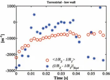
This remarkable result shows that the sum of the two major force contributions, the overpressure force and the capillary force, is a directly measurable quantity. The difference of the radii of curvature at the bubble foot is equal to the square root of 4H2 – K, where K is the Gaussian curvature. The difference can conveniently be determined from the measured contour and from
1/R2− 1/R1= ((1))−1/2R−1{R′ctg(θ ) − ((0))/((1))}. (19)
Although the gravity term – ρLg hwallin(18)is usually less than 1% of the capillary term it accounts
for much of the deformation of the interface, as can be observed by placing the chosen wall at various heights above the actual wall. The local values at the bubble foot in(18)are usually difficult to be measured accurately. For this reason another expression for F21p+ F2σis now given.
Let the mean difference between the inverses of the radii of curvature be defined by h1/R2− 1/R1i = Z θ1 0 dθ R2(θ ) sin(θ )(1/R2− 1/R1) Á Z θ1 0 dθ R2(θ ) sin(θ ). (20)
As long as 1p = –σ h2Hi is a sufficient approximation of the pressure difference between the bubble and the liquid at the chosen wall, the sum of the two major force contributions can be obtained from
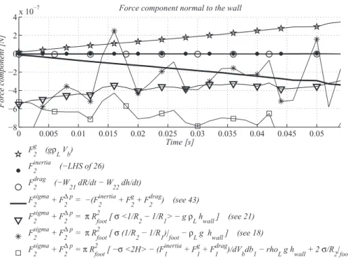
F21p+ F2σ = πr2f oot{σ h1/R2− 1/R1i − ρLg hwall}. (21)
Because of the averaging over the gas-liquid interface above the chosen wall,(21)is expected to give more accurate results from measured bubble contours than the formally more accurate following expression:
F21p+ F2σ = πr2f oot{−σ h2H i − (F1i ner ti a+ F1g+ F1dr ag)/(∂ Vb/∂b1) − ρLg hwall+ 2σ/R2|foot}.
(22) Here, averaging h2Hi is above the chosen wall and the radius of curvature 1/R2|footcan be determined
from –sin(θc)/rfootor from
1/R2= −((1))−1/2{1 − R−1R′ctg(θ )}. (23)
One of the main aims of the present study is to increase the measurement accuracy of force determinations. For this reason, the sum of the dominant forces F21p+ F2σ is assessed with the
aid of(18),(21)and(22)and compared with “ideal” values (1p2πrfoot2+ Fσ2), where 1p2is the
C. Hydrodynamic forces including drag
The remaining force components of Eq.(2) that need to be quantified are Fjinertia, Fjvort, and Fjdrag. The inertia forces are given by the Lagrange equation
d dt ∂Tirr ot ∂ ˙bj −∂T irr ot ∂bj = −F i ner ti a j .
The hydrodynamic force Finertiais computed from potential flow over truncated spheres. Up to this point in the analysis, general deformation of an axisymmetric bubble has been considered although the analysis was limited to the force balances corresponding to the first two generalized coordinated,
b1 and h. Since all three force components, Fjinertia, Fjvort, and Fjdrag, will be seen to have small
contributions and since the experimentally observed shapes of bubbles are close to that of truncated spheres, inertia, and drag forces will only be determined for that of the truncated sphere closest to the actual shape. This means that the governing equations are given by
−F1i ner ti a(b1, ˙b1, ¨b1,b2, ˙b2, ¨b2) = F1vor t(b1,b1,b2,b2) + F 1p 1 + F1σ+ F g 1 + F dr ag 1 (b1,b1,b2,b2), −F2i ner ti a(b2, ˙b2, ¨b2,b2, ˙b2, ¨b2) = F2vor t(b1,b1,b2,b2) + F 1p 2 + F2σ+ F g 2 + F dr ag 2 (b1,b1,b2,b2),
where the forces F1p, Fσ, amd Fg depend on all 25 generalized coordinates and are determined in
ways presented in the above Sec.III B.
A bubble with the shape of a truncated sphere (distance h and radius R) in a uniform flow field with velocity V experiences a lift force resulting from the induced pressure field. This lift force is part of F2inertia. To determine the inertia forces and viscous potential drag, the kinetic energy is
written as a second order polynomial of the two prevailing generalized velocities
Tirr ot/(1/2ρLV0) = αU2+ υ ˙R2
spher e+ ψ ˙Rspher eU + α2V2. (24)
Here, V0= 43πRsphere3. Each coefficient occurring on the RHS of this expression is an added mass
coefficient; coefficient υ was written as tr(β) in Ref.4. Each coefficient depends on generalized coordinates but not on generalized velocities. The coefficient α is familiar and has the value 0.5 far away from the wall. Values of added mass coefficients have been obtained both for spheres and truncated spheres.7,4In the present study, these added mass coefficients yield an estimate of Finertia by using Rsphere and h as parameters that characterize the truncated sphere with a shape closest to
the actually measured bubble shape. Convenient expressions to evaluate the added mass coefficients are given in the Appendix.
Viscous drag forces for truncated spheres can be determined from the potential flow field by the Levich approach.18,4Similar to the above determination of Finertia, drag force Fdragis overestimated
with the aid of measured parameters Rsphereand h that characterize the truncated sphere shape closest
to the actual bubble. The accuracy of the inertial lift and viscous potential drag will be discussed below. In the following equations, parameter Rsphere is written as R for sake of brevity and U is
written as ˙h to highlight similarity in the equations with respect to ˙R and ˙h. The Euler-Lagrange equation for the first generalized coordinate, Rsphere, yields
4 3π ρL R 3 0(1/2ψ ¨h + υ ¨R + M1) = F1vor t+ F 1p 1 + F σ 1 + F g 1 − W11R − W˙ 12h˙ (25)
(R0= R(t = 0), the initial value of b1) with inertia lift given by
M1= 1 2R˙ 2µ ∂υ ∂R + 3υ/R ¶ −1 2h˙ 2µ ∂α ∂R − ∂ψ ∂h + 3α/R ¶ + ˙h ˙R∂υ ∂h + 1 2V 2µ ∂α2 ∂R + 3α2/R ¶ . The Euler-Lagrange equation for h renders the second governing equation to the form
4 3π ρLR 3 0(α ¨h +1/2ψ ¨R + M2) = F2vor t+ F 1p E + F σ 2 + Vbg ρL− W21R − W˙ 22h,˙ (26)
with inertia lift given by
M2 = 1 2R˙ 2µ ∂ψ ∂R − ∂υ ∂h + 3ψ/R ¶ +1 2h˙ 2∂α ∂h + ˙h ˙R µ ∂α ∂R + 3α/R ¶ −1 2V 2∂α2 ∂h . (27)
Coefficients Wijare drag coefficients which only depend on the generalized coordinates (R = Rsphere
and h). For a sphere far away from the wall, both W11and W22reduce4,7 to 12π µ Rsphere. In Ref. 7, it was shown that literature results for the added masses for a touching sphere (λ = 12) and for
either ˙R = 0 or ˙R = U are in agreement with those obtained with the above approach. Convenient
expressions to evaluate W11and W22for a truncated sphere at a plane wall are given in the Appendix.
In the measurements of this study, bubble shapes are found to be close to those of truncated spheres. The range of applicability and the accuracy of the inertial lift and viscous potential drag for the measurements of this study will be discussed in Sec.III Ebelow.
D. Dimensionless form of the governing equations
The governing equations can be written in dimensionless form by dividing the dimensional equations by ρLR02R˙20, where ˙R0 is defined as the time rate of change of b1 at initial time zero,
˙
b1(t = 0), ˙h0is that of h at time zero, and R0is the initial value of b1. In boiling, ˙R0is bound to
be nonzero and positive which makes it a good reference velocity. The velocities ˙hand ˙R = ˙b1are
coupled by the governing equations, but velocity of the approaching flow at the center of the bubble,
V, is an independent velocity. Three Reynolds numbers exist:
Re1= ˙R0R0ρL/µ, Re2= ˙h0R0ρL/µ, ReV = V R0ρL/µ. (28)
Other dimensionless numbers are the Weber, Froude and dimensionless pressure numbers which are, respectively, defined by
W e = ρLR0R˙02/σ, Fr = ˙R 2
0/(g R0), 1P0= 1P(t = 0)/(ρLR˙20). (29)
With Wij= ˆWijb1π µ, the dimensionless governing equation corresponding to h becomes
4 3π R0((Re2/Re1) 2α ¨h/ h2 0+1/2ψ ¨R/ ˙R20) = − 4 3π ⌣ M2+ ⌣ F vor t 2 + π(r 2 f oot/R 2 0)1P0− 2π sin(θc)(rf oot/R0)/ W e + 4 3π(Vb/V0)/Fr − ˆW22π(b1/R0)( ˙h/ ˙h0)(Re2/Re1)/Re1− ˆ W21π(b1/R0)( ˙b1/ ˙R0)/Re1 (30)
with the inertia forces given by ⌣ M2 =1/2(R0 ∂ψ ∂b1 − R 0 ∂υ ∂h + 3ψ R0/R)( ˙b1/ ˙R0) 2 +1/2(Re 2/Re1)2( ˙h/ ˙h0)2R0 ∂α ∂h + (Re2/Re1) ( ˙h/ ˙h0)( ˙b1/ ˙R0)(R0 ∂α ∂b1 + 3α R 0/R) −1/2R0 ∂α2 ∂h (ReV/Re1) 2. (31) Dimensionless vorticity force, ˜F2vor t, equals F2vor t/(ρLR02R˙02). Note that ( ˙h/ ˙h0), ( ˙b1/ ˙R0) and (b1/R0)
are initially 1 while both (Re2/Re1)and (Vb/V0) are of order 1.
These expressions not only make clear how the Reynolds numbers determine the importance of viscous Levich drag, as usual, but also that capillary forces are controlled by the Weber number and body forces by the Froude number. The pressure term with dimensionless pressure 1P0is usually the
source of high-frequency oscillations, depending on the equation of state of the gas in the bubble.8 The gradients of added mass coefficients, such as∂α
∂h, are also familiar contributions.
7,9The various inertia forces depend on two Reynolds number ratios. The last contribution, with (ReV/Re1),2is the
familiar inertia lift due to uniform approaching flow. Note that ∂α2
∂h is positive which implies that
this lift force pushes the bubble away from the wall. In the experiments of this study, the Froude number is small which makes the contribution of the Froude term to the force balance less important. In addition, in the experiments of this study the Reynolds number Re1is of order 1 which renders
the contribution of the drag components to the force balance more important than in high-Reynolds number experiments, which are more common. It will be shown in Sec. III E that the viscous potential drag yields overestimations of the actual drag. If the drag contributions will nevertheless be found to be negligible it can safely be assumed that drag plays a negligible role in bubble growth in the boiling conditions of the present study (low Ja-number).
In the same manner the extended Rayleigh-Plesset equation for a bubble attached to a plane wall can be given the following dimensionless form:
4 3πR0(υ ¨R/ ˙R + 1/2(Re2/ReE)2ψ ¨h/ ˙h2 0) = − 4 3π ⌣ M1+ ⌣ F vor t 1 + 2π(1 − »)hR 2 iR0−21P0 −2π(1 − »)hR2iR−10 h2H i/W e + 2π(1 − »)(hhR 2 i + hx R3i)R0−3/Fr − ˆW11
π(b1/R0)( ˙b1/ ˙R0)/Re1− ˆW21π(b1/R0)( ˙h/ ˙h0)(Re2/Re1)/Re1
(32)
with the inertia forces given by ⌣ M1=1/2(R0 ∂υ ∂b1 3υ R0/R)( ˙b1/ ˙R0) −1/2(Re2/Re1)2( ˙h/ ˙h0)2(R0 ∂α ∂b1 − R 0 ∂ψ ∂h + 3α R0/ R) + (Re2/Re1)( ˙b1/ ˙R0)( ˙h/ ˙h0)R0 ∂υ ∂h + 1/2(R 0 ∂α2 ∂R3α2R0/R)(ReV/Re1) 2 . (33)
The two governing equations are clearly two coupled differential equations of the same kind. Note that the factors multiplying the dimensionless numbers We, Fr, and 1P0 are different in the
two dimensionless equations above. The terms with We, Fr, and 1P0are applicable to any case of
axisymmetric bubble deformation. The other terms, the inertia and drag terms, are exact for truncated spheres and take slightly different values in the case of more general deformation.8 With general deformation, each of the added mass and drag coefficients used above depends on all generalized coordinates; for example: υ = υ(b1, h, b2, b3, b4, . . . ). In the case of a truncated sphere, the added
mass coefficients turn out9
to be dependent on only one geometrical parameter, λ = b1/(2h). The
Appendix gives convenient fit functions that describe dependencies of α, υ, ψ, α2 and W11, W12,
W22on λ.
E. Range of applicability of derived drag and lift forces for boiling bubbles Two facts are often overlooked in estimating the lift force on a boiling bubble:
r The inertial contribution to the lift, i.e., those corresponding to the potential flow part of the flow, prevail at small Reynolds numbers.
r There is a finite time for vorticity generation and built-up of boundary layers and the domain where vorticity may occur is decreasing in the course of time.
The validity of added mass coefficients computed for flows at low or intermediate Reynolds number has been discussed in the above.4,15As a result of their general validity, all terms computed from added mass coefficients and collected in M2contribute to temporal changes in distance h of
the center of the bubble to the wall, whatever the Reynolds number. Traditionally, often only the term related to the uniform approach velocity, V, is denoted with “lift force,” but all added-mass terms contribute to motion of the bubble center away from or towards the wall. We therefore prefer to group inertia forces not involving generalized accelerations (M2) and name them the potential
flow lift on the bubble. This grouping avoid the naming of individual terms of the potential lift, such as “unsteady growth force”12,13and “hydrodynamic force.”12Whatever the Reynolds number, potential lift occurs and the only lift force contribution missing in our analysis stems from the vorticity contribution F2vort. At high-Reynolds number flows, only potential lift is important since
the vorticity is confined to thin boundary layers with a thickness inversely proportional to the square root of the Reynolds number.14In previous publications,7,8it has been shown that well-known results for high-Reynolds number flow are consistent with the present computations of inertia forces. The finite time of existence, the second point above, is important for the estimation of F2vortwhich will
be discussed after a digression about the drag force.
It is instructive to combine the information concerning the drag force coefficient of a hemisphere in uniform flow at a plane wall19 for Re
V>0.1 with the available information concerning the time
dependency of the drag coefficient for a sphere with a growing radius20in an effort r
to elucidate the competition of diffusion time scale with time of growth and r to estimate the errors of the estimates of lift and drag employed in this study.
A good fit of the CD-data of the hemisphere in quasi-steady conditions is given19by
CD= (48/ReV){1 − (5/12)(1 − tanh(ReV/70))}, (34)
where the term proportional to (5/12) goes to zero in the limit of ReVgoing to infinity. The asymptotic
limit of CDis already practically reached at ReV= 200. With decreasing ReVthe drag force coefficient
decreases from 48/ReVto 28/ReVsince 1–5/12 = 28/48. The reason for this decrease is the gathering
of vorticity especially at places where the potential flow solution predicts large velocity gradients, i.e., near the foot of the hemisphere. Pressure differences are reduced within these regions and in addition the energy dissipation is reduced at these locations. The resulting drag reduction explains the minus sign in the second term of the above expression. For the same reason the drag of a full sphere is reduced14from 48/Re
Vto (48/ReV)(1 – 2.2 / ReV0.5).
If a sphere with radius R0is at time zero suddenly put in a uniform flow with velocity V, and if
the sphere grows in time according to R(t) (a situation closely resembling the boiling bubbles of the experiments here reported, except for the shape), the drag force is in the course of time given20by
− FD= 12 π µ R(t) V + 8 π µ(−R(t)V + R0V f1(t ) + R(t)V f2(t )). (35)
At time zero, f1equals 1 and f2is zero, making the second term on the RHS of the above expression
equal to zero. Whatever the Reynolds number, initially the drag force is given by the viscous potential drag of the first term on the RHS.21 The viscous dimensionless time scale ν t R−2
0 is replaced by 0
Rt
νR(t)−2dt. If the derivative of the radius with respect to time is nonzero, the f2-term is a nonzero
history force contribution. If this derivative is positive, as for our boiling bubbles, also the f2-term
is positive. The limit for t going to infinity of both f1 and f2is zero, making the quasi-steady drag
equal to 4π µ R V. For sake of completeness, the functions f1 and f2 for a sphere are given20 by
(ν = µ/ρL), f1(t ) = exp(9 ν Z t 0 R(t′)−2dt′) erfc({9 ν Z t 0 R(t′)−2dt′}0.5), (36a) f2(t ) = (1/R(t)) Z t 0 exp(9 ν Z t τ R(t′)−2dt′) erfc({9 ν Z t τ R(t′)−2dt′}0.5)∂R(τ ) ∂τ dτ. (36b)
For ReV<1, at large times the kernel of the memory integral corresponding to the history force is
not of the above form any more. This is because far from the particle, the advection terms neglected in the derivation of f1and f2become significant in the transport of the vorticity field.22Application
is therefore recommended only for ReV≥ 1.
If Re1 ≫ 1, Reynolds number Re1 is the relevant ratio of inertia to viscous effects involved,
and drag may be20 close to the viscous potential drag whatever the value of Re
V. The time scale
corresponding to bubble expansion is in competition with the diffusion time scale and the quasi-steady viscous drag force is therefore an underestimation of the actual drag on a growing boiling bubble. For a growing hemisphere at a plane wall the same competition occurs but the quasi-steady drag is different. We therefore postulate that the time dependent drag on is in this case approximately represented
− FD= 12 π µ R(t) V + 5π µ V (1 − tanh(ReV/70))(−R(t) + R0f1(t ) + R(t) f2(t )), (37)
where f1 and f2 are in principle different from those given above but with the same asymptotic
behavior. When the growth rate of the hemisphere is small and the diffusion time scale dom-inates the expansion time scale, the above expression reproduces the correct value of 12π µ
R(t)V{1 – (5/12) (1 – tanh(ReV /70))}. When bubble growth is fast and/or the lifetime of the
bubble is short, the correct asymptotic value given by viscous potential drag, 12 π µ R(t) V, is reproduced. The above expression is expected to be a reasonable approximation of the drag force on a hemisphere for Re1≥ 1 and ReV≥ 1.
The above drag acts in a direction parallel to the approaching flow. In the present study, drag perpendicular to the wall, connected to W22, and drag opposing bubble expansion, connected to W11,
value of 12 π µ R(t) for a sphere in an unbounded fluid. We may therefore postulate that the drag on a growing truncated sphere at a plane wall is approximately represented by an equation of the form − F11dr ag= W11b˙1+ W11b˙1(5/12)(1 − tanh(ReV/70))(−1 + (R0/R(t )) f1(t ) + f2(t )), (38)
− F22dr ag= W22h + W˙ 22h˙(5/12)(1 − tanh(ReV/70))(−1 + (R0/R(t )) f1(t ) + f2(t )), (39)
where once again functions f1 and f2 may depend on the shape at hand but possess the same
asymptotic behavior as in (36a) and (36b). As before, asymptotic values for Re1and Re2going to
infinity are correct if the viscous potential drag terms, W11and W22, are computed for the shape of
the truncated sphere at hand. There is no equivalent of a drag force connected to W12in the literature,
but we may expect a similar expression to hold for this drag contribution; F1dr ag= F11dr ag+ F
dr ag
12 ;
F2dr ag= F22dr ag+ F12dr ag.
The main conclusions to be gathered from these drag force expressions are
1. the faster bubble growth or the shorter the lifetime of a boiling bubble, the more close actual drag is to viscous potential drag;
2. the presence of a plane wall increases the quasi-steady drag on a hemisphere as compared to that of a sphere, and a similar increase is expected for bubbles with the shape of a truncated sphere;
3. if anything, the potential drag yields an overestimation of the actual drag for a boiling bubble with a deviation that can be estimated with the aid of the above equations.
Typical times of growth that have been observed in our experiments up to detachment from the wall is for microgravity bubbles 0.03 s (radius grows from 0.05 to 0.09 mm) and for terrestrial ones 0.05 s (radius grows from 0.12 to 0.19 mm). With the aid of the above expression for −F22dr ag
and the f1 and f2 functions of a sphere given by (36a) and (36b), the drag W22 h˙ is computed to
be reduced to about 0.73W22h˙(microgravity) and to about 0.76W22 h˙(terrestrial) at the end of the
time of growth. These values 0.73 and 0.76 required the computation of the integrals in (36a) and (36b), of course. In the remainder of this study, computations will be made with viscous potential drag only, so, for example, with –F22dr ag= W22b˙1, in the expectation that despite the overestimation
drag will be found to be negligible. This expectation shall a posteriori be validated. If it turns out not to be fully satisfied, the maximum error occurring at the end of the growth time is estimated, on basis of the above computations, to be about 25%. Making allowance for the effect of advection of vorticity by the approaching flow, which invalidates the assumption of a uniform approaching flow, the maximum error in the viscous drag estimate of drag is estimated to about 40%. This error occurs at the time the bubble starts leaving the artificial nucleation site and is less at previous times. The same error is assumed for W11 and W12-contributions. Even though this is a rough estimate, it is
sufficient in our conservative approach with a posteriori validation of the expectation that drag and lift contributions are negligible.
The building up of a vorticity layer in the vicinity of the liquid-vapor interface affects lift in a similar manner. In quasi-steady flow over a hemisphere at a plane wall and for ReV exceeding 1,
the lift force coefficient has recently been asssesed.19 After some algebraic manipulation, the lift coefficient turns out to be represented by
CL= (11/8){1 − (0.3 + 0.0232 Re0.5V )/(1 + 0.02 ReV)},
where 11/8 is the potential flow solution for the inertia lift corresponding to approach velocity V. There is no account of the effect of the time-dependency of the bubble radius on lift in the literature. In analogy to the drag force treatment we therefore postulate for the hemisphere with radius R(t) that in first order approximation
F2li f t=1/4(11/8)π ρ R(t )2V2+1/4(11/8)π ρ R(t )2V2((0.3 + 0.0232 Re0.5
V )/1 + 0.02ReV))
For an expanding bubble with the shape of a truncated sphere the V2-lift becomes F2li f t=2/3π ρ∂α2 ∂h R(t ) 3V2 + 2/3π ρ∂α2 ∂h R(t ) 3V2 ((0.3 + 0.0232 Re0.5V )/(1 + 0.02 ReV)) × (−1 + (R0/R(t )) f1(t ) + f2(t )). (41)
Despite the fact that the time-dependent functions f1 and f2 may differ from the functions f1
and f2 given above,20 the trends predicted by the latter functions will be the same. Similarly, the
low-Reynolds number correction factor ((0.3 + 0.0232 ReV0.5) / (1 + 0.02 ReV)) may be somewhat
different for shapes deviating from that of a hemisphere, the trend in the ReV-dependency predicted
will be the same. The benefit of the above expression is therefore that it predicts the correct limiting values and the proper trends, in particular, the tendency of vorticity to decrease the lifting action of the potential flow.19 The reason for this action is that pressure differences are reduced within the regions where vorticity is gathered, as mentioned above, leading to a reduced pressure difference between bubble foot and top of the bubble. Lift is the pressure difference integrated over the bubble surface, and is therefore also decreased with increasing importance of vorticity. In the remainder of this study, computations will be made with inertia lift 2/3π ρ∂α2
∂h R(t )
3V2in the expectation that
despite the overestimation lift will be found to be negligible. This expectation shall a posteriori be validated.
Terms in the inertia lifts M1and M2other than those proportional to V2, i.e., terms with ∂υ∂h, for
example, are pure inertia terms and unaffected by the presence of vorticity. They retain their value whatever the values of the three Reynolds numbers.4,15
To the best of our knowledge, the expressions given above are the most appropriate ones for the terrestrial and microgravity bubbles measured in our experiments. However, other expressions for Fvortand Fdragcould easily be combined with the expressions for Finertia, F1p, Fσ, and Fggiven
above, following Eq.(2). In addition, more complex deformation is easily accommodated by taking all(25)generalized coordinates into account in the assessment of F2inertia(bj, ˙bj, ¨bj), F2vort(bj, ˙bj),
and F2drag(bj, ˙bj). The other forces already take account of these full dependencies in the present
study. The expressions for drag and lift given above are recommended for growing boiling bubbles if either Re1≫ 1 or Re2≫ 1, or if both Re1≥ 1 and Re2≥ 1 and if either ReV≫ 1 or the lifetime
of bubbles is short. IV. RESULTS
A. Effect of (micro)gravity on heat transfer
More heating power has been required to create boiling bubbles in terrestrial gravity than in microgravity. In our experiments, bubbles grow slower in microgravity. Since subcooling and velocity of the approaching fluid flow have been the same in the terrestrial and microgravity experiments, the necessity of a higher heating power on the ground is probably due to enhancement of heat transfer by natural convection. Typical bulk Reynolds number is 330, at approach velocity 1.2 cm/s, and the boundary layer at distance 0.493 mm from the frontal edge of the bubble generator is laminar (kinematic viscosity vL= 3.2 × 10⁻⁷m2/s). The velocity boundary layer thickness is there
estimated23as the square root of ((1260/37) vL0.493 × 10–3/V), which is 0.6 mm. The temperature
boundary layer thickness is less, 0.24 mm, because of the Prantl number of 7.8. Bubbles grow in the boundary layer. Since bubbles are fully embedded in the thermal plume over the heater, bubble growth evolution is to sufficient degree described24by
R(t ) = J ap(aLt), (42)
where aL = λL/(ρL cp,L), the heat diffusivity of the liquid (typically 4.121 × 10⁻⁸ m/s2, λL is
heat conductivity of the liquid and cp,Lits heat capacity, ρVis mass density of the vapor), and the
Jacob number depends on the vaporization enthalpy, 1H (typically 1.42 × 10⁵
J/kg): Ja = ρLcp,L
(Tw – Tsat)/(ρV1H). Saturation temperature is denoted as Tsat and the temperature of the wall as Tw. The radius in the above equation has to be the volume-equivalent radius. The histories of the
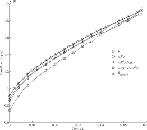
0 0.01 0.02 0.03 0.04 0.05 0.06 0.6 0.8 1 1.2 1.4 1.6 1.8 2x 10 Time [s] Le ng th sc a le [ m ] h <R> <R2>/<R> −<H>*<R2> Rsphere
FIG. 8. Comparison of length scale histories for a terrestrial bubble.
volume-equivalent radii of 12 bubbles have been fitted with high accuracy to Ja√(aL(t – t0)) with t0
the time of growth before the first observation of the bubble with the camera. With 95% confidence interval the results of all bubbles are given by (1T = Tw– Tsat),
terrestrial : J a = 3.22 ± 0.13; 1T = 2.00 ± 0.08◦C; t
leave= 0.088 ± 0.006 s,
microgravity : J a = 1.92 ± 0.13; 1T = 1.19 ± 0.08◦C; t
leave= 0.055 ± 0.02 s.
The time of leaving the nucleation site, tleave, is in the terrestrial case equal to the time of
detachment but has in the microgravity case to be estimated from the observations as the time the bubble starts leaving the site by moving parallel to the wall in downstream direction. Bearing in mind that subcooling of the approaching liquid is 4◦C, a total temperature difference of about 6◦ has to be overcome by the power to the bubble generator in the terrestrial case.
Froude number, equal to Re2/Gr, is for a typical length scale of 5 mm and typical driving
temperature differences of 5 and 6 K estimated to be about 0.7 in on-ground experiments and about 154 in microgravity experiments at minimum (g-jitter of 0.045 m/s2at maximum; expansion
coefficient 2.19 10−31/K). Boundary layer development is therefore affected by mixed convection
in on-ground measurements, but merely by forced convection in microgravity.
On ground, the Jacob number is highest and bubble growth is more rapid. This is confirmed by time histories of length scales measured, as those given by Fig.8. Notice that at later times in this bubble growth history the shape is not that of a truncated sphere as distance h exceeds radius
Rsphere. Since heat transfer rate in terrestrial conditions is higher because of natural convection, a higher superheating of the wall is required to create boiling. It is therefore hard to get identical bubble growth histories in terrestrial and microgravity conditions. The present study applies a force balance analysis to assess the major agents involved and to allow for a prediction of forces in case bubble growth rates in microgravity would be as high as on ground. This analysis is presented in Secs.IV B–IV F.
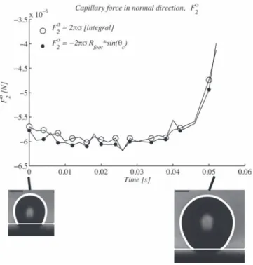
FIG. 9. Comparison of histories of Fσ
2computed in two ways, one with the aid of the contact angle θcand(11)and the
other with the integral equation(10).
The mean detachment radius, Rleave, for the two body force conditions is given by
terrestrial : Rleave = 0.1945 ± 0.0018 mm, contact angle 38◦ ± 4◦; microgravity : Rleave= 0.091 ± 0.016.
Development of an improved criterion for the prediction of the bubble radius at time of leaving the nucleation site is beyond the scope of the present investigation.
B. Assessment of accuracies of various methods to determine force components The important force that attracts a bubble to the wall is the capillary force Fσ
2. Figure9shows
that the integral equation(10)yields about the same values as(11)for a low chosen wall. For a higher chosen wall differences are negligible because of the improved accuracy of the contact angle θcnecessary for(11). The decrease in absolute value of the attracting capillary force with increase
of time in later stages of bubble growth is easily understood from the decrease in apparent contact angle and from(11). The apparent contact angle decreases from about 60◦to about 40◦in the course of time. The variation in the course of time of the capillary force is about the same in both ways of computing it. The accuracy of both ways is expected to be the same.
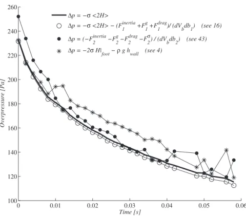
The b1-equation for a bubble attached to a plane wall, the first Euler-Lagrange equation(16),
can be considered as an extended Rayleigh-Plesset equation valid for bubbles of any shape. At each instant of time it contains only one unknown, the overpressure 1p. Figure10shows the time history of the resulting values of the overpressure, at each instant of time given by 1p = −σ h2Hi − (F1inertia
+ F1g+ F1drag) / (∂Vb / ∂b1). The approximation 1p = −σ h2Hi is found to be very close at all
times, as expected. Discrepancies are primarily due to the gravity term F1g. Drag is overestimated
but turns out to be negligible and inertial lift is contributing in later stage of bubble growth, but only little. Although this lift is estimated, using expressions only valid for a truncated sphere, the estimates are sufficiently well to be able to state that the overpressure depends merely on the mean curvature term, −σ h2Hi, and on gravity which is measured via the measured bubble volume. The definition-based approximation 1p = −2σ H|foot− ρLg hwallof(4)depends on the accuracy of the