Measurement of gas diffusion through soils: comparison of laboratory
methods
Suzanne E. Allaire*
a, Jonathan A. Lafond
a, Alexandre R. Cabral
b, and Sébastien F. Lange
a Received (in 2008, May) 1st January 2007, Accepted 1st January 2007First published on the web 1st January 2007
DOI: 10.1039/b000000x
Gas movement through soils is important for ecosystems and engineering in many ways such as for microbial and plant respiration, passive methane oxidation in landfill covers and oxidation of mine residues. Diffusion is one of the most important gas movement processes and the determination of the diffusion coefficient is a crucial step in any study. Five laboratory methods used for measuring the relative gas diffusion coefficient (Ds/Do) were compared using a loamy sand, a porous media
commonly found in agricultural fields and in several engineered structures, such as in landfill final covers. In the absence of macropores, all methods gave rather similar values of Ds/Do. Methods
allowing the study of microscale variability indicated that the presence of macropores highly influenced gas movement, thus the value of Ds/Do, which, near a macropore may be one order of
magnitude higher than in regions without macropores. Repacked columns do not allow the study of heterogenity in Ds/Do. Natural spatial variability in Ds/Do due to water distribution and preferential
pathways can only be studied in large systems, but these systems are difficult to handle. Advantages and disadvantages of each method are discussed.
Introduction
Gas movement through porous media, in particular soils, is a fundamental aspect of many environmental, engineering, ecological, agricultural and biological problems. For example, most plants and microorganisms living in top soils need atmospheric oxygen (O2) ingress by diffusion
otherwise they suffocate. Many of these microorganisms are important for the decomposition of organic matter and contaminants while others impact N and C cycles affecting greenhouse gas (GHG) emissions. Also, fugitive emissions from landfills - which are responsible for nearly 37% of all CH4 emissions in the USA1 and 25% in Canada2 - occur in
part by diffusion of biogas through the cover systems. This process needs to be well understood in order to optimize passive methane (CH4) oxidation by methanotrophic
bacteria, which thrive in the aerobic zone of the cover soil3 and can oxidize between 3 to 90% of the fugitive CH4,
depending on environmental conditions,4 such as nutrient availability5 and oxygen penetration. Many chemical reactions in soils release gases or need gas to take place, such as oxidation of mine residues, which requires O2 input.
Another important aspect to be considered about microbial activity in soils is that the air surrounding the microorganisms must be replaced to eliminate toxic gases and replenish O2.6 Gas diffusion is one of the main
processes responsible for gas movement in soil.7
a Horticultural Research Center, Université Laval, 2480 Hochelaga,
G1K 7P4, Québec, Canada, fax : (418) 656-7871; Tel: (418)656-2131; E-mail: [email protected]
b Dept. Civil Eng., Université de Sherbrooke, Sherbrooke, Qc, Canada,
J1K 2R1
One fundamental step in the study of gas diffusion is the determination of the diffusion coefficient, Ds (m2 s-1) in the
field or laboratory. Werner and co-workers8 found only three review studies9-11 that compared Ds values determined
in situ with those obtained in the laboratory. From the
limited data available, they concluded that in situ and laboratory measurements are equivalent approaches for determining Ds, however, the data were not obtained with
the same soils. They also concluded that studies comparing various methods at the same site are lacking and that evaluation of various methods for heterogeneous and structured media is highly needed. We are not aware of any publication that contradicts Werner and co-workers’s8 conclusion. In addition, in situ methods are costly and, in most cases, do not allow the study of gas movement during winter, and have several draw backs.
Considering the lack of information about Ds for
heterogeneous soils, the fact that there is a good correlation between in situ and laboratory measurements for Ds, and the
relative easiness of performing laboratory tests in comparison to field tests, the goal of this study was to compare five laboratory methods for measuring Ds of a
relatively heterogeneous loamy sand.
Background
Gas diffusion process
Gas-phase diffusion occurs due to collisions between gas molecules. In soils, adjustments to the diffusion coefficient in air are required to account for both the occupancy of a large fraction of the volume by solids or liquids and the non-linearity of the diffusion path in the gas-filled porosity. The adjustments are typically accounted for through a factor multiplied by the
J. Env. Monitoring 10: 1326-1336.
air diffusivity, since the diffusion is still dominated by collisions between gas molecules. When collisions between molecules and solids become significant, due to low pressure or very small pores, Knudsen diffusion can occur.12 Since the soil used in this study has large particles, resulting in large pores, Knudsen diffusion is assumed negligible.
Molecular gas diffusion in soils is described using the 1st
and 2nd Fick’s laws, respectively for steady state (Eq. 1) and
transient (Eq. 2) conditions:
dz
dC
D
q
g s ds=
−
(1) 2 2z
C
D
t
C
g s g a∂
∂
=
∂
∂
θ
(2)where qds is the diffusive flux density in soil (g m-2 s-1), Ds
is the diffusion coefficient (m2 s-1), dCg is the concentration
difference between two points (g m-3), dz is the distance
between two points (m), θa (= Φ-θv) is the air-filled porosity
(m3 m-3), t is the time (s), θv is the soil water content (m3 m -3), Φ (=1-ρa/ρs) is the porosity (m3 m-3), ρa is the bulk
density (Mg m-3), and ρs is the particle density (≈ 2.65 Mg
m-3).
It is often practical to normalize Ds by the gas diffusion in
air, Do (m2 s-1) taken at the same pressure and temperature.
The Ds/Do ratio is lower than one because tortuosity (i.e. the
presence of solid particles and liquid in the pores), is assumed constant for all gases that do not react with the soil particles,13 and depends only on the properties of the air-filled pores of the soil rather than on gas properties.
Relative gas diffusion coefficient relationships
Since measuring methods are time consuming, relationships have been developed for predicting Ds/Do. The simple
methods listed in Table 1 are usually chosen so that diffusion can be calculated from easily measured parameters such as θa and ρa. The relationships vary in their approach,
and are applicable to the type of materials and the range of θv used for their development. Since Ds for a gas in the
liquid phase is about 10 000 times lower than in the gas phase,14 models are usually a function of θa and Φ only.
They also vary according to the importance given to θa and
Φ and in the manner that the restricting factor, which usually accounts for pore tortuosity, constrictivity, and connectivity, is calculated.15 The relationships in Table 1 are widely used in numerical simulations, but their use has some drawbacks since they are sensitive at different levels to errors in the input parameters. In addition, it seems, from the literature, that there is no obvious a priori best relationship for a soil; the choice of a relationship is thus usually supported by a few measured Ds/Do in the material
of interest. To choose the right model, Ds/Do must be well
measured.
Measuring methods
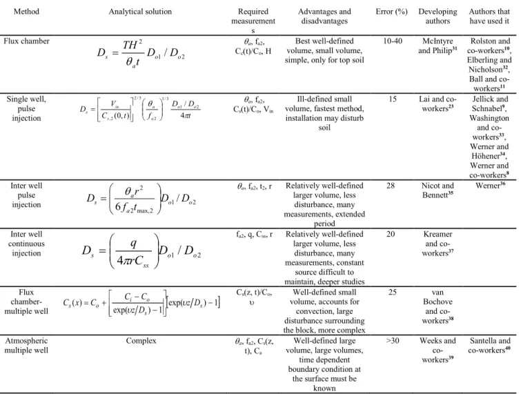
Different methods have been developed to measure Ds in
porous media, both in the field (Fig. 1, Table 2) and in the laboratory (Fig. 2, Table 3). Laboratory methods mainly vary in their initial and boundary conditions and the type of soil core. Also, the hypotheses used to calculate Ds vary
between them.30 During measurements in the laboratory, it is usually assumed that only molecular diffusion occurs, i.e. considering Knudsen diffusion, bubbling, and convection to be negligible.
Fig.1 Scheme of selected field methods for estimating gas diffusion
coefficient.
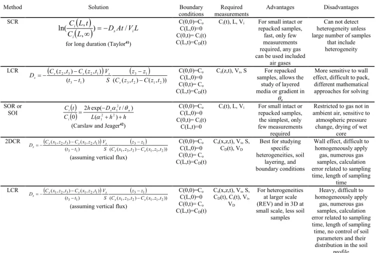
Experimental study
Five laboratory methods for measuring Ds/Do were
compared (Fig. 2, Table 3): (1) small repacked soil columns in a closed system (SCR), (2) long repacked soil columns in a closed system (LCR), (3) small repacked or intact soil columns in an open system (SOI or SOR), (4) large flat soil columns containing macropores in a closed system (2DCR), and (5) large intact monoliths in a closed system (LCI). The five methods are described below.
Fig.2 Scheme of selected laboratory methods for measuring gas
Table 1 Summary of existing simple gas diffusivity relationships
Authors Model Tested material Comments
Buckingham16 2 a o s
D
D
=
θ
Granular material Penman17 a o s D D =0.66θSand, glass bits
Currie18 γθ µ
a o s D
D = Dry granular materials γ and μ vary with material γ varies from 0.8 to 1.0 Millington and Quirk19
3 2 2 Φ = a o s D D θ
Sandy loam Good for different textures of sieved and repacked cores (Jin and Jury20)
Millington and Quirk21
2 3 10 Φ = a o s D D
θ
Different porous materials Not always appropriate for wet soils (Jin and Jury20)
Grable and Siemer22 106 3.36
a o
s D D = −θ
Silty clay loam soil aggregates Micro-diffusion of O2 by electrodes
method Lai and co-workers23 53
a o s
D
D
=
θ
Field method tested withrepacked cores of sandy loam Radial diffusion on field Troeh and co-workers24
υ µ µ θ − − = 1a o s D
D Many types of material μ and υ are empirical Xu and co-workers25 2 51 . 2 Φ = a o s D D θ
Silty clay soil aggregates Ds/Do = 0 for Φ < 0.10 (Cousin12)
Moldrup and co-workers26 3
12 66 . 0 m a a o s D D − Φ
= θ θ Intact and repacked soils combined, m = 3 for intact et m = 6 for Penman and Millington-Quirk models repacked soils
Moldrup and co-workers27
(
)
ba a a a o s D D 2 3 100 100 3 100 0.04 2 + + = θ θ θ
θ θa100 from 0.1 to 0.37 mLoamy-clay soils 3 m-3
Intact cores
b = Campbell28 soil water retention
parameter
Moldrup and co-workers29
100 2 a X o s D D Φ Φ
= θ Intact soils and take into account the θ a100
Three-porosity-encased model (3POE)
(
Φ)
+ = 100 4 1 100 100 log log 2 a a Xθ
θ
θa : Soil air porosity (m3 m-3), Φ: Total porosity (m3 m-3), γ and μ refer to pore shape, diameter, continuity and tortuosity.Table 2 Description of selected field methods for measuring Ds
Method Analytical solution Required measurement
s
Advantages and
disadvantages Error (%) Developing authors Authors that have used it Flux chamber 2 1 2
/
o o a st
D
D
TH
D
θ
=
Cc θ(t)/Ca, fa2o, H , Best well-defined volume, small volume, simple, only for top soil10-40 McIntyre
and Philip31 co-workers Rolston and 10,
Elberling and Nicholson32,
Ball and co-workers11 Single well, pulse injection t D D f t C V D o o a a s in s π θ 4 / ) , 0 ( 1 2 3 / 1 2 3 / 2 2 , = Cs(t)/C θa, foa2, V, in Ill-defined small volume, fastest method, installation may disturb
soil
15 Lai and
co-workers23 Jellick and Schnabel9,
Washington and co-workers33, Werner and Höhener34, Werner and co-workers8 Inter well pulse injection 1 2 2 max, 2 2
/
6
o o a a sf
t
r
D
D
D
=
θ
θa, fa2, t2, r Relatively well-defined larger volume, less disturbance, many measurements, extended period 28 Nicot and Bennett35 Werner 36 Inter well continuous injection 1/
24
o o ss srC
D
D
q
D
=
π
fa2, q, Css, r Relatively well-definedlarger volume, less disturbance, many measurements, constant
source difficult to maintain, deeper studies
20 Kreamer and co-workers37 Flux
chamber-multiple well ( ) exp( ) 1
[
exp( )−1]
− − + = s s o i o s x C CzDC z D C υ υ Cs(z, t)/Co,υ volume, accounts for Well-defined small convection, large disturbance surrounding the block, more complex
25 van Bochove and co-workers38 Atmospheric
multiple well Complex θa, ft), Ca2, Cas(z,
Well-defined large volume, large volumes,
time dependent boundary condition at
the surface must be known >30 Weeks and co-workers39 Santella and co-workers40
Completed and adapted from Werner and co-workers8
θa: air-filled porosity (m3 m-3), fa: fraction of the total mass of the compound in the soil air, Ds: gas diffusion coefficient in the soil (m2 s-1), Do: gas
diffusion coefficient in the air (m2 s-1), Co: applied gas concentration (g m-3), Cs: soil gas concentration (g m-3), Css: steady state gas concentration (g m-3),
Cc: chamber gas concentration (g m-3), H: chamber height (m), Vin: volume of gas injected (m3), q: rate of gas diffusion from source (g s-1), r: distance
from the point source (m), υ: gas apparent velocity (m s-1), t
max: time (s) for maximum tracer concentration at some distance r (m) from the injection point,
Table 3 Description of selected laboratory methods for measuring Ds
Method Solution Boundary
conditions measurements Required Advantages Disadvantages
SCR
( )
(
L)
D At VL C t L C i s i i ) / , , ln( =− ∞for long duration (Taylor41)
C(0,0)=Co
C(L,0)=0 C(0,t)= Ci(t)
C(L,t)=CD(t)
Ci(t), L, Vi For small intact or
repacked samples, fast, only few measurements required, any gas can be used included
air gases
Can not detect heterogeneity unless large number of samples
that include heterogeneity LCR
(
)
(
)
)) , ( ) , ( ( ) ( ) , ( ) , ( 2 1 2 3 1 3 1 3 1 2 3 2 t z C t z C z z S V t t C z t t z C D s s s s s − − − − − = C(0,0)=CC(L,0)=0 o C(0,t)= Co C(L,t)=CD(t) Cs(z,t), Vs, S For repackedsamples, allows the study of layered media or gradient in
θa
More sensitive to wall effect, difficult to pack,
different mathematical approaches for solving SOR or SOI CC
( )
( )
t hL Dhs tha i i + + − = ) ( ) / exp( 2 0 2 2 1 2 1 α θ α (Carslaw and Jeager42)C(0,0)=Co
C(L,0)=0 C(0,t)= Ci(t)
C(L,t)=0
Ci(t), L, Vi For small intact or
repacked samples, the simplest, only few measurements
required
Restricted to gas not in ambient air, sensitive to atmospheric pressure change, drying of wet
core 2DCR ( ) ( ) )) , , ( ) , , ( ( ) ( ) , , ( ) , , ( 2 1 1 2 3 1 1 3 1 3 1 2 1 3 2 1 t z x C t z x C z z S V t t t z x C t z x C D s s s s s s=− −− −−
(assuming vertical flux)
C(0,0)=Co C(L,0)=0 C(0,t)= Co C(L,t)=CD(t) Cs(x,z,t), Vs, S, CD(t), VD
Best for studying specific heterogeneities, soil
layering, and boundary conditions
Wall effect, difficult to homogeneously apply
gas, numerous gas samples, calculation error related to sampling time, length of sampling
time LCR ( ) ( ) )) , , ( ) , , ( ( ) ( ) , , ( ) , , ( 2 1 1 2 3 1 1 3 1 3 1 2 1 3 2 1 t z x C t z x C z z S V t t t z x C t z x C D s s s s s s=− −− −−
(assuming vertical flux)
C(0,0)=Co C(L,0)=0 C(0,t)= Co C(L,t)=CD(t) Cs(x,z,t), Vs, S, CD(t), Ci(t), Vi, VD For heterogeneities at larger scale (REV) and in 3D at small scale, less soil
samples
Heavy, difficult to homogeneously apply
gas, numerous gas samples, calculation error related to sampling time, length of sampling time, no control of soil
parameters and their distribution in the soil
profile VD: volume of the diffusion chamber (m3), Vi: volume of the injection chamber, Vs: soil volume covered by the sampling ports, S: surface of the soil
column (m2), L: length of the soil column (m), C
i(t): gas concentration in the injection chamber at a time t (g m-3), CD(t): gas concentration in the diffusion
chamber at a time t (g m-3), Cs(x,z,t): gas concentration (g m-3) in the soil profile at a certain distance z from the injection point at a distance x from the left
boundary at a time t.
A loamy sand with 77% sand, 17% silt, and 6% clay in the Ap horizon (near the soil surface) and 90% sand, 7% silt,
and 3% clay in the Bf horizon (below) was selected for all
methods. The Ap horizon reached 0.2 m deep while the Bf
reached 0.5 m deep. The number of concretions and the bulk density significantly increased with depth (1.25 to 1.5 Mg m-3). For all methods using repacked columns, composite
samples were taken from the Bf horizon only. For all
methods using intact columns, the samples were taken a few meters apart using the core method43 for small samples and the cylindrical method44 for the large monoliths. For the repacked cores, the soil was sieved through a 2-mm mesh, dried at 105ºC for 24 hours and was hand-packed in fine layers to 1.3-1.4 Mg m-3. In the case of soil detachment
from the casing, bentonite was used to fill up the gap between the soil and the casing. The systems were opened at the end of each test to measure the exact θv,45ρa,43θa,46 and
to observe if cracking, detachment, soil movement, or other anomalies occurred.
The gas injection was similar for all methods with either pulse or continuous injection. The temperature (20ºC ± 2ºC) and atmospheric pressure were maintained constant during the experiment. The systems were gas tight, except for the
upper part of the SOI and SOR methods. Prior to injecting the tracer gas, the systems were flushed with humid air. Either argon or neon was injected. The values of Do at
atmospheric pressure and at 20ºC for Ar and Ne are 2.0 x 10⁻⁵ and 6.5 x 10⁻⁵ m2 s-1, respectively.47,48
The gas sampling technique was the same for all methods. When sampling from soils, 100 µl gas tight syringes (Hamilton Company, Reno, Nevada, USA, no. 81030) were used, whereas for chambers 250 µl gas tight syringes (Hamilton Company, Reno, Nevada, USA, no. 81130) were employed. Gas samples were immediatly inserted into 0.011 L gas tight vials (model 5182-0838, Agilent, Wilmington, DE, USA) with rubber butyl septa (Butyl, lyophilisation, 73828A-21, Kimble Glass Inc., Vireland, NI, USA). Ar or Ne concentrations were measured as soon as possible with a gas chromatograph (6890N, Agilent, Wilmington, DE, USA) equipped with a Headspace autosampler (7694, Agilent), a HP-Molsiv column (19095P-MSO, 30m, Agilent, Wilmington), a TCD detector, and Helium (UHP 5.0, Praxair, Darbury, CT, USA) as the carrier gas. The limit of detection was 0.74 (CV=6.4%) mg L-1 for Ar and
Small repacked column in a closed system (SCR)
This method is also referred to as the two-chamber method.49 The soil was re-moistened until the desired water content was attained, and hand-packed in a 0.10 m-long ABS tube 4 mm thick with a inner diameter of 0.05 m (surface area of 2.1 x 10⁻³ m2). Three replicates were
prepared for each of the three θa (0.3, 0.4, and 0.5 m3 m-3).
A set-up similar to Reible and Shair50 was built (Fig. 2). The column was positioned horizontally in order to limit the creation of a hydraulic gradient, thus moisture redistribution within the column. Ne samples (100 µl) were simultaneously collected from both chambers on several occasions within the first 6 hrs. The Ds was calculated using
the equation given in Table 3. 41,50
Long repacked column in a closed system (LCR)
The same ABS tube, injection and flux chambers were used as for the SCR method, but the soil columns were 0.475 m long (Fig. 2; Table 3). One sample was prepared for the same values of θa mentioned above. Sampling frequency
was previously determined to obtain about 15 sampling events per test. Ar samples were withdrawn simultaneously from both chambers. In addition, gas samples were taken at a 0.05 m interval (8 sampling ports) along the soil columns (Fig. 2). The systems were also horizontally installed and rotated occasionally before measurement to limit the impact of water redistribution. The gas diffusion coefficient was calculated using the finite difference method.51
Small intact or repacked columns in an open system (SOI or SOR)
This method is also known as the Currie Method.49 The 0.077-m long column casing was made of PVC tube with an inner diameter of 0.1 m (surface area of 7.9 x 10⁻³ m2). Soil
θa was controlled by imposing suction with tension tables or
pressure plates after 24 hrs of saturation.52 Therefore, contrary to the other methods presented above, each sample was tested under several θa, starting with the wettest
condition. Any change in soil volume was measured and corrections to θa were made accordingly. The injection
chamber, made of acrylic, had a volume of 7.78 x 10⁻³ m3.
Ar was allowed to diffuse from the chamber through the soil for more than 200 min. Air above the soil core was renewed with low air flow. Ds was calculated using the solution of
Carslaw and Jaeger42 as presented in Rolston53 (Table 3).
Large 2D repacked column with macropores in a closed system (2DCR)
This method (Fig. 2, Table 3) is similar to the methods used in other studies.54,55 The soil columns had the following inner dimensions: 0.6 m wide, 0.025 m thick and 0.6 m high. They were made of 0.012 m thick acrylic. Linear macropores open to the soil surface with a diameter of 0.005 m and a length of 0.3 m were created during packing as in Allaire-Leung and co-workers56 using coarse nylon mesh
fabric held on an aluminium screen After packing, a 0.05 m head of water was applied at the soil surface for 5 min and the soil surface was covered to minimize evaporation. Five days were allowed for equilibrium. Eighty one sampling ports were regularly distributed within the soil sample (Fig. 2). Ne concentrations were measured five times during 24 hrs. The experiment was repeated three times with various macroporosities.
Large monoliths in a closed system (LCI)
Three monoliths were extracted using the method described by Allaire and van Bochove.44 The 0.45 m inner diameter and 0.40 m high casing was made of 0.05 m thick ABS. The samples were constituted of the two horizons, the Ap
horizon at the soil surface and the Bf below. The initial θa of
the monoliths was not controlled. Ne concentration was maintained constant inside the injection chamber. During diffusion, its concentration was measured at a distance of 0.05 m in the vertical direction, and five equally spaced radial positions (Fig. 2). Sampling was completed seven times during 48 hrs. Ds/Do was calculated by finite
differences (Table 3). Ds/Do values given in Fig. 3
correspond to each horizon of each monolith. Lateral flow was not considered in the calculations.
The graphing software for gas distribution in the soil profile was Surfer v.8 (Golden Software, Co, USA) using inverse method for interpolation.
Results and discussion
Comparison between methods
Using the SOI as the baseline for comparison (larger number of tests covering a wide range of θa), it can be
observed in Fig. 3 that the SOR method gave similar values of Ds/Do, over the entire range of θa for which the
experiment was performed. Nonetheless, the tendency is that repacked cores yield slightly higher values of Ds/Do
than intact cores (14% is the greatest difference). This is due to fine cracks that developed during the drying process of the repacked cores. These cracks were comparable and sometime larger than the cracks in the intact cores. In addition, some intact cores had concretions resulting in
Ds/Do lower than in the repacked cores. Values of Ds/Do
obtained with the SCR method followed the same tendency obtained with the baseline method. However, the values with the SCR method were obtained for θa > 0.27 m3 m-3.
The LCI method can also predict Ds/Do values similar to
those by the baseline method, although the comparison only stands for θa up to 0.25 m3 m-3. For θa > 0.25 m3 m-3, high
values of Ds/Do are predicted with the LCR method. This
was probably due to soil loosening. At the end of the experiment, some soil was observed in the flux chamber, indicating that it passed through the screen. This probably occurred because the soil was very dry (about 3% moisture), and the column was horizontally installed and rotated to avoid water redistribution in the column (too much handling). Preferential paths may have developed along the
casing but it is difficult to evaluate the data for evidence of that.
Fig.3 Ds/Do obtained for different air-filled porosity and using different measuring methods.
The 2DCR method resulted in Ds/Do similar to the other
methods when Ds/Do was calculated at points sufficiently
distant (>0.12 m) from macropores, and this is valid for wet and dry conditions (presented together in Fig. 3). The Ds/Do
values from the LCI method were similar with those from the 2DCR method. The values from LCI methods were calculated using the average gas concentration at each height. One value appears high with a Ds/Do of 0.14. It
corresponds to the horizon containing a large earthworm macropore (>4 mm diameter). No such macropore was observed in the other two monoliths used in the LCI method but fine cracks, such as those found in small cores, were observed. Otherwise, differences in Ds/Do between methods
were negligible.
Overall, most of the Ds/Do values presented in Fig. 3 are
comparable with other studies for intact25,29,30 and repacked57,58 soil cores.
Finally, with the exception of the values obtained when macropores were present, all methods predicted similar values of Ds/Do at θa lower than approximately 0.4 m3 m-3
(Fig. 3). For higher θa values, the predicted values are
scattered, which can be partly explained by soil loosening (LCR method) or by the presence of macropores. Therefore, any of these laboratory methods can be used for evaluating
Ds/Do in soils. The choice of a method would depend upon
several factors including simplicity, cost, and soil characteristics (presence of macropores).
Spatial variability
Heterogeneity causing preferential flow (PF) in soil is a key factor for gas flow. Several factors cause PF in soil, such as macropores (cracks and burrows), and heterogeneity in water distribution and pore size. The latter can be caused by vegetation (roots), wet-dry cycles, freeze-thaw cycles, and soil layering. Theoretically, intact cores should better represent gas movement in porous materials than repacked ones, because natural heterogeneity associated with PF is better represented in intact samples.59
Fig.4 Air-filled porosity and gas concentration distributions in a
2D-column after 2 hrs, obtained with the second 2D-column (one open-surface macropore) and with a column without macropores of the 2DCR method.
However, methods using small samples, such as SCR, SOI and SOR yield similar values, as discussed previously. This results from the fact that intact and repacked small samples had similar physical properties at comparable θa and Φ, and
because of the naturally high variability of Ds/Do. In
addition, the small repacked and intact cores contained a similar number of fine cracks and no large features since
large cracks, earthworm burrows, or similar features were avoided for the small intact samples, as is usually done in most studies.
The impact of features like macropores was evident with larger columns such as those used in 2DCR and LCI methods. Indeed, Ds/Do values calculated using the average
concentration in a region around a macropore with the 2DCR was up to 6 times higher (0.07 vs. 0.01) than values obtained away from macropores, for similar θa (Fig. 3).
Figure 4 presents the distribution of θa in 2D columns. θa
was lower around the macropore and behind the wetting front. Normally, one would expect to obtain low gas concentrations in the wet zone (upper part of the column, where θa is lower) since gas movement is much slower in
wet soil than in dry soil (Fig. 3). However, gas concentration did not follow the θa pattern. The distribution
of gas concentration was similar to that expected in a much dryer soil with no macropores (Fig. 4). This can be explained by the gas movement through the macropore and diffusion in all directions, thus laterally giving the impression of a dryer soil.
The impact of soil heterogeneity, including macropore, on gas movement can also be observed in the Fig. 5. After 8 hrs of diffusion, 25% of the surface area at 0.25 m deep had a gas concentration one order of magnitude higher than another 15% of surface area. In addition, one would expect that near the soil surface, gas concentration would be lower since the gas was injected at the lower end of the column. However, 15% of the surface area at 0.25 m deep had a gas concentration higher than 10% of the surface at 0.45 m deep (Fig. 5). This phenomenon was observed in all monoliths. To explain this phenomenon, each column was carefully examined by cutting them into small layers, once gas flux measurements had been completed. The high variability in redox zones (Fig. 5: dark vs. light zones in the Bf horizon at
0.35 m and deeper) is the long-term result of heterogeneity in soil properties. The variability in gas concentration was associated with large concretions, plowing layer, variability in θv, cracks, earthworm burrows, and root channels; but the
most important feature causing this high heterogeneity in gas movement was a large macropore in monolith 2 which resulted in this high Ds/Do value (Fig. 3). The gas moved
upward from the injection chamber and then accumulated right below concretions where the soil has higher density and water content until it reached a PF path. It then moved upward in these PF paths and diffused in all directions in more permeable regions bypassing part of the soil monolith. The importance of PF of gas may become crucial in compacted soils, frozen soils with open macropores, wet soils, and for life forms that live deep in the soil because it allows oxygenation of soil section that would otherwise be anoxic. PF of gas also allows faster elimination of toxic gases in soil toward the atmosphere. It may help, for example, in interpreting the performance in CH4 oxidation
by methanothrophic bacteria in landfill cover materials. This information is also important for interpreting field data, planning spatial measuring frequency, and sampling size.
From this point, the choice of a laboratory method for measuring Ds/Do may, in part, depend on whether one is
interested in variability in Ds/Do or in an overall average of
Ds/Do.
Advantages and disadvantages of the methods
As mentioned previously, similar Ds/Do can be obtained,
irrespective of the method (Fig. 3), when samples are taken away from macrofeatures. It was shown that preferential paths are very important to study gas diffusion in soil. The difficulty of sampling methods to preserve these paths in the cores is a reason for in situ method to be attractive. However, in situ method also have there drawbacks. During installation of the equipement in the field, the disturbance of soil is usually high and may actually be higher than the disturbance in intact cores. In situ measurement is complex because of three dimensional flow. Lateral gas movement is thus often a problem for mass balance. In addition, boundary conditions are often difficult to control or measure which render the Ds/Do calculations less precise. For these
reasons, laboratory method with undisturbed soil cores brought to the laboratory may be as representative to field method when values of small scale Ds/Do is of interest. But
the choice of a method depends on cost, ease of use, and precision, to name a few. In the following, some advantages and pitfalls related to the use of each method are described.
Fig.5 Gas concentration distributions and associated photos in two
large cylindrical monoliths after 8 hrs in different depths obtained with the LCI method.
In the case of small samples, θa can easily be modified by
installing the samples on pressure plates or tension tables. As the soil column becomes longer (LCR), a uniform θa
becomes harder to obtain, particularly when the column is installed vertically. The problems caused by such a gradient may be overcome by withdrawing several gas samples along the column but θa must be measured along the column.
However, this introduces more complexity to the tests. The 2DCR method offered the opportunity to cover a wide range of θa. This could be achieved either through packing at
different θa or by infiltrating water at the soil surface. In
this study, the soil was initially dry and the water did not infiltrate the entire column. As a result, preferential paths were created using macropores. This technique presents the advantage that Ds/Do could be calculated in low and high θa
regions during a single test. Comparatively, the large intact soil cores of the LCI method were too big for any tension tables rendering the control of θa difficult, which in this
experiment, resulted in a narrow range of θa (Fig. 3).
Generally, from the point of view of boundary conditions, a variable (decreasing) concentration boundary condition at the injection level is easier than maintaining a constant concentration in the injection chamber or a zero concentration in the atmosphere or in the flux chamber.
Variable boundary conditions are also less costly because there is no need for instrumentation for controlling the flux. Also, the time required to reach a constant gas concentration in a large injection chamber may be long (Fig. 6) which increases the risk of gas leakage from the injection chamber to the soil column. In addition, a closed boundary condition offers the advantage of a larger choice of tracers. In an open system, the choice is restricted, because gases present in the air are usually not appropriate tracers.
Simplicity and cost are also key factors in choosing a method. The computation of Ds/Do using gas concentration
monitoring obtained from the injection and/or flux chambers only, such as was done in this study in the SCR, SOR, or SOI methods, is relatively fast, easy, and requires only a few samples. For example, about 15 samples are necessary with the SOI or SOR methods to obtain Ds/Do.
However, no information can be obtained as far as gas movement within the soil; only the overall result is computed. The most costly and complex method remains the LCI (large monoliths) method. This is not only associated with the costs related to sampling the core, but also to the large number of gas samples that have to be taken during each test in order to fully profit from the advantages that come with this kind of test.
Error related to packing and sampling small cores may affect
Ds/Do estimate by up to 5%. Homogeneous packing is difficult
especially as the core becomes larger. Higher length to diameter ratio (SCR vs. LCR) would render packing more difficult resulting in decreased homogeneity in θa. Higher ratio
also increases the importance of flows along the boundary (cell walls). Sampling intact cores usually slightly increases soil density44 mostly in less dense soils (e.g. upper horizon). In addition, higher length to diameter ratio usually reinforces the impact of sampling on density44.
Error is also associated to calculations. The precision with instantaneous profile calculations (Table 2) depends upon the time interval between sampling points of the same sampling event. The instantaneous profile method for Ds/Do
calculation requires the gas concentration at four different points (see Equ. in Table 3). The precision with instantaneous profile calculations depends upon the time required to take two samples during a sampling event because the calculations assume instantaneous sampling. Calculations are based upon discrete times assuming instantaneous sampling. It took about 2 min. for two persons for sampling all points in the LCR system, but the time lag between sampling may result in more than 5% error in early time (e.g. 20 min.) after diffusion starts in fast flow condition (e.g. when the soil is dry) and may be as low as 1% after longer time period.
Similar errors associated with the 2DCR and LCI methods arise from the number of samples required for mapping concentration distribution in the profile. For example, it took 25 min. for two people to sample all points in the LCI and 15 min. for two people to sample the entire 81 sampling points of the column of the 2DCR method. It took longer for the large monoliths because sampling was harder to perform, particularly when a stone, a root or other macro
features blocked the needle penetration. If we take an early sampling event as an example (worst case), like 2 hrs after the start of diffusion, and 25 min for sampling all ports with a systematic sampling and using the instantaneous profile calculation, error in estimated Ds/Do may reach up to 30%.
For random sampling (all 81 ports in any order), error in
Ds/Do may reach up to 60%. The error in Ds/Do significantly
decreases as the time lag between two sampling events increases and as the time to sample all the ports during an event decreases. Therefore, the sampling sequence of all points should be planned according to the expected calculations (meaning the four points used for calculating
Ds/Do). When using an optimal sampling system, the error
may be as low as 10%.
Fig.6 Examples of gas concentration in injection and flux chambers
during flux measurement of different methods.
Another source of error for all methods consists in the time required to reach a linear relationship between ln(Cc/Co) vs.
time (Fig. 6). The larger the injection chamber, the higher the error. The methods used for calculating Ds/Do based on gas
concentration in the flux and/or in the injection chambers are also dependent upon precision on the dimensions of the chambers, but these errors together are usually less than 2%. The repacked columns suffer from the fatal flow of not reflecting preferential flow which can dominate the results and cause significant errors. The error in Ds/Do for
macroporous soils may rise up to ten fold.
Conclusion
Gas diffusion measurement is important for many processes in soil. Ds/Do values measured with five laboratory methods
were similar over a large range of air contents. The main differences in Ds/Do between the laboratory methods were
mostly related to the presence of macropores and other soil heterogeneities that some methods can handle while others can not. The choice of the method must then depend on available apparatus, cost, precision and advantages of the methods related to the goal of the study.
Acknowledgments
The authors wish to thank the laboratory work of A.-C. Laliberté, C. Halde, M. Lafontaine, E. Cormier, and V. Juneau. The authors acknowledge the financial support of the Centre SÈVE of the Université Laval, National Science and Research Council of Canada (NSERC), and le Fonds Québécois de la Recherche sur la Nature et les Technologies (FQRNT).
References
1 USEPA, Solid Waste Management and Greenhouse Gases: A
life-cycle assessment of emissions and sinks, United States
Environmetal Protection Agency, 2nd edn., 2002, 136 p.
2 Environment Canada, Inventaire canadien des gaz à effet de serre 1990-2000, 2002, internet link :
http://www.ec.gc.ca/pdb/ghg/1990_00_report/foreword_f.cfm
3 C. Scheutz and P. Kjeldsen, J. Environ. Qual., 2004, 33, 72-79.
4 J. Chanton and K. Liptay, Global Biochem. Cycles, 2000, 14,
51-60.
5 M. Humer and P. Lechner, 7th International Waste Management and Landfill Symposium, Sta Margarita di Pula, Italy, 1999. 6 A. Adamsen and G. King, Appl. Environ. Microbiol., 1993, 59,
485-490.
7 J. Gliński and W. Stępniewski, Soil Aeration and Its Role for
Plants, CRC Press, Boca Raton, Fla, U.S.A., 1985, 229 p.
8 D. Werner, P. Grathwohl and P. Höhener, Vadose Zone J., 2004, 3,
1240-1248.
9 G.J. Jellick and R.R. Schnabel, Soil Sci. Soc. Am. J., 1986, 50,
18-23.
10 D.E. Rolston, R.D. Glauz and G.I. Grundmann, Soil Sci. Soc. Am.
J., 1991, 55, 1536-1542.
11 B.C. Ball, C.A. Glasbey and E.A.G. Robertson, Eur. J. Soil Sci., 1994, 45, 3-13.
12 I. Cousin, Ph.D. Thesis, Université d’Orléans, 1996. 13 K. Shimamura, Soil Sci., 1992, 153, 274-279.
14 E.K. Yanful, J. Geotechn. Eng. ASCE, 1993, 119, 1207-1228.
15 A.H. Weerts, D. Kandhai, W. Bouten and P.M. Sloot, Soil Sci. Soc.
Am. J., 2001, 65, 1577-1584.
16 E. Buckingham, Contributions to our knowledge of the aeration
status of soils. USDA Bureau of Soils, Bulletin 25. Washington.
DC, 1904.
17 H.L Penman, J. Agric. Sci., 1940, 30, 437-462.
18 J. A. Currie, British J. Appl. Phys., 1960, 11, 318-324.
19 R.J. Millington and J.P. Quirk, Transactions of the 7th International Congress of Soil Science, Madison, WI, U.S.A., 1960.
20 Y. Jin and W.A. Jury, Soil Sci. Soc. Am. J., 1996, 60, 66-71.
21 R.J. Millington and J.P. Quirk, Trans. Faraday Soc., 1961, 57,
1200-1207.
22 A.R. Grable and E.G. Siemer, Soil Sci. Soc. Am. Proc., 1968, 32,
180-186.
23 S.H. Lai, J.M. Tiedje and E. Erickson, Soil Sci. Soc. Am. J., 1976,
40, 3-6.
24 F.R. Troeh, J.D. Jabro and D. Kirkham, Goederma, 1982, 27,
239-253.
25 X. Xu, J.L. Nieber and S.C. Gupta, Soil Sci. Soc. Am. J., 1992, 56,
1743-1750.
26 P. Moldrup, T. Olesen, D.E. Rolston and T. Yamaguchi, Soil Sci., 1997, 162, 632-640.
27 P. Moldrup, T. Olesen, P. Schjǿnning, T. Yamaguchi and D.E. Rolston, Soil Sci. Soc. Am. J., 2000b, 64, 94-100.
28 G.S. Campbell, Soil Sci., 1974, 117, 311-314.
29 P. Moldrup, T. Olesen, S. Yoshikawa, T. Komatsu and D.E. Rolston, Soil Sci., 2005b, 170, 854-866.
30 P. Moldrup, T. Olesen, S. Yoshikawa, T. Komatsu and D.E. Rolston, Soil Sci. Soc. Am. J., 2004, 68, 750-759.
31 D.S. McIntyre and J.R. Philip, Aust. J. Soil Res., 1964, 2, 133-145.
32 B. Elberling and R.V. Nicholson, Water Resour. Res., 1996, 32,
1773-1784.
33 J.W. Washington, A.W. Rose, E.J. Ciolkosz and R.R. Dobos, Soil
Sci., 1994, 157, 65-76.
34 D. Werner and P. Höhener, Environ. Sci. Technol., 2003, 37,
2502-2510.
35 J.P. Nicot and P.C. Bennett, J. Environ. Eng. (Resten Va.), 1998, 124, 1038-1046.
36 D. Werner, Ph.D. Thesis, Swiss Federal Institute of Technology, 2002.
37 D.K. Kreamer, E.P. Weeks and G.M. Thompson, Water Resour.
Res., 1988, 24, 331-341.
38 E. van Bochove, N. Bertrand and J. Caron. Soil Sci. Soc. Am. J., 1998, 62, 1178-1184.
39 E.P. Weeks, D.E. Earp and G.M. Thompson, Water Resour. Res., 1982, 18, 1365-1378.
40 N. Santella, D.T. Ho, P. Schlosser and M. Stute, Environ. Technol., 2003, 37, 1069-1074.
42 H.S. Carslaw and J.C. Jaeger, Conduction of heat in solids, Claredon Press, Oxford, UK., 2nd edn., 1959.
43 G.R. Blake and K.H. Hartge, in Methods of soil analysis. Part 1.
Physical and mineralogical method, ed. A. Klute, ASA-SSSA,
Madison, WI, USA., Agron. No. 9, 2nd edn., 1986, ch. 13, pp. 363-376.
44 S.E. Allaire and E. van Bochove, Can. J. Soil Sci., 2007, 86,
885-896.
45 W.H. Gardner, in Methods of soil analysis. Part 1. Physical and
mineralogical method, ed. A. Klute, ASA-SSSA, Madison, WI,
USA., Agron. No. 9, 2nd edn., 1986, ch. 21, pp. 493–544. 46 R.E. Danielson and P.L. Sutherland, in Methods of soil analysis.
Part 1. Physical and mineralogical method, ed. A. Klute,
ASA-SSSA, Madison, WI, USA., Agron. No. 9, 2nd edn., 1986, ch. 18, pp. 443-461.
47 J. Crank, The Mathematics of Diffusion, Oxford Science Publications, Oxford University Press, Great Britain, 2nd edn., 1975, 414 p.
48 R.C. Roberts, in American Institute of Physics Handbook, ed. D. E. Gray, McGraw-Hill, New York, 3rd edn., 1972, ch. 2s, pp. 2-249-2-252.
49 D.E. Rolston and P. Moldrup, in Methods of soil analysis. Part 4.
Physical methods, ed. J.H. Dane and C. Topp, Book series no. 5,
SSSA, Madison, WI, USA., 2002, ch. 4.3, pp. 1113-1140. 50 D.D. Reible and F.H. Shair, J. Soil Sci., 1982, 33, 165-174.
51 R. Naasz, J.C. Michel and S. Charpentier, Soil Sci. Soc. Am. J., 2005, 69, 13-22.
52 A. Klute, in Methods of soil analysis. Part 1. Physical and
mineralogical method, ed. A. Klute, ASA-SSSA, Madison, WI,
USA., Agron. No. 9, 2nd edn., 1986, ch. 26, pp.635-662.
53 D.E. Rolston, in Methods of soil analysis. Part 1. Physical and
mineralogical method, ed. A. Klute, ASA-SSSA, Madison, WI,
USA., Agron. No. 9, 2nd edn., 1986, ch. 46, pp. 1089-1102. 54 S.E. Allaire, S.R. Yates, F.F. Ernst and J. Gan, J. Environ. Qual.,
2002, 31, 1079-1087.
55 S.E. Allaire, S.R. Yates and F.F. Ernst, Vadose Zone J., 2004, 3,
656-667.
56 S.E. Allaire-Leung, S.C. Gupta and J.F. Moncrief, J. Contam.
Hydrol., 2000, 41, 283-301.
57 P. Moldrup, T. Olesen, J. Gamst, P. Schjǿnning and T. Yamaguchi,
Soil Sci. Soc. Am. J., 2000a, 64, 1588-1594.
58 P. Moldrup, T. Olesen, S. Yoshikawa, T. Komatsu and D.E. Rolston, Soil Sci., 2005a, 170, 843-853.