To cite this document:
Pitiot, Paul and Aldanondo, Michel and Vareilles, Elise and Zhang, Linda and
Coudert, Thierry Some experimental results relevant to the optimization of
configuration and planning problems. (2012) In: ISMIS, 4-7 Dec 2012, Macau,
China.
O
pen
A
rchive
T
oulouse
A
rchive
O
uverte (
OATAO
)
OATAO is an open access repository that collects the work of Toulouse researchers and
makes it freely available over the web where possible.
This is an author-deposited version published in:
http://oatao.univ-toulouse.fr/
Eprints ID: 8298
Any correspondence concerning this service should be sent to the repository
administrator:
[email protected]
Some Experimental Results Relevant to the Optimization
of Configuration and Planning Problems
Paul Pitiot1,2, Michel Aldanondo1, Elise Vareilles1, Linda Zhang3, and Thierry Coudert4
1
Toulouse University - Mines Albi, CGI Lab, Albi, France
{paul.pitiot,michel.aldanondo,elise.vareilles}@mines-albi.fr
2
3IL-CCI, Rodez France
3
IESEG School of Management – LEM CNRS, Lille, France
4
Toulouse University - ENI Tarbes, LGP Lab. Tarbes, France
Abstract. This communication deals with mass customization and the associa-tion of the product configuraassocia-tion task with the planning of its producassocia-tion process while trying to minimize cost and cycle time. We consider a two steps approach that first permit to interactively (with the customer) achieve a first product configuration and first process plan (thanks to non-negotiable ments) and then optimize both of them (with remaining negotiable require-ments). This communication concerns the second optimization step. Our goal is to evaluate a recent evolutionary algorithm (EA). As both problems are consi-dered as constraints satisfaction problems, the optimization problem is con-strained. Therefore the considered EA was selected and adapted to fit the problem. The experimentations will compare the EA with a conventional branch and bound according to the problem size and the density of constraints. The hypervolume metric is used for comparison.
Keywords: mass customization, aiding configuration, aiding planning, con-straint satisfaction problem, evolutionary algorithm.
1
Introduction
This paper deals with mass customization and more accurately with aiding the two activities, product configuration and production planning, achieved in a concurrent way. According to the preferences of each customer, the customer requirements (con-cerning either the product or its production) can be either non-negotiable or negotia-ble. This situation allows considering a two-step process that aims to associate the two conflicting expectations, interactivity and optimality. The first interactive step, that sequentially processes each non-negotiable requirement, corresponds with a first configuration and planning process that reduces the solution space. This process is present in many commercial web sites using configuration techniques like automotive
industry for example. Then, a second process optimizes the solution with respect to the remaining negotiable requirements. As the solution space can quickly become very large, the optimization problem can become hard. Thus, this behavior is not fre-quent in commercial web sites. Meanwhile some scientific works have been published on this subject (see for example [1] or [2]) and the focus of this article is on the opti-mization problem. In some previous conferences we proposed an interesting adapted evolutionary algorithm for this problem [3]. However, the presentation was rather descriptive and experimentations were not significant. Therefore, the goal of this pa-per is to compare this algorithm with a classical branch and bound. This initial section introduces the problem and the organization of the paper.
1.1 Concurrent Configuration and Planning Processes as a CSP
Deriving the definition of a specific or customized product (through a set of proper-ties, sub-assemblies or bill of materials, etc…) from a generic product or a product family, while taking into account specific customer requirements, can define product configuration [4]. In a similar way, deriving a specific production plan (operations, resources to be used, etc...) from some kind of generic process plan while respecting product characteristics and customer requirements, can define production planning [5]. As many configuration and planning studies (see for example [6] or [5]) have shown that each problem could be successfully considered as a constraint satisfaction problem (CSP), we have proposed to associate them in a single CSP in order to process them concurrently.
This concurrent process and the supporting constraint framework present three main interests. Firstly, they allow considering constraint that links configuration and planning in both directions (for example: a luxury product finish requires additional manufacturing time or a given assembly duration forbids the use of a particular kind of component). Secondly they allow processing in any order product and planning requirements, and therefore avoid the traditional sequence: configure product then plan its production [7]. Thirdly, CSP fit very well on one side, interactive process thanks to constraint filtering techniques, and on the other side, optimization thanks to various problem-solving techniques. However, we assume infinite capacity planning and consider that production is launched according to each customer order and pro-duction capacity is adapted accordingly.
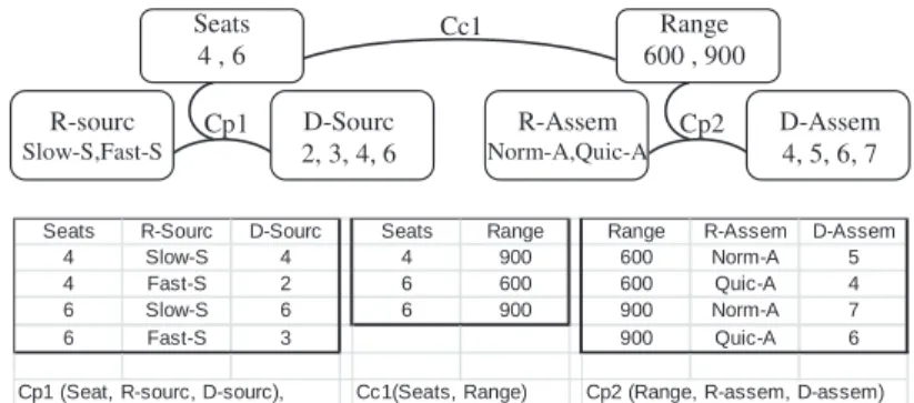
In order to illustrate the addressed problem we consider a very simple example dealing with the configuration and planning of a small plane. The constraint model is shown in figure 1. The plane is defined by two product variables: number of seats (Seats, possible values 4 or 6) and flight range (Range, possible values 600 or 900 kms). A constraint Cc1 forbids a plane with 4 seats and a range of 600 kms. The pro-duction process contains two operations: sourcing and assembling. (noted Sourc and Assem). Each operation is described by two process variables: resource and duration: for sourcing, the resource (R-Sourc, possible resources “Fast-S” and “Slow-S”) and duration (D-Sourc, possible values 2, 3, 4, 6 weeks), for assembling, the resource (R-Assem, possible resources “Quic-A” and “Norm-A”) and duration (D-(R-Assem, possi-ble values 4, 5, 6, 7 weeks). Two constraints linking product and process variapossi-bles
modulate configuration and planning possibilities: one linking seats with sourcing, Cp1 (Seat, R-Sourc, D-Sourc), and a second one linking range with the assembling, Cp2 (Range, R-Assem, D-Assem). The allowed combinations of each constraint are shown in the 3 tables of figure 1. Without taking constraints into account, this model shows a combinatory of 4 for the product (2x2) and 64 for the production process (2x4) x (2x4) providing a combinatory of 256 (4 x 64) for the whole problem. Consi-dering constraints lead to 12 solutions for both product and production process.
Fig. 1. Example of a concurrent configuration and planning CSP model
1.2 Optimizing Configuration and Planning Concurrently
Given previous problem, various criteria can characterize a solution: on the product configuration side, performance and product cost, and on the production planning side, cycle time and process cost. In this paper we only consider cycle time and cost. The cycle time matches the ending date of the last production operation of the confi-gured product. Cost is the sum of the product cost and process cost. We are conse-quently dealing with a multi-criteria optimization problem. As these criteria are in conflict, it is better for decision aiding to offer the customer a set of possible com-promises in the form of Pareto Front.
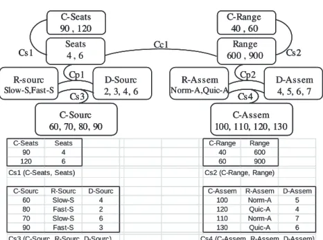
In order to complete our example, we add a cost and cycle time criteria as represented in figure 2. For cost, each product variable and each process operation is associated with a cost parameter and a relevant cost constraint: Seats, Cs1), (C-Range, Cs2), (C-Sourc, Cs3) and (C-Assem, cs4) detailed in the tables of figure 2. The total cost is obtained with a numerical constraint and the cycle time, sum of the two operation durations, is also obtained with a numerical constraint as follow:
Total cost = C-Seats + C-Range + C-Sourc + C-Assem. Cycle time = D-Sourc + D-Assem
The twelve previous solutions are shown on the figure 3 with the Pareto front gather-ing the optimal ones. In this figure, all solutions are present. When non-negotiable requirements are processed during interactive configuration and planning, some of these solutions will be removed. Once all these requirements are processed, the identi-fication of the Pareto front can be launched in order to propose the customer a set of optimal solutions. Seats 4 , 6 Range 600 , 900 R-sourc Slow-S,Fast-S R-Assem Norm-A,Quic-A D-Sourc 2, 3, 4, 6 D-Assem 4, 5, 6, 7 Cp1 Cp2 Cc1
Seats R-Sourc D-Sourc Seats Range Range R-Assem D-Assem 4 Slow-S 4 4 900 600 Norm-A 5 4 Fast-S 2 6 600 600 Quic-A 4 6 Slow-S 6 6 900 900 Norm-A 7 6 Fast-S 3 900 Quic-A 6 Cp1 (Seat, R-sourc, D-sourc), Cc1(Seats, Range) Cp2 (Range, R-assem, D-assem)
Seats 4 , 6 Range 600 , 900 R-sourc Slow-S,Fast-S R-Assem Norm-A,Quic-A D-Sourc 2, 3, 4, 6 D-Assem 4, 5, 6, 7 Cp1 Cp2 Cc1 C-Seats 90 , 120 C-Range 40 , 60 Cs1 Cs2 C-Sourc 60, 70, 80, 90 C-Assem 100, 110, 120, 130 Cs3 Cs4
C-Seats Seats C-Range Range
90 4 40 600
120 6 60 900
Cs1 (C-Seats, Seats) Cs2 (C-Range, Range)
C-Sourc R-Sourc D-Sourc C-Assem R-Assem D-Assem
60 Slow-S 4 100 Norm-A 5
80 Fast-S 2 120 Quic-A 4
70 Slow-S 6 110 Norm-A 7
90 Fast-S 3 130 Quic-A 6
Cs3 (C-Sourc, R-Sourc, D-Sourc), Cs4 (C-Assem, R-Assem, D-Assem)
Seats 4 , 6 Range 600 , 900 R-sourc Slow-S,Fast-S R-Assem Norm-A,Quic-A D-Sourc 2, 3, 4, 6 D-Assem 4, 5, 6, 7 Cp1 Cp2 Cc1 Seats 4 , 6 Range 600 , 900 R-sourc Slow-S,Fast-S R-Assem Norm-A,Quic-A D-Sourc 2, 3, 4, 6 D-Assem 4, 5, 6, 7 Cp1 Cp2 Cc1 C-Seats 90 , 120 C-Range 40 , 60 Cs1 Cs2 C-Sourc 60, 70, 80, 90 C-Assem 100, 110, 120, 130 Cs3 Cs4 C-Seats 90 , 120 C-Range 40 , 60 Cs1 Cs2 C-Seats 90 , 120 C-Range 40 , 60 Cs1 Cs2 C-Sourc 60, 70, 80, 90 C-Assem 100, 110, 120, 130 Cs3 Cs4 C-Sourc 60, 70, 80, 90 C-Assem 100, 110, 120, 130 Cs3 Cs4
C-Seats Seats C-Range Range
90 4 40 600
120 6 60 900
Cs1 (C-Seats, Seats) Cs2 (C-Range, Range)
C-Sourc R-Sourc D-Sourc C-Assem R-Assem D-Assem
60 Slow-S 4 100 Norm-A 5
80 Fast-S 2 120 Quic-A 4
70 Slow-S 6 110 Norm-A 7
90 Fast-S 3 130 Quic-A 6
Cs3 (C-Sourc, R-Sourc, D-Sourc), Cs4 (C-Assem, R-Assem, D-Assem)
Fig. 2. Concurrent configuration and planning model to optimize
Fig. 3. Optimal solutions on the Pareto Front
A strong specificity of this kind of problems is that the solution space is large. It is reported in [8] that a configuration solution space of more than 1.4* 1012 is required for a car configuration problem. When planning is added, the combinatorial structure can become huge. Specificity lies in the fact that the shape of the solution space is not continuous and in most cases shows many singularities. Furthermore, the multi-criteria aspect and the need for Pareto optimal results are also strong problem expecta-tions. These points explain why most of the articles published on this subject (as for
example [9]) consider genetic or evolutionary approaches to deal with this problem. However classic evolutionary algorithms have to be adapted in order to take into ac-count the constraints of the problem as explained in [10]
.
Among these adaptations, the one we have proposed in [3] is an evolutionary algorithm with a specific con-strained evolutionary operators and our goal is to compare it with a classical branch and bound approach.In the following section we characterize the optimization problem and briefly re-call the optimization techniques. Then experimentation results are presented and dis-cussed in the last section.
2
Optimization Problem and Optimization Techniques
2.1 Optimization Problem
The problem of figure 2 is generalized as the one shown in figure 4. The optimization problem is defined by the quadruplet <V, D, C, f > where V is the set of decision riables, D the set of domains linked to the variables of V, C the set of constraints on va-riables of V and f the multi-valuated fitness function. Here, the aim is to minimize both cost and cycle time. The set V gathers: the product descriptive variables and the resource variables. The set C gathers constraints (Cc and Cp). Cost variables and operation dura-tions are deduced from the variables of the set V thanks to the remaining constraints.
Product descriptive variables
Production operation variables
Production cost variables Product cost variables
duration resource Cs Cs Cp cycle time total cost Cc op-1 op-2 ….. Product descriptive variables
Production operation variables
Production cost variables Product cost variables
duration resource Cs Cs Cs Cs Cp Cp cycle time total cost Cc Cc op-1 op-2 …..
Fig. 4. Constrained optimization problem
Experimentations will consider different problem sizes: different numbers of prod-uct variables, different number of prodprod-uction operations and different number of poss-ible values for these variables. Different constraint densities (percentage of excluded combinations of values) will be also considered.
2.2 Optimization Techniques
The proposed evolutionary algorithm is based on SPEA2 [11] with an added con-straints filtering process that avoids infeasible individuals (or solutions) in the arc-hive. This provides the six steps following approach:
1. Initialization of individual set that respect the constraints (thanks to filtering), 2. Fitness assignment (balance of Pareto dominance and solution density) 3. Individuals selection and archive update
4. Stopping criterion test
5. Individuals selection for crossover and mutation operators (binary tournaments) 6. Individuals crossover and mutation that respect constraints (thanks to filtering) 7. Return to step 2.
For initialization, crossover and mutation operators, each time an individual is created or modified, every gene (decision variable of V) is randomly instantiated into its cur-rent domain. To avoid the generation of unfeasible individuals, the domain of every remaining gene is updated by constraint filtering. As filtering is not full proof, incon-sistent individuals can be generated. In this case a limited backtrack process is launched to solve the problem. For full details please see [3].
The key idea of the Branch and Bound algorithm is to explore a search tree but using a cutting procedure that stops exploration of a branch when a better branch has already been found. The first tool is a splitting procedure that corresponds to the selection of one variable of the problem and to the instantiation of this variable with each possible value. The second tool is a node-bound evaluation procedure. The filtering process is used to achieve this task with a partial instantiation and is able to evaluate if the partial instan-tiation is consistent with the constraints of the problem, and, if this is the case, to pro-vide the lower bound of each criterion cycle time and cost. When the search reaches a leaf of the search tree, or complete instantiation, the filtering system gives the exact evaluation of the solution. Thus, the values of leaf solutions can be used to compute the current Pareto front and then to cut remaining unexplored branches that are dominated by any aspect of the Pareto front solution (e.g. the upper bounds of the leaf solution dominate the minimal bounds of the branch to cut).
3
Experimentations
The optimization algorithms were implemented in C++ programming language and interacted with a filtering system coded in Perl language. All tests were done using a laptop computer powered by an Intel core i5 CPU (2.27 Ghz, only one CPU core is used) and using 2.8 GB of RAM. These tests compared the behavior of our con-strained EA algorithm with the exact branch-and-bound algorithm.
3.1 First Experimentation: Problem Size and Constraint Densities
An initial first model, named "full model" is considered. It can be consulted and inte-ractively used at http://cofiade.enstimac.fr/cgi-bin/cofiade.pl select model ‘Aircraft-CSP-EA-10’. It gathers five product variables with a domain size between 4 and 6, six production operations with a number of possible resources between 3 and 25. Without constraints consideration, the solution space of the product model is 5,184, and the
planning model is 96,000. The size of the global problem model is 497,664,000. A second model, named “small model”, has been derived from the previous one with the suppression of a high combinatory task and a reduction of one domain size. This re-duces the planning problem size to 12,000 and global model 6,220,800.
In order to evaluate the impact of constraints density, two versions of each model were produced: one with a "weak density" of constraints (20% of possible combina-tions are excluded in each constraint Cc and Cp) and the other with a "high density" of constraints (50% excluded). These values are frequently met in industrial configu-ration situations. This provides four models characteristics in table 1.
Solution quantity Without constraints Low density High density
Small model 6 220 800 595 000 153 000
Full model 497 664 000 47 600 000 12 288 000
Table 1. Problems characteristics
For the small models, evolutionary settings are tuned to: population size: 50; arc-hive size: 40; Pmut: 0.4; Pcross: 0.8. The ending criterion used is a time limit of half an
hour. For the full models, we adapt settings for a wider search: population size: 150; archive size: 100; Pmut: 0.4; Pcross: 0.8. The ending criterion used is the time required
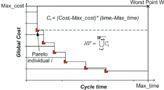
by the BB algorithm. In order to analyze the two optimization approaches, we com-pare the hypervolume evolution during optimization process. Hypervolume metric has been defined in [12]. It measures the hypervolume of space dominated by a set of solutions and is illustrated in Figure 5.
Fig. 5. Hypervolume linked to a Pareto front
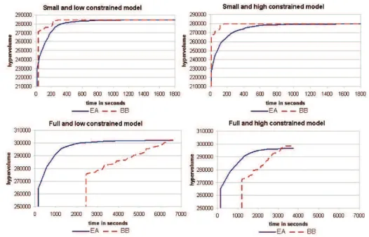
Results are presented in figure 6 where EA curves are average results for 30 execu-tions. Both algorithms start with a lapse of time where performance is null. For the BB algorithm, this corresponds to the time needed to reach a first leaf on the search tree, while for the EA; it corresponds to the time consumed to constitute the initial population.
For the small models (first two curves), the BB algorithm reaches the optimal Pare-to front much faster compared with EA performance. On the other hand, when the problem size increases, the EA is logically better than the BB algorithm on the full model. For example, on the low-constrained model, the BB algorithm took 20 times longer to reach a good set of solutions (less than 0.5% of the optimal hypervolume).
The impact of constraints density could also be discussed. As it can be seen, the BB algorithm performance is improved when the density of constraints is high. In-deed the filtering allows more branches to be cut on the search tree, in such way that the algorithm reaches leaf solutions and, consequently, optimal solutions more quick-ly. The EA performance moves in the opposite way. The more the model is constrained, the more the random crossover operation will have to backtrack to find feasible solutions, and thus the time needed by the algorithm will be consequent.
Fig. 6. First experimentation results
3.2 Experimentations on Problem Size
In order to try to identify the problem size where EA is more suitable than BB, we have modified the low constrained model as follows. We consider now a model ga-thering six product variables and six production operations with three possible values for each, and sequentially add either a product variable and or an operation. The range of study is between 12 and 16 decision variables with three possible values for each. Relevant solution spaces without constraint vary between 1.6*106 and 43*106.
The results are shown in the left part of figure 7. The vertical axis corresponds with the computation time and the horizontal one with the number of decision variables. For BB curves, it shows the time to reach the optimal solution. For the EA curve it shows the time required for nine EA runs over ten to reach the optimal solution. Order of magnitude are close for both around 13 or 14 variables corresponding with a solu-tion space around 2*106 to 5*106 comparable with our previous small model size.
Fig. 7. Experimentation results dealing with problem size
As we already mentioned, industrial models are frequently larger than that. We therefore try our EA approach with a low constrained model with 30 variables and a solution space around 1016. The stopping criterion is "2 hours without improvement". The right part of figure 7 shows that the optimization process has stopped after 48 hours (172800 seconds). It can be noticed that 90% of the final score was obtained after 3 hours and 99% in 10 hours. This allows underlining the good performance of our approach when facing large low constrained problem.
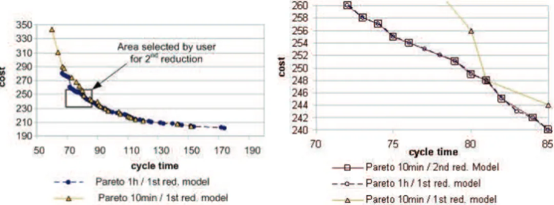
Finally we also try to break optimization in two steps. The idea is: (i) compute quickly a low quality Pareto, (ii) select the area that interest the customer (iii) com-pute a Pareto on the restricted area. The restricted area is obtained by constraining the two criteria total cost and cycle time (or interesting area) and filtering these reductions on the whole problem. The search space is greatly reduced and the second optimiza-tion much faster. This is shown in figure 8 where the left part shows the single step process with 10 and 60 minutes Pareto and the right part shows the restricted area with the two previous curve and the one corresponding with a 10 minutes Pareto launched on the restricted area. It shows that the sequence of two optimization steps of 10 minutes provide a result almost equivalent (only 3 points are missing) to a 60 minutes optimization process.
Fig. 8. Experimentations with a two steps optimization process
0 50000 100000 150000 300000 320000 340000 360000 380000 400000 420000 440000 460000 3h. 10h. 90% 99%
4
Conclusions
The goal of this communication was to propose a first evaluation of an adapted evolu-tionary algorithm that deals with concurrent product configuration and production planning. The problem was recalled and the two optimization approaches (Evolutio-nary algorithm and branch and bound) where briefly presented. Various experimenta-tions have been presented. A first result is that: (i) the proposed EA works fine when the size of the problem gets large compare to the BB, (ii) when problem tends to be more constrained the tendency goes to the opposite. When problem is low constrained (90% of excluded solutions) with 13-14 decision variables with 3 values each, they perform equally. When the problem gets larger, BB cannot be considered and EA can provide good quality results for the same problem with up to 30 variables (around 1016 solutions - 90% unfeasible). Finally some ideas about a two steps optimization process have shown that the proposed approach is quite promising for large problems. These are first experimentation results and we are now working on comparing our proposed EA with some penalty function approaches.
References
1. Hong, G., Hu, L., Xue, D., Tu, Y., Xiong, L.: Identification of the optimal product confi-guration and parameters based on individual customer requirements on performance and costs in one-of-a-kind production. Int. J. of Production Research 46(12), 3297–3326 (2008)
2. Aldanondo, M., Vareilles, E.: Configuration for mass customization: how to extend prod-uct configuration towards requirements and process configuration. Journal of Intelligent Manufacturing 19(5), 521A–535A (2008)
3. Pitiot, P., Aldanondo, M., Djefel, M., Vareilles, E., Gaborit, P., Coudert, T.: Using con-straints filtering and evolutionary algorithms for interactive configuration and planning. In: IEEM 2010, Macao China, pp. 1921–1925. IEEE Press (2010)
4. Mittal, S., Frayman, F.: Towards a generic model of configuration tasks. In: Proc. of IJCAI, pp. 1395–1401 (1989)
5. Barták, R., Salido, M., Rossi, F.: Constraint satisfaction techniques in planning and sche-duling. Journal of Intelligent Manufacturing 21(1), 5–15 (2010)
6. Junker, U.: Handbook of Constraint Programming, ch. 24, pp. 835–875. Elsevier (2006) 7. Aldanondo, M., Vareilles, E., Djefel, M.: Towards an association of product configuration
with production planning. Int. J. of Mass Customisation 3(4), 316–332 (2010)
8. Amilhastre, J., Fargier, H., Marquis, P.: Consistency restoration and explanations in dy-namic csps - application to configuration. Artificial Intelligence 135, 199–234 (2002) 9. Li, L., Chen, L., Huang, Z., Zhong, Y.: Product configuration optimization using a
mul-tiobjective GA. I.J. of Adv. Manufacturing Technology 30, 20–29 (2006)
10. Coello Coello, C.: Theoretical and numerical constraint-handling techniques used with EAs: A survey of the state of art. Computer Methods in Applied Mechanics and Engineer-ing 191(11-12), 1245–1287 (2002)
11. Zitzler, E., Laumanns, M., Thiele, L.: SPEA2: Improving the Strength Pareto Evolutionary Algorithm, Technical Report 103, Swiss Fed. Inst. of Technology (ETH), Zurich (2001) 12. Zitzler, E., Thiele, L.: Multiobjective Optimization Using Evolutionary Algorithms - A
Comparative Case Study. In: Eiben, A.E., Bäck, T., Schoenauer, M., Schwefel, H.-P. (eds.) PPSN 1998. LNCS, vol. 1498, pp. 292–301. Springer, Heidelberg (1998)