Improving the Robustness of Difference of Convex Algorithm in the Research of a Global Optimum of a Nonconvex Differentiable Function Defined on a Bounded Closed Interval

O

pen

A

rchive

T

OULOUSE

A

rchive

O

uverte (

OATAO

)

This is an author-deposited version published in : http://oatao.univ-toulouse.fr/

Eprints ID : 12886

To link to this article : DOI :10.12988/ams.2014.35258

URL : http://dx.doi.org/10.12988/ams.2014.35258

To cite this version : Fadila, Leslous and Marthon, Philippe and

Mohand, Ouanes Improving the Robustness of Difference of Convex Algorithm in the Research of a Global Optimum of a Nonconvex Differentiable Function Defined on a Bounded Closed Interval. (2014) Applied Mathematical Sciences, vol. 8 (n° 1). pp. 1-12. ISSN 1314-7552

Any correspondance concerning this service should be sent to the repository administrator: [email protected]

Improving the Robustness of Difference of Convex

Algorithm in the Research of a Global Optimum of

a Non convex Differentiable Function Defined on

a Bounded Closed Interval

Leslous Fadila Laboratory LAROMAD

Faculty of Science, University Mouloud Mammeri Tizi-Ouzou, Algeria [email protected]

Philippe Marthon

ENSEEIHT-IRIT, University of Toulouse, France [email protected]

Ouanes Mohand Laboratory LAROMAD

Faculty of Science, University Mouloud Mammeri Tizi-Ouzou, Algeria [email protected]

Abstract

In this paper we present an algorithm for solving a DC problem non convex on an interval [a, b] of R. We use the DCA (Difference of Convex Algorithm) and the minimum of the average of two approximations of the function from a and b.

This strategy has the advantage of giving in general a minimum to be situated in the attraction zone of the global minimum searched. After applying the DCA from this minimum we certainly arrive at the global minimum searched.

Keywords: Optimization DC and DCA, global optimization, non convex optimization

1

Introduction

The fminbnd function from MATLAB is a standard method for resolution of a real function minimization defined on a bounded closed interval [a, b] ⊂ R. It realizes a golden section search and parabolic interpolation. It provides us with only a local minimum, not necessarily global if the function is not unimodal [2], [3], [7].

In this paper, we propose an alternate method based on the decomposition of the function in a difference of convex functions (DC) and the application DCA algorithm [6], [8].

The DCA also generally provides a local minimum not necessarily global (or even a critical point) [9], [10], [11].

As the DCA is very sensitive to the choice of the initial point [5], [12], [1], [4] ,we propose not to choose a point of departure. Instead, we minimize the average of two approximations of the function from a and b.

This strategy has the advantage of giving generally a minimum to be located in the attraction zone of the global minimum searched.

We apply the DCA from the minimum found [12], we arrive certainly to the global minimum searched.

2

Problem Formulation

Let us consider the optimization DC problem:

(Pdc) ⇐⇒ min{f (x) = g(x) − h(x), x ∈ [a, b]} f :Rn −→ R nonconvex g :Rn −→ R convex h :Rn −→ R convex

We want to solve the problem Pdc by applying the DCA to the minimum of

the average of the two approximations of f from a and b (MDC).

2.1

Principle of the (MDC) methode

The DCA is very sensitive to the choice of the starting point. [5], [6]

In the case of a minimization a real function defined on [a, b], the minimum found when starting from a will generally be different from that found when

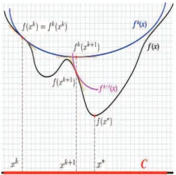
Figure 1: Principle of MDC

starting from b.

We propose not to choose a starting point. Instead we want to minimize the average of two approximations to f from a and b (MDC) let:

min1

2(fk(x, a) + fk(x, b)) with:

fk(x, a) = g(x) − h′(a)(x − a) − h(a)

fk(x, b) = g(x) − h′(b)(x − b) − h(b)

This strategy has the advantage of providing in general a minimum to be located in the attraction zone of the minimum global searched as illustrated by the following example:

2.2

The principle of DCA

Note that DCA works only with DC components g and h [8] , [12].

At the k-th iteration of DCA, h is replaced by its affine minorant hk(x) =

h(xk

) + hx − xk

, yk

i in the neighborhood of xk

.

Knowing that h is a convex function, we have thereforeh(x) ≥ hk(x),∀x ∈ X.

As a result, g(x) − [h(xk ) + hx − xk , yk i] ≥ g(x) − h(x), ∀x ∈ X. That is to say, g(x) − [h(xk ) + hx − xk , yk

i] is a majorant function of function f (x).

Indeed, the surface of fk

can be imagined as a bowl being placed directly above the surface of f; Moreover, the two surfaces touch at point (xk

, f(xk

Figure 2: Principle of DCA

2.3

Proposition 1:

Let g, h two convex functions, differentiable on X. Puting fk

(x) = g(x) − [h(xk + hx − xk , yk i)]. we have [10] : •fk (x) ≥ f (x), ∀x ∈ X. •fk (xk ) = f (xk ). •∇fk (xk ) = ∇f (xk ).

2.4

Proof:

Knowing thad h is convex, h(x) ≥ hk(x), ∀x ∈ X.

Consequently, fk (x) = g(x) − [h(xk ) + hx − xk , yk i] ≥ g(x) − h(x) = f (x), ∀x ∈ X, that is to say: fk (x) = g(x) − [h(xk ) + hx − xk , yk i] ≥ g(x) − h(x) = f(x), ∀x ∈ X, that is to say fk (x) ≥ f (x), ∀x ∈ X. fk (x) = g(xk ) − [h(xk ) + hxk − xk , yk i] = g(xk ) − h(xk ) + 0 = f (xk ). ∇fk (x) = ∇g(x) − yk .

Since g is differentiable, we have: yk

= ∇h(xk ). This is why ∇fk (x) = ∇g(x) − ∇h(xk ). Finally, we obtain ∇fk (xk ) = ∇g(xk ) − ∇h(xk ) = ∇f (xk ).

2.5

Proposition 2:

) − h(xk

)} and {h∗_(yk

) − g∗_(yk

)} decrease and tend to the same limit β which is higher than or equal to the global optimal value α. 2. If (g − h)(xk+1_{) = (g − h)(x}k

) the algorithm stops at iteration k+1, and the point xk

(respectively yk

) is a critical point of g-h (resp. h∗_{− g}∗_).

3. If the optimal value of Problem (P) is finite and if Sequences {xk

} and {yk

} are bounded, then any value of adherence x∗ _{of Sequence {x}k

} (respectively y∗ _{of Sequence {y}k

}) is a critical point of g-h (resp. h∗_{− g}∗_{). [10]}

2.5.1 Remark:

Thanks to Proposition 2, DCA stops if at least one of Sequences {(g − h)(xk

)}, {(h∗_{− g}∗_)(yk

)}, {xk

}, {yk

} converges. In practice, we often use the following stop conditions: • |(g − h)(xk+1_{) − (g − h)(x}k )| ≤ ǫ. • kxk+1_{− x}k k ≤ ǫ.

2.6

Properties of DCA

1- The DCA constructs a sequence {xk

} such that Sequence {f (xk

)} is decreas-ing. This can be easily verified on the figure 2, because xk+1 _{is a minimum of}

fk ( therefore fk (xk ) ≥ fk (xk+1_{) and f (x}k+1_{) ≤ f}k (xk+1_{), as f}k (xk ) = f (xk ). Finally, we have f (xk ) ≥ fk

(xk+1_{) ≥ f (x}k+1_{). This shows that Sequence}

{f (xk+1_{)} is decreasing.}

2- For the boundedness and convergence of DCA, knowing that f:Rn

−→ R∪ {+∞} is bounded from below in Rn

, Sequence {f (xk

)} is also bounded from below. We know that a sequence {f (xk

)} that is decreasing and bounded from below is convergent.

3- When DCA converges to a point x∗_{, this point must be a generalized KKT}

point. this can be easily understood with the help for Figure.2. If we start DCA from a generalized KKT point of f (x∗ _{the figure), then DCA stops}

immediately at this point because it is also a minimum of f∗ _{( the convex}

majorant function defined at point x∗ _{by f (x}∗_{) = g(x) − [h(x}∗_{) + hx − x}∗_{, y}∗_i],

y∗ _{∈ ∂h(x}∗_)).

4- It can be seen, thanks to the figure that DCA has the option to skip certain neighborhoods of local minima. For example, DCA jumps a local minimum between xk

and xk+1 _{then arrives at a neighborhood of the global solution.}

Though we can not always ensure that this phenomenon accurse, we can un-derstand that the performance of DCA is likely to depend on the DC decom-position DC and on the decom-position of the initial point.

3

DCA (DC Algorithm)

Step 1: We search yk

∈ ∂h(xk

). Step 2: We determine xk+1_{∈ ∂g∗(y}k

).

Step 3: If the stop conditions are satisfied then DCA is terminated; Otherwise k=k+1 and we repeat the Step 1.

4

Application of DCA:

4.1

Example 1:

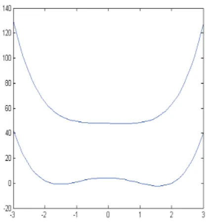
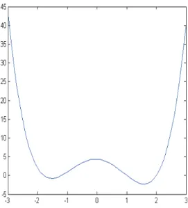
DCA is applied from Point 3 and Point -3, Next we look for the minimum of the two minima in order to find the global minimum.

g(x) = x4_{+ 4, h(x) = 5x}2_{, h′(x) = 10x, y}k = ∇h(xk ) If x0 _{= 3, k = 0, y}0_{= 30} Step 1 x1_{=1,96, y}1 _{= 19, 6} Step 2 x2 _{= 1, 7,y}2 _{= 17} Step 3 x3 _{= 1, 58, y}3_{= 15, 8} such as |x3_{− x}2_{| = |1, 58 − 1, 7| < ǫ}

Then x=1,58 is the optimal solution of the problem (global minimum) with: f(1,58)=-2,25 If x0 = −3, k = 0, y0 = −30 Step 1 x1_{=-1,96, y}1_{= −19, 6} Step 2 x2 _{= −1, 7,y}2 _{= −17} Step 3 x3 _{= −1, 58, y}3 _{= −15, 8} As we have |x3_{− x}2_{| = | − 1, 58 + 1, 7| < ǫ}

Then x=-1,58 is the optimal solution of the problem (global minimum) with: f(-1,58)=-2,25.

Figure 3: Graphical Solution of Example 1 (DCA)

4.2

Remark:

Since f(-1,58)=f(1,58), applying the DCA from -3 or from 3, we arrive at the global minimum because function f is symmetrical.

The standard function fminbnd of MATLAB gives the same solution x=1,58 (global minimum)

4.3

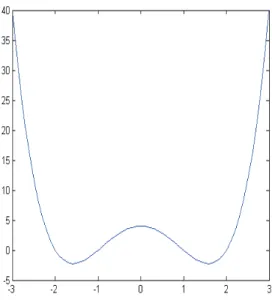
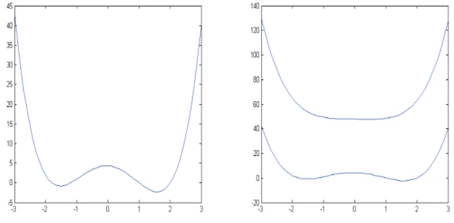
Exampl 2:

We apply the DCA from Point 3 and Point -3. Next, we look for the minimum of the two minima in order to find the global minimum.

g(x) = x4_{+ 0, 48x + 4, 32, h(x) = 4, 84x}2_{, h′(x) = 9, 68x, y}k

= ∇h(xk

) If x0 _{= 3, k = 0}

Step 3 of DCA gives:

x3 _{= +1, 58(nonglobal, localminimum)}

If x0 _{= −3, k = 0}

Step 3 of DCA gives:

x3 _{= −1, 58 (global minimum).}

Fminbnd function of MATLAB gives the solution x=1.58 (non global, local minimum)

Figure 4: Graphical Solution of Example 2 (DCA)

4.4

remark:

In this example we have two minima: One is global and the other is local. So we are Complied to take the minimum of the two, which is a global mini-mum.

The solution of example 2 is: x=-1,58 (minimum global)

The solution of Example 2 with the standard function fminbnd of MATLAB is: x=+1,58 (local minimum).

4.5

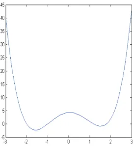
Example 3:

Step 3 of DCA gives the solution x=+1,58 (global minimum). If x0 _{= −3}

Figure 5: Graphical Solution of Example 3 with DCA

The standard function fminbnd of MATLAB gives the solution x=-1,58 (local minimum).

4.6

Remark:

DCA is very sensitive to the starting point. Then we propose in Example 4 to solve the problem of Example 3 with the proposed method, and to obtain the global solution with a single iteration of DCA.

5

Algorithm of the proposed Method (MDCA):

Step O: x0_{= min}1

2(fk(x, a) + fk(x, b)), k = 0.

Step 1: Application of DCA from x0_.

6

Application of the proposed algorithm (MDCA)

6.1

Example 4:

yk

= ∇h(xk

)

We aim to minimize the average of the two approximations of f from -3 and from +3, (fk(x, −3), fk(x, +3)) with: fk(x, −3) = g(x) − h′(−3)(x + 3) − h(−3) fk(x, +3) = g(x) − h′(+3)(x − 3) − h(+3) Therefore: fk(x, −3) = x4+ 28, 56x + 47, 88 fk(x, +3) = x4− 29, 52x + 47, 88 Step:0

Solve the problem convex (P′_{) following:}

(P ′) ⇐⇒ min1

2[fk(x, −3) + fk(x, +3)]

x=0,48 is the solution of Problem (P′₎

Step:1

Application of DCA from x=0,48 x0 _{= 0, 48, k = 0, y}0 _{= 4, 64}

x1 _{is the solution of the convex problem:}

min{x4_{− 16, 11x + 5, 44}}

x=1,58 is the optimal solution (global minimum) of Problem (P)

While the standard function fminbnd of MATLAB gives a local minimum (x=-1,58).

6.2

Remark:

Using the proposed method we did not chose a starting point, instead we want to minimize the average of two approximations of f from 3 and from -3 which will provide a minimum located in the attraction zone of the global minimum. DCA is applied from this minimum, which gives the global minimum searched.

7

Conclusion

We dealt in our work with a particular class of optimization problems, namely: non convex problems (DC).

The strategy of minimizing the average followed by the standard application of DCA has led to the production of the global minimum of function f, while the standard function fminbnd of MATLAB found a non global, local minimum. It now remains to test other examples to better evaluate the pertinence of this strategy, reinforcing the importance of DCA in solving non convex problems.

Figure 6: Solution of Example 4 (DCA)

Figure 7: Solution of Example 4 (MDCA)

References

[1] H.A. Le Thi, N.V. Vinh, et T. Phan Din: A Combined DCA and New Cutting Plane Techniques for Globally Solving Mixed Linear Program-ming, SIAM Conference on Optimization, Stockholm (2005).

[2] Hartman P.: On functions representable as a difference of convex func-tions. Pacific J. Maths. 9, 707-713, (1959).

[3] Horst R., Hoang T.: Global Optimization : Deterministic Approaches, 2nd revised edition. Springer, Berlin,(1993).

[4] Le The H.A: Solving large scale molecular distance geometry problems by a smoothing technique via the gaussian transform and d.c. programming, Journal of Global Optimization, Vol. 27(4), 375-397, (2003)

[5] Nguyen Canh Nam, Le Thi Hoai An, Phan Din Tao : A Branch and Bound Algorithm Based on DC Programming and DCA for Strategic Capacity Planning in supply Chain Design for a New Market Opportunity. Operations rechearch proceedings (2006).

[6] Niu Y.S., Pham Din T.: A DC Programming Approach for Mixed-Integer Linear Programs. Computation and Optimization in Information Systems and Management Sciences, Book Series: Communications in Computer and Information Science, Springer Berlin Heidelberg, 244-253, (2008). [7] Parpas P., Rustem B.: Global optimization of the scenario generation and

Lecture folio selection problems, Computational Science and Its Applica-tions, Lecture Notes in Computer Science, Vol. 3982, 908-917, (2006). [8] Pham Dinh T.: Algorithms for solving a class of non convex

optimiza-tion problems. Methods of subgradients. Fermat days 85. Mthematics for optimization, J.B. Hiriart Urruty (ed.), Elsevier Science Publishers, B.V. North-Holland, (1986).

[9] Pham Din T.: Duality in d.c (difference of convex functions) optimiza-tion. Subgradient methods. Trends in Mathematical Optimization, K.H. Hoffmann et al. (ed.), International Series of Numer Math.84, Birkhauser, (1988)

[10] Pham Dinh Tao and Le Thi Hoai An, Stabilit´e de la dualite lagrangienne en optimisation d.c. (difference de deux fonctions convexes). C.R.Acad. Paris, t.318,SerieI, (1994).

[11] Pham Dinh T., Le Thi H.A., Convex analysis approach to D.C program-ming: Theory, Algorithms and Application. Acta Mathamatica Vietnam-ica, Vol.22 NO .1, 289-355, (1997).

[12] Pham Dinh T., Le Thi H.A.: DC Programming. Theory, Algorithms, Ap-plications: The state of the Art. First International Whorkshop on global Constrained Optimization and Constraint Satisfaction, Nice, October 2-4, (2002)