THESE
THESE
En vue de l'obtention du
DOCTORAT DE L’UNIVERSITÉ DE TOULOUSE
DOCTORAT DE L’UNIVERSITÉ DE TOULOUSE
Délivré par : Institut National Polytechnique de Toulouse Discipline ou spécialité : Dynamique des Fluides
JURY
François-Xavier ROUX Prof. à l’Université Paris 6 Rapporteur Olivier GICQUEL Prof. à l’Ecole Centrale Paris Président du jury
Mouna EL HAFI Maître assist. à l’Ecole des Mines d’Albi Examinateur
Pedro COELHO Prof. à l’IST, Portugal Examinateur
Denis LEMONNIER Directeur de recherche au LET-ENSMA Examinateur
Thomas LEDERLIN Ing. de recherche à Turbomeca Examinateur
Thierry POINSOT Directeur de recherche à l’IMFT Directeur
Ecole doctorale : Mécanique, Énergétique, Génie civil Et Procédés
Unité de recherche : CERFACS
Directeur(s) de Thèse : Thierry POINSOT (Directeur),
Olivier VERMOREL (co-directeur) Présentée et soutenue par Jorge AMAYA
Le 24 Juin 2010 Titre :
Unsteady coupled convection, conduction and radiation
simulations on parallel architectures for combustion applications
Contents
1 Preface xi
2 Introduction xv
3 Introduction xix
I Heat and mass transfers in fluids and solids 1
4 Heat transfer in solids 2
4.1 The Fourier law . . . 3
4.2 Physical properties of solids . . . 3
4.3 The heat equation . . . 4
4.3.1 Initial and boundary conditions . . . 5
4.4 The code AVTP . . . 6
4.5 Analytical and numerical solutions for the transient heat equation . . . 8
4.5.1 The Low-Biot approximation . . . 9
4.5.2 Resolution by the Fourier method . . . 10
4.5.3 Resolution using the Laplace transform . . . 14
4.6 Temperature dependence of the solid properties . . . 17
4.7 Heat transfer in a 3D geometry . . . 18
5 Heat and mass transfer in fluid flows 23
ii CONTENTS
5.1 Thermochemistry of multicomponent mixtures . . . 23
5.1.1 Primitive variables . . . 24
5.1.2 Chemical kinetics . . . 28
5.2 The multicomponent Navier-Stokes equations . . . 32
5.2.1 Turbulent flows . . . 35
5.2.2 Combustion models . . . 41
5.2.3 Near-wall flow modeling . . . 44
5.3 The code AVBP . . . 47
5.3.1 Introduction . . . 47
5.3.2 Overview of the numerical methods in AVBP . . . 48
5.3.3 Boundary conditions . . . 49
6 Radiative heat transfer 50 6.1 Introduction . . . 51
6.2 Basic concepts . . . 52
6.2.1 Principles and definitions . . . 53
6.2.2 Radiative properties of surfaces . . . 59
6.2.3 Radiative flux at the walls . . . 63
6.3 The Radiative Transfer Equation (RTE) . . . 63
6.3.1 Intensity attenuation . . . 63
6.3.2 Augmentation . . . 65
6.3.3 The equation of transfer . . . 67
6.3.4 Integral formulation of the RTE . . . 69
6.3.5 The macroscopic radiative source term . . . 70
6.4 Radiative properties of participating media . . . 71
CONTENTS iii
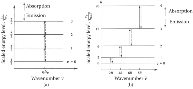
6.4.2 Molecular energy transitions . . . 73
6.4.3 Line radiative intensity and broadening . . . 75
6.4.4 Radiation in combustion applications . . . 78
6.5 Numerical simulation of radiation . . . 81
6.5.1 Spectral models for participating media . . . 81
6.5.2 Spatial integration of the RTE . . . 82
6.6 The code PRISSMA . . . 86
6.6.1 DOM on unstructured meshes . . . 86
6.6.2 Cell sweep procedure . . . 90
6.6.3 Spectral models . . . 92
6.6.4 The discretized Radiative Transfer Equation . . . 109
6.6.5 Parallelism techniques . . . 110
6.6.6 Test cases . . . 115
II Multi-physics simulations on parallel architectures 120 7 Combined conduction, convection and radiation 121 7.1 Introduction . . . 122
7.1.1 Principles of coupling . . . 122
7.1.2 Numerical aspects of coupling . . . 123
7.1.3 Combined heat transfer . . . 124
7.1.4 Technical approach in multi-physics . . . 125
7.2 Fluid-Solid Thermal Interactions (FSTI) . . . 128
7.2.1 The near-wall flow . . . 129
7.2.2 FSTI coupling . . . 139
iv CONTENTS
7.3.1 Background . . . 149
7.3.2 RFTI coupling . . . 150
7.3.3 Effects of radiation on the thermal boundary layer . . . 154
7.4 Solid-Radiation Thermal Interactions (SRTI) . . . 160
7.5 Multi-physics coupling . . . 162
7.5.1 The time scales of heat transfer . . . 162
7.5.2 Multi-physics coupling (MPC) . . . 163
7.5.3 Synchronization of the solvers . . . 164
III Multi-physics simulation of an helicopter combustion chamber 167 8 LES simulation of an helicopter combustion chamber 168 8.1 The study case . . . 169
8.2 Numerical parameters . . . 170
8.3 Quality of the LES simulation . . . 174
8.4 Instantaneous fields . . . 176
8.5 The combustion model and the flame structure . . . 177
8.6 Averaged and standard deviation fields . . . 179
9 Coupled RFTI simulations of an helicopter combustion chamber 186 9.1 Radiation: numerical parameters . . . 187
9.2 Evaluation of the radiation fields . . . 188
9.2.1 The mean absorption coefficient . . . 188
9.2.2 Instantaneous radiative fields . . . 188
9.2.3 Impact of the spectral model for the coupled application . . . 193
9.2.4 Conclusions . . . 198
CONTENTS v
9.3.1 Probe signals . . . 200
9.3.2 Time-averaged fields . . . 202
9.3.3 Averaged radiation vs. radiation of the averaged fields . . . 208
9.3.4 Wall radiative heat flux . . . 212
9.4 Conclusions . . . 213
10 Coupled FSTI simulation of a combustion chamber and a vaporizer injector 215 10.1 Study case . . . 216
10.2 Numerical parameters . . . 217
10.3 Coupling strategy . . . 218
10.3.1 Evolution of the coupled FSTI simulation . . . 220
10.4 Effects on the solid injector . . . 221
10.4.1 Instantaneous temperature fields . . . 221
10.4.2 Time-averaged temperature fields . . . 222
10.5 Effects on the fluid flow . . . 224
10.5.1 Spectral analysis of the unsteady flow . . . 224
10.5.2 Time-averaged flow inside the injector . . . 225
10.5.3 Mean temperature and heat release fields . . . 226
10.5.4 Radial Temperature Function . . . 227
10.5.5 The premixed combustion zone . . . 227
10.6 Conclusions . . . 229
11 Towards multi-physics: LES-DOM-Solid heat conduction coupling in a combustion cham-ber with vaporizer 233 11.1 Introduction . . . 234
11.2 Numerical approach . . . 234
vi CONTENTS
11.4 Impact on the time-averaged radiation . . . 236
11.5 Effects on the temperature of the solid . . . 239
11.6 Impact on the time-averaged fluid temperature . . . 240
11.6.1 Multi-physics vs. uncoupled LES . . . 240
11.6.2 Multi-physics vs. RFTI and FSTI . . . 241
11.7 The RTF profiles . . . 241
11.8 Conclusion . . . 242
12 Conclusions 244 12.1 Engineering accomplishments . . . 245
12.2 Perspectives . . . 246
A The PALM environment 248 A.1 The software . . . 249
A.1.1 Dynamic coupling . . . 249
A.1.2 Parallelism . . . 250
A.1.3 End-point communications . . . 250
A.1.4 Graphical user interface . . . 251
A.2 Palmerization of the codes . . . 251
A.2.1 Unit identification . . . 251
A.2.2 Data manipulation . . . 251
A.2.3 Parallel distribution . . . 252
A.3 The PALM units for multi-physics . . . 252
A.3.1 The unit AVBP . . . 252
A.3.2 The unit PRISSMA . . . 254
A.3.3 The unit AVTP . . . 254
CONTENTS vii
A.4 The PrePALM projects . . . 257
A.5 Cost of coupling . . . 258
A.5.1 Palmerized units without communications . . . 259
viii CONTENTS
Abstract
In the aeronautical industry, energy generation relies almost exclusively in the combustion of hydro-carbons. The best way to improve the efficiency of such systems, while controlling their environmen-tal impact, is to optimize the combustion process. With the continuous rise of computational power, simulations of complex combustion systems have become feasible, but until recently in industrial applications radiation and heat conduction were neglected. In the present work the numerical tools necessary for the coupled resolution of the three heat transfer modes have been developed and ap-plied to the study of an helicopter combustion chamber. It is shown that the inclusion of all heat transfer modes can influence the temperature repartition in the domain. The numerical tools and the coupling methodology developed are now opening the way to a good number of scientific and engineering applications.
Resum´e
Dans l’industrie aéronautique, la génération d’énergie dépend presque exclusivement de la combus-tion d’hydrocarbures. La meilleure façon d’améliorer le rendement de ces systèmes et de contrôler leur impact environnemental, est d’optimiser le processus de combustion. Avec la croissance con-tinue du de la puissance des calculateurs, la simulation des systèmes complexes est devenue abor-dable. Jusqu’à très récemment dans les applications industrielles le rayonnement des gaz et la con-duction de chaleur dans les solides ont été négligés. Dans ce travail les outils nécessaires à la ré-solution couplée des trois modes de transfert de chaleur ont été développés et ont été utilisés pour l’étude d’une chambre de combustion d’hélicoptère. On montre que l’inclusion de tous les modes de transfert de chaleur peut influencer la distribution de température dans le domaine. Les outils numériques et la méthodologie de couplage développés ouvrent maintenant la voie à un bon nom-bre d’applications tant scientifiques que technologiques.
Nomenclature
Accronyms
ACS Asynchronous Coupled Simulations, page 146 DES Detached Eddy Simulation, page 39
DNS Direct Numerical Simulation, page 39 DOM Discrete Ordinates Method, page 85 FSTI Fluid-Solid Thermal Interactions, page 128 LBL Line-by-line, page 81
LES Large Eddy Simulations, page 38 MC Monte Carlo method, page 84 MPC Multi-Physics Coupling, page 162 PCS Parallel Coupling Strategy, page 126 RANS Reynolds-Averaged Navier-Stokes, page 38 RFTI Radiation-Fluid Thermal Interactions, page 148 RTE Radiative Transfer Equation, page 68
RTF Radial Temperature Function, page 207 SCS Sequential Coupling Strategy, page 126 SNB Spectral Narrow-Band, page 81
SRTI Solid-Radiation Thermal Interactions, page 160 TBL Turbulent Boundary Layer, page 132
TRI Turbulence-Radiation Interactions, page 208 WM Wall-Modeled, page 130
WR Wall-Resolved, page 130 Greek symbols
α Absorptance , page 59 [-]
α Nondimensional coupling factor, page 146
α Weighting factor for the mean flux spatial scheme , page 89 [-]
α˜ν Absorptivity , page 64 [-]
βj Temperature exponent of reaction j , page 29 [-]
β˜ν Extinction coefficient , page 65 [m−1]
∆() Absolute difference, page 205
δ() Relative difference, page 205
∆h0f ,k Formation enthalpy of species k , page 24 [J/kg]
x CONTENTS
∆h0f Formation enthalpy , page 27 [J]
∆t Time step , page 7 [s]
∆x Mesh size , page 7 [m]
∆ Stencil size / LES filter size, page 48
δ0L Flame thickness , page 42 [m]
˙
ωk Mass reaction rate of species k , page 29 [kg/(m−3s)]
˙
ωT Heat source term , page 30 [W/m3]
ǫ() Normalized absolute error, page 194
ǫ Emittance , page 59 [-]
γ Polytropic coefficient , page 27 [-]
κ˜ν Absorption coefficient , page 64 [m−1]
λ Thermal conductivity , page 3 [W m−1K−1]
λ Wavelength , page 52 [m]
µ Dynamic viscosity , page 25 [kg.s−1m−1]
ν Frequency , page 52 [Hz]
ν′′,ν′,ν Stoichiometric coefficients , page 29 [-]
νt Turbulent viscosity , page 41 [m2/s]
ω Angular ferquency , page 52 [s−1]
ωdi Directional quadrature weight associated to direction i , page 87 [-]
ω˜ν Monochromatic scattering albedo , page 68 [-]
δ Band average spectral line spacing, page 95
γ Band average of the Lorentz lines half-width, page 95
φ Equivalence ratio , page 31 [-]
φg Global equivalence ratio , page 31 [-]
φ∆˜ν Mean band line shape parametter, page 95
Φ˜ν Scattering phase function , page 66 [-]
λλλ Conductivity tensor , page 3 [Wm−1K−1]
ρ Density , page 3 [kg m−3]
ρ Reflectance , page 59 [-]
ρs Specular reflectance , page 61 [-]
ρd˜ν Diffuse reflectance , page 61 [-]
σ Stefan-Boltzmann constant , page 58 [Wm−2K−4]
σs ˜ν Scattering coefficient , page 65 [m−1]
τ Transmittance , page 59 [-]
τ˜ν Monochromatic optical thickness , page 69 [-]
τi j Viscous stress tensor , page 32 [Pa]
˜ν Wavenumber , page 52 [m−1]
Subscripts and superscripts
0 Relative to the initial condition
τ Relative to the friction properties at the wall ext External/reference quantities
CONTENTS xi
r Quantities related to radiation
s Quantities related to the solid domain
w Wall/interface quantities + Quantities in wall units Roman symbols
˙
m Mass flow rate , page 31 [kg/s]
nj Normal vector of face j , page 88 [-]
q Heat flux vector , page 3 [W/m2]
s Direction vector, page 53
Dk Diffusion coefficient of species k in the mixture , page 34 [m2/s]
Dkt Turbulent diffusion of species k , page 41 [-]
E Efficiency function , page 44 [-]
F Thickening factor , page 44 [-]
Sr Radiative source term , page 71 [W/m3]
κP Planck mean absorption coefficient , page 106 [m−1]
A Mean band absorption , page 93 [-]
I˜ν,i n Averaged intensities crossing the entry faces of a control volume , page 89 [Wm−2Hz−1]
I˜ν,out Averaged intensities crossing the exit faces of a control volume , page 89 [Wm−2Hz−1]
W Mean band equivalent width , page 94 [-]
A Dimensionless average absoption , page 93 [-]
a Thermal difussivity , page 3 [m2s−1]
Aj Pre-exponential factor of reaction j , page 29 [s−1] bN Half-width of a Dopler broadened spectral line, page 77
bN Half-width of a collision broadened spectral line, page 77 bN Half-width of a natural broadened spectral line, page 76
C Specific heat capacity , page 3 [J K−1kg−1]
c0 Speed of light in vacuum , page 51 299792458 [m/s]
Cp Total heat capacity at constant pressure , page 27 [Jkg−1K−1] Cv Total heat capacity at constant volume , page 27 [Jkg−1K−1] Cp,k Heat capacity at constant pressure for species k , page 24 [J kg−1K−1] Cv,k Heat capacity at constant volume for species k , page 24 [J kg−1K−1]
D Diffusion matrix , page 34 [m2/s]
dΩ Infinitesimal solid angle , page 54 [sr]
Dj Projection of the normal of face j on the beam direction j , page 88 [-] Dk
l Diffusion coefficient of species k in species l , page 34 [m2/s] Dk
l Species diffusion coefficient , page 25 [m2/s]
E Total emissive power , page 56 [Wm−2]
E Total energy , page 32 [J]
e Internal energy , page 27 [J]
Eν Spectral emissive power , page 56 [Wm−2Hz−1]
xii CONTENTS
En Energy level of an atom at the nth quantum number , page 73 [eV] Ea j Activation energy of reaction j , page 29 [J/mole]
Ebν Spectral blackbody emissive power , page 56 [Wm−2Hz−1] f (k) k-distribution, page 96
fi Volume force , page 32 [N/m3]
g (k) Cumulative k-distribution, page 96
G˜ν Incident radiation , page 71 [W/m3]
h Convective heat transfer coefficient , page 6 [Wm−2K−1]
h Planck constant , page 52 6,626 10−34[J.s]
h Specific enthalpy , page 27 [J]
hs Sensible enthalpy , page 27 [J]
H˜ν Hemispherical irradiation , page 61 [W/m2]
I Total radiative intensity , page 58 [Wm−2]
Iν Spectral radiative intensity , page 58 [Wm−2Hz−1] I˜ν,P Mean monochromatic irradiation at the center P of a control volume, page 88
Ib ˜ν,P Monochromatic emitted intensity at the center P of a control volume, page 88
k Thermal relaxation coefficient , page 8 [Wm−2K−1]
L Characteristic length , page 9 [m]
Lν Spectral luminance , page 58 [Wm−2Hz−1]
M Pope criterion, page 175
n Number of iterations between two coupling points, page 147
Ndi r Discrete number of directions for the DOM, page 87 NF,O Takeno index, page 178
P Number of allocated processors, page 147
p Pressure , page 26 [Pa]
pa Atmospheric pressure , page 30 [Pa]
pk Partial pressure , page 26 [Pa]
PN N th order spherical harmonic approximation, page 85
qr Radiative energy flux , page 59 [Wm−2]
qνr Spectral radiative energy flux , page 59 [Wm−2Hz−1] R universal gas constant , page 27 8.314 [JK−1mole−1]
R∞ Rydberg constant , page 73 1.097373 107[m−1]
RκP, RT and RIb Emission autocorrelations for TRI, page 210
S Line-integrated absorption coefficient, line strength, page 76
s Stoichiometric coefficient , page 30 [-]
sL Flame speed , page 43 [m/s]
Si j Shear stress tensor , page 40 [m/s2]
T Temperature , page 4 [K]
t Time , page 9 [s]
ui i th component of the velocity , page 32 [m/s]
V Volume , page 26 [m3]
CONTENTS xiii
Vc,t Turbulent correction velocity , page 41 [m/s]
Vik i -th component of the diffusion velocity , page 33 []
W Equivalent line width , page 93 [-]
W Mean molar mas of the mixture , page 24 [kg/mol]
Wk Molar mas of species k , page 24 [kg/mol]
Xk Molar fraction of species k , page 25 [-]
Yk Mass fraction of species k , page 25 [-]
Z Atomic number , page 73 [-]
z Mixture fraction , page 32 [-]
zst Stoichiometric mixture fraction , page 32 [-]
Qj Progress rate of reaction j , page 29 [mol/(m−3s)]
One day there was a storm, with much light-ing and thunder and rain. The little ones are afraid of storms. And sometimes so am I. The secret of the storm is hidden. The thun-der is deep and loud; the lighting is brief and bright. Maybe someone very powerful is very angry. It must be someone in the sky, I think.
After the storm there was a flickering and crackling in the forest nearby. We went to see. There was a bright, hot, leaping thing, yellow and red. We had never seen such a thing before. We now call it “flame”.
One of us had the brave and fearful thought: to capture the flame, feed it a little, and make it our friend.
[...] The flame is ours. We take care of the flame. The flame takes care of us.
1
Preface
One of the most important achievements of mankind is his ability to control fire. And with such power we have been able to fly, take off from Earth and reach space. But the path that lead us to land on Saturn’s biggest moon Titan (Fig. 1.1-a), began around the 15th century B.C. in Babylon, with the invention of the oil lamp (Fig. 1.1-b). At the time Fire was considered one of the four basic elements of nature which, with Water, Air and Earth, flowed through an invisible medium called the Aether. This was the prevailing vision in ancient Greece but it was one shared with Hindus, Buddhist and Chinese, and was first inscribed in the babylonian myth of Enûma Eliš, recovered by Austen Henry Layard in 1849 and published by George Smith in 1979 [239].
After a flourishing era of awakening in science, philosophy, literature, arts and exploration, the clas-sical civilization, the root of our society, felt into an era of obscurantism, marked by the destruction of the last remnants of the Library of Alexandria in the IV century and the death of its last librarian, the mathematician, astronomer, physicist and philosopher, Hypatia, murdered by a Christian mob orchestrated by Cyril, who dragged her from her chariot, tore off her clothes and flayed her flesh from her bones. Her remains were burned and her name forgotten while Cyril was made a saint. Some of the knowledge of the greek scientific tradition of the Alexandrian era was forgotten for almost one millennium. But most of it was lost [223].
It was again, around the XV century, that some of the works of Aristotle, Socrates, Aristarchus, Pythago-ras and other ancient philosophers were rediscovered by a new generation of thinkers in an era of re-naissance. Between them two of the first theoretical physicist1Isaac Newton and Christiaan Huyguens,
1They are considered the first theoretical physicists as they used mathematics in order to explain nature.
xviii Chapter 1: Preface
(a) (b)
Figure 1.1: (a) View of the surface of Titan, Saturn’s largest moon, taken by the ESA Huyguens probe on January 14, 2005. (b) Ceramic oil lamp and its components.
.
established at the end of the XVII century, the starting point in our modern understanding of fire, and in particular one of its most important aspects: light.
Each one had an explanation for light that seemed contradictory2: Newton fervently defended the corpuscular nature of light (which gave origin to one of its most important writings, Opticks [186]) against critics like Robert Hooke and Christiaan Huyguens, who promoted a wave theory of light. A clear mathematical foundation described very well light refraction as a consequence of wave propa-gation, and was more useful to explain the interference patterns observed in the double-stilt experi-ments carried out by Thomas Young [277]. It was Augustin-Jean Fresnel who, at the beginning of the XIX century, rediscovered Huyguens results and showed that the wave theory of light is not in con-tradiction with the linear propagation of light (one of Newton’s arguments against the theory). Today the model that explains refraction and diffraction of light is called the Huyguens-Fresnel principle. However, the corpuscular/wave controversy remained open until the end of the XIX century.
To understand the origin light it is indispensable to understand electromagnetic theory. Michael Fara-day was born in 1791 and from 1804 to 1811 he worked as a book binder in a library. There he became aware of the scientific literature and got versed in some specific topics while developing very good handicraft skills. At the age of 20 he became assistant of chemist Humphry Davy of the Royal Insti-tution. He became a good laboratory employee, and eventually instruments supervisor, laboratory director and finally in 1833 professor of chemistry at the Royal Institution of Great Britain.
His great ability to setup precise and good experiments allowed him to understand the intricate re-lationship between electricity and magnetism. In particular he is at the origin of the induction of an electric current by the motion of a magnet, which finally derived in great technical advances, as the
xix
electrical engine, the electrical generator, public electricity and wire communications, but also lead to the concept of electric and magnetic fields, inspiring James Clerk Maxwell who in 1873 published his most famous work A treatise on electricity and magnetism [165].
Maxwell found a close link between the magnetic and the electric fields. Applying these results to the particular case of a linearly propagating harmonic electric wave, he deduced that there exists an associated perpendicular magnetic wave. In the vacuum the propagation speed of this coupled wave perfectly matches the speed of light. Light is an electromagnetic wave. Some years after Maxwell’s death Heinrich Hertz showed that at some frequencies these waves become invisible but are still de-tectable using measuring instruments. Hertz is the father of VHF and UHF radio waves, and light is only one small part of a greater electromagnetic wave spectrum.
But still some experiments showed that light behave like a particle. It was only after the quantum rev-olution of the beginning of the XX century that the final answer came in the strangest form. Through the work of Max Planck, Albert Einstein, Louis de Broglie, Arthur Compton and Niels Bohr, the cur-rent scientific consensus holds that all particles (including light) have both wave and corpuscular properties.
Fire is also build on interacting particles. It is the energy stored inside the chemical compounds of a molecule of fuels that generates the necessary energy in the first place to produce heat and light. It was the medieval Arab and Persian scholars who first introduced a precise observation and controlled experimentation, which lead to the discovery of numerous chemical substances.
The most influential Muslim chemists were J¯abir ibn Hayy¯an (d. 815), al-Kindi (d. 873), Al-R¯az¯ı (d. 925), al-B¯ır¯un¯ı (d. 1048) and Alhazen (d. 1039). The works of J¯abir became more widely known in Europe through latin translations. The emergence of chemistry in Europe during the XV century was mainly motivated by the rise in the demand for medicines. Over time, the initial alchemy approach was replaced by a more strict and scientific method. Paracelsus in he XVI century rejected the 4-elemental theory and, with only a vague understanding of his chemicals and medicines, formed a hybrid of alchemy and science. The systematic and scientific revolution promoted by Sir Francis Bacon and René Descartes inspired philosophers like Robert Boyle to perform analytical scientific studies in domains like combustion, oxidation and respiration.
It was however Antoine Lavoisier, who developed the theory of conservation of mass in 1783, that ad-vanced the oxygen theory of combustion (“the acid principle” or “the oxygen principle” derived from the greek oxus=acid). The detailed experimental analysis carried out by Levoisier, was completed by the work of Claude Berthollet, Guyton de Morveau and Antoine de Fourcroy who helped in the refor-mulation of a consistent chemical nomenclature. A complete compendium of such enterprise can be found in the 1787 Traité élémentaire de chimie by Levoisier, the father of modern chemistry.
Finally, the transport of the different chemical elements in a continuum medium is the subject of the fluid dynamics, which in the XVIII and XIV century was a subject of controversy among the physicists. In 1757 Leonhard Euler published his work on the general principles of fluid motion. Many modern applications still rely on Euler’s mathematical model of inviscid flows. But during the decades that
fol-xx Chapter 1: Preface
lowed Euler’s discovery experiences and theoretical analysis showed that improvements of the model where necessary. Almost one century later Claude Navier published a mathematical derivation of the equations of motion of incompressible viscous fluids. His model, altough accurate, was obtained using a wrong analysis of the interaction forces between particles. It was Jean-Claude Barré de Saint-Venant who established a correct physical framework for the derivation of the modern Navier-Stokes equations, interpreting the multiplying factor of the velocity gradient as a viscous coefficient, and identifying such product as the viscous stresses acting within the fluid because of friction. It’s still uncertain why the name of Saint-Venant has never been associated with the equations of motion of viscous fluids.
The equations were independently derived by George Stokes, who worked as the Lucasian chair of mathematics at Cambridge during most of the second half of the 19th century. His expertise on fluid mechanics was mainly inspired by his work on the properties of light, the searching for an explanation of it’s movement within the ether and the study of the motion of pendulum. The monumental contri-butions of Stokes on the understanding of friction in viscous flows is still honored with the inclusion of his name in the Navier-Stokes equations of fluid motion.
Building a theory that explains how a candle works required the tireless work of the most prominent scientists, some of which, sometimes without knowing, became prolific scientists in all the areas re-lated to combustion (chemistry, electromagnetism, fluid dynamics, heat transfer, etc.):
Atom by atom, link by link, has the reasoning chain been forged. Some links too quickly and to slightly made have given way, and replaced by better work; but now the great phenomena are known, the outline is correctly and firmly drawn, cunning artists are filling the rest, and the child who masters these Lectures knows more of fire than Aris-totle.
2
Introduction
La combustion est la science qui étudie, à l’aide de la chimie, la mécanique des fluides et le transfert de chaleur, les mécanismes impliqués dans le dégagement d’énergie due à l’oxydation exothermique de molécules de combustible. Dans des applications industrielles la combustion est communément utilisé pour le dimensionnement de machines pour la transformation efficace d’énergie chimique en travail mécanique en utilisant la théorie des cycles thermodynamiques.
Une bonne connaissance théorique des processus sous-jacents de la combustion a été développée dans les dernières décennies, néanmoins, pour des applications industrielles, les interactions non-linéaires entre les différents phénomènes physico-chimiques font presque impossible une étude an-alytique du processus de combustion qu’en générale incluent une géométrie complexe et un écoule-ment turbulent. Une réponse à ce problème a été présenté à la fin de la seconde guerre mondiale: pour résoudre les équations qui déterminent le comportement des bombes nucléaires, Stanislaw Ul-man et John von NeuUl-mann ont eu recours à la simulation numérique et aux ordinateurs. Le labo-ratoire de Los Alamos en Californie a été le berceau de la plupart des méthodes numériques utilisés actuellement pour la résolution numérique du transfert de chaleur et de la dynamique des fluides. Pendant la seconde moitié du 20ème siècle et le début du 21ème, les simulations par ordinateur ont été utilisées pour résoudre des problèmes extrêmement complexes et on permis d’étudier, des prob-lèmes physiques fondamentaux comme la turbulence, le transfert de chaleur, les couches limites, la dynamique moléculaire, la chimie et le rayonnement entre autres. Aujourd’hui les simulations par ordinateur sont utilisés pour étudier et valider systèmes complexes comme celui visé par ce travail: les chambres de combustion aéronautiques.
xxii Chapter 2: Introduction
Une forte augmentation de la puissance de calcul a été observée ces dernières années et elle est prin-cipalement due à la réduction dans la taille des transistors des processeurs et à la distribution des tâches sur plusieurs unités de calcul. Les simulations sur des architectures parallèles ont montré des résultats étonnants, comme ceux présentés par Wolf et al. [271] et Boileau et al. [17]. Ces simulations incluent plusieurs modèles avancés pour la turbulence, le changement de phase des hydrocarbures, la cinétique chimique et la stabilité numérique, mais elles n’ont pas tenu encore en compte quelques uns des phénomènes physiques les plus importants, car leur inclusion restait encore très coûteuse. Dans une chambre de combustion la chaleur peut être transmise par rayonnement, par conduction et par convection. Les interactions thermiques entre le solide et le fluide sont très fortes: la température de la structure impose un flux thermique à l’interface entre les deux milieux. De l’énergie peut être rayonnée par ce même solide et par les zones chaudes du gaz quand ils se trouvent à haute tempéra-ture, et peuvent aussi absorber de l’énergie quand leur température est basse. De plus, les gradients de température dans le fluide imposent un flux de chaleur vers les parois. Finalement, les propriétés radiatives du fluide dépendent des propriétés thermochimiques du mélange. En bref, chaque mode de transfert encadre l’évolution des autres modes.
Dans ces dernières années, différents équipes de recherche ont aperçu la nécessité croissante d’inclure tous les modes de transfert de chaleur pour l’étude des applications en combustion. Concernant l’interaction entre le rayonnement et le fluide Schmitt et al. [230] et Gonçalves dos Santos et al. [64] ont montré que le rayonnement peut modifier la dynamique de flamme. Des simulations numériques sur l’interaction rayonnement-turbulence (Turbulence-Radiation Interaction: TRI) ont été réalisées (voir Coelho [45] pour avoir une synthèse des travaux réalisés dans ce domaine), les interactions en-tre la combustion et le rayonnement ont été étudiées par Kounalakis et al. [139], Adams et al. [3], Desjardin et Frankel [60], Giordano et Lentini [87], Wu et al. [272, 273] Deshmukh et al. [58, 59], Narayanan et Trouvé [185], et des analyses sur l’influence du rayonnement sur des systèmes de com-bustion aéronautiques ont gagné grande couverture par les travaux de Lefebvre [147], Mengüç et Viskanta [263], et plus récemment par Bialecki et Wecel [15] et Paul and Paul [194].
Concernant l’interaction Fluide-Solide pour des applications en combustion des travaux sur l’impact du transfert de chaleur entre les gaz de combustion et les vannes de guidage en sortie de chambre ont été réalisés par Grag [84], Wang et al. [266], Kassab et al. [129], Mazur et al [167], and Duchaine et al. [67]. Des méthodes pour les échanges entre ces deux milieux ont été largement étudiées par Errera et al. [74, 75], Chemin [40], Roux [221] et Châtelain [39].
La littérature au sujet des interactions entre le rayonnement et la combustion et entre la convection et la conduction, est récente. Dans ce travail un des objectifs est d’approfondir l’étude des effets combinés des trois modes de transfert de chaleur (convection, conduction, rayonnement) appliqués à une géométrie complexe tout en tenant en compte de la combustion turbulente. La puissance de calcul actuelle a atteint un point où un tel type de simulation parallèle peut être réalisée. Ce travail demande donc la connaissance de trois domaines de la physique et d’un travail de développement de nouveaux outils numériques. Le principal objectif de cette thèse est d’explorer comment les architectures parallèles modernes et les outils de couplage peuvent être utilisés pour réaliser des
xxiii
simulations couplées instationnaires multi-physiques.
En se basant sur ces artchitectures parallèles, trois codes qui résolvent les trois modes de transfert de chaleur sont employés pour analyser les effets couplés en combustion. Le but est de ainsi de s’attaquer aux aspects scientifiques et d’ingénierie nécessaires pour un tel type d’étude. Dans le do-maine scientifique, chaque phénomène de transfert doit être étudié et les outils numériques em-ployés pour leur résolution spatio-temporelle doivent être évalués de façon indépendante.
Finalement, l’utilisation de simulations couplées doit montrer qu’il existe une amelioration de la pré-diction du comportement du système par rapport aux simulations non couplées. En particulier il est important de déterminer dans quels aspects les simulations couplées présentent des prédictions plus exactes, et quand est-ce qu’un tel type de simulation n’est pas nécessaire.
Les simulations couplées peuvent être utilisées pour l’étude du transfert de chaleur dans les couches limites turbulentes, pour l’étude de la structure de flamme et son stabilité, pour l’étude de la dy-namique du fluide et de la distribution de température dans le domaine de calcul.
Afin de satisfaire les besoins industriels une simulation couplée doit répondre aux exigences suiv-antes:
• Géométries complexes: pour des applications en aérodynamique interne les géométries com-munément étudiées sont très complexes. Elles peuvent inclure différentes zones d’injection de différentes tailles et dans le cas des chambres de combustion comportent une forme toroïdale caractéristique. Les codes doivent être capables de manipuler un tel type de mailles, qui pour la plupart sont composés d’éléments hybrides (tétraèdres, hexaèdres, pyramides, etc.).
• Temps de restitution: même si les Simulations aux Grandes Echèlles (SGE) ne sont pas la norme dans l’industrie, elles sont en train de devenir de plus en plus populaires grâce à leur ef-ficacité pour prédire des phénomènes instationnaires. La croissance de la puissance de calcul et un accès plus aisé à des super calculateurs sont des arguments qui permettront aux indus-triels de se tourner dans les années à venir vers la SGE. Néanmoins, le temps de restitution de cette méthode est encore très grand et demande encore beaucoup d’heures de travail humain. Les simulations couplées doivent présenter des temps de restitution comparables à celles mon-trées par la SGE seule.
• Portabilité: les outils de simulation doivent être faciles à transporter d’un ordinateur à un autre, insouciant de l’architecture et du système d’exploitation. Les simulateurs doivent demander une intervention minimale quand ils sont installés sur des nouveaux systèmes. Dans le cas des simulations couplées cette tâche demande une politique de développement, car au lieu d’un seul code les applications multi-physiques font intervenir de plusieurs codes, unités de communication et logiciels de couplage qui doivent évoluer de façon simultanée.
• Ergonomie: un code qui présente une clarté de fonctionnement est plus facile à être pris en main, est plus fonctionnel, efficace et plus agréable utiliser. Un des problèmes majeurs de la
xxiv Chapter 2: Introduction
computation scientifique et de sa mise au service de l’industrie est la négligence des inter-actions entre l’utilisateur et le logiciel. Pour des applications dans lesquelles plusieurs codes doivent coexister il est essentiel de garder une interface consistante entre l’utilisateur et les dif-férents codes.
Pour palier à ces besoins d’ingénierie, les outils numériques utilisés doivent être évalués et optimisés, et d’autres doivent être développés. Les objectifs particuliers de ce travail de thèse dans ce domaine concernent:
• l’évaluation des performances du code de conduction AVTP pour réaliser des simulations tran-sitoires,
• le développement et optimisation du code radiatif PRISSMA pour des applications couplées, • la mise en place du software permettant la distribution de ressources et la synchronisation des
trois codes de calcul AVBP (pour la SGE), AVTP (pour la conduction) et PRISSMA (pour le ray-onnement) à l’aide du coupleur PALM,
• la réalisation d’une simulation couplée d’une chambre de combustion aéronautique, incluant les phénomènes instationnaires de la combustion turbulente, la conduction de chaleur dans la structure et des modèles détaillés de rayonnement électromagnétique.
Ce document est divisé en trois parties majeures: dans la première partie une introduction à cha-cun des modes de transfert est présentée. Une attention particulière est donnée à la théorie du ray-onnement électromagnétique et aux méthodes numériques employés pour résoudre l’équation de transfert radiatif sur des architectures parallèles. Dans la deuxième partie une description des effets thermiques couplés et des méthodes développées pour résoudre leurs interactions instationnaires sont présentés. Finalement, dans la troisième partie, les outils développés dans les sections précé-dentes sont utilisés pour réaliser le couplage instationnaire d’une chambre de combustion d’hélicoptère et pour étudier les effets des interactions thermiques Fluide-Rayonnement, Solide-Fluide et Multi-Physiques.
3
Introduction
Combustion is the science that combines chemistry, fluid dynamics and heat transfer in order to explain the mechanisms of energy release due to the exothermal oxidation of fuel molecules. In in-dustrial applications combustion is used to design efficient tools that transform chemical energy into mechanical work using a thermodynamic cycle.
A good understanding of all the underlying processes in combustion has been acquired over the last decades. However, in industrial applications there are non-linear interactions between the different physicochemical phenomena, making almost impossible to develop an analytical study of a com-bustion process involving a complex geometry and a turbulent flow. One answer to this problem was given by the time of World War II, when the resolution of the equations describing a complex system as the explosion of a nuclear bomb was carried out by Stanislaw Ulman using simulations with John von Neumann digital computers. Los Alamos Laboratory was the birth place of many of the modern numerical methods used in heat transfer and fluid dynamics.
During the second half of the XX and the beginning of the XXI centuries, computer simulations have been used to resolve extremely complex problems and gave the opportunity to study, from a new point of view, fundamental scientific problems such as turbulence, heat transfer, boundary layer the-ory, molecular dynamics, molecular chemistry and radiation among others. Today computer simula-tions are used to study and validate complex systems as the one targeted in this work: the unsteady simulation of an aeronautical combustion chamber.
The increment in computational power has been mainly achieved by reduction in the transistor size and by the distribution of the tasks over many different process units, what is called parallel
xxvi Chapter 3: Introduction
puting. Simulations of combustion on parallel architectures have shown incredible results, as in the case of Wolf et al. [271] and Boileau et al. [17]. Such simulations include many complex models for turbulence, phase change, chemistry and numerical stability, but still do not take into account some important physical phenomena, as the simulation of such systems may be very expensive.
In a combustion chamber heat can be transfered by radiation, conduction and convection. The ther-mal interactions between the solid and the fluid are closely related: the temperature of the solid struc-ture imposes a heat flux to the fluid, while radiation emitted by the solid wall and by the hot spots in the gas is absorbed by cold zones in the fluid and the structure. In addition, the temperature gradients in the fluid impose a heat flux to the walls and finally the radiative properties of the fluid depend on the thermochemical properties of the mixture. In summary each transfer mode bounds the evolution of the others.
In the last years however, different scientific teams have acknowledged the necessity to include dif-ferent heat transfer modes for the study of combustion applications. Concerning the Fluid-Radiation interaction Schmitt et al. [230] and Gonçalves dos Santos et al. [64] showed that radiation can mod-ify the flame dynamics. Advances in numerical simulation include the study of the Turbulence-Radiation Interactions (Coelho [45] gives a good synthesis of the state of the art in TRI), the inter-actions between combustion and radiation of Kounalakis et al. [139], Adams et al. [3], Desjardin et Frankel [60], Giordano et Lentini [87], Wu et al. [272, 273] Deshmukh et al. [58, 59], Narayanan et Trouvé [185], and the analysis of radiation effects on aeronautical combustion systems which have receive wide coverage by Lefebvre [147], Mengüç et Viskanta [263], and more recently by Bialecki et Wecel [15] and Paul et Paul [194].
In the complementary field of Fluid-Solid interaction, work has been done on the impact of hot com-bustion gases on the guiding vanes at the exit of the comcom-bustion chamber by Grag [84], Wang et al. [266], Kassab et al. [129], Mazur et al [167], and Duchaine et al. [67]. Other fundamental principles on Fluid-Solid Thermal Interactions (FSTI) have been studied by Errera et al. [74, 75], Chemin [40], Roux [221] and Châtelain [39].
Scientific literature on the interaction between radiation and combustion (Radiation-Fluid) and be-tween convection and conduction (Fluid-Solid) is recent. In the present work our aim is to go one step further and study the combined effect of the three heat transfer modes, conduction, convection and radiation applied to an industrial complex geometry, while resolving the unsteady turbulent combus-tion. The current available computational power has reached a point where such parallel simulations can be performed. This task demands the knowledge of three different areas of physics and involves the development of new numerical tools. The main objective of the present work is to explore the possibilities of modern parallel architectures and coupling methods to achieve unsteady Multi-Physics Coupled (MPC) simulations.
Taking advantage of the parallel architectures, three codes that solve the three heat transfer modes are employed to analyze the coupled effects in combustion. The goal is then to tackle both the scientific
xxvii
In the scientific area, each independent heat transfer mode must be understood, and the numerical tools developed must show a good prediction of the spatial and temporal evolution of each indepen-dent system. Next, the interactions between the different transfer modes must be analyzed, and the effects of one subsystem on the other must be presented (how does radiation affect convection for example).
Finally, the use of coupled simulations must show that there exists an advantage in the prediction of the system’s behavior against uncoupled simulations. In particular it is important to determine in which aspects coupled simulations can provide more accurate predictions, and when they are not necessary. Coupled simulations can be used to study the effects on the heat transfer in the turbulent boundary layer, the flame structure and its stability, the flow dynamics and the temperature distribu-tion in the studied domain.
In order to meet industrial needs, it was identified that a coupled simulation must respond to a series of requirements:
• Complex geometries: in aeronautical applications the geometries are very complex. They can include different flow entries of different sizes, complex injector geometries and a general an-nular shape. Each simulation code must be able to handle complex meshes, often composed of hybrid elements.
• Restitution time: even though unsteady LES are not the norm in industrial design, they are becoming more and more popular due to their ability to predict unsteady phenomena. The fast growth in computer power and the increased access to supercomputers provide a good argument for industrials to turn towards LES. However the restitution time for one LES is often very large and involve many human hours of specialized workforce. Coupled simulations must look up for restitution times close to the ones proposed by the LES applications alone.
• Portability: simulation tools must be easy to transport from one computer to another, regard-less of the hardware or the operating system. Simulation codes must require minimal inter-vention when installed in a new system. In the case of coupled simulations this task requires a development policy, because instead of one simulation code, multi-physics applications con-sist of several codes, communication units and a coupling software evolving simultaneously. • Usability: refers to the clarity of interaction with a computer program. A well designed software
is easier to learn, is more functional, efficient and is more satisfying to be used. One of the major drawbacks of scientific computation and its transfer to the industry comes from the fact that human interaction with the software is often neglected. In applications where many different simulation codes coexist it is essential to have a consistent interface between the user and the different codes.
To tackle these engineering requirements the available numerical tools must be evaluated and opti-mized, while new tools must be developed. To this respect, the specific objectives of the present work can be summarized as follows:
xxviii Chapter 3: Introduction
• To evaluate the heat conduction code AVTP and its ability to perform transient simulations. • To develop and optimize the software PRISSMA that resolves the Radiative Transfer Equation
(RTE) in parallel architectures and can be used for coupled simulations.
• To develop the numerical tools necessary to perform coupled simulations in parallel architec-tures using the codes AVBP (Large Eddy Simulation), AVTP (heat conduction) and PRISSMA (radiation), and the coupler PALM.
• To perform coupled simulations of an aeronautical combustion chamber, using LES, heat con-duction and realistic gas radiation.
The document is divided in three main parts: in the first an introduction to each one of the three heat transfer modes is presented. A particular interest is given to electromagnetic radiation theory and to the numerical methods employed to resolve the Radiative Transfer Equation (RTE) on parallel architectures. In the second part a description of the coupled thermal effects and the methods de-veloped to resolve the unsteady interaction between the heat transfer modes is presented. Finally, in the third part, the tools presented in the first and the second part are used to perform Radiation-Fluid Thermal Interaction (RFTI), Radiation-Fluid-Solid Thermal Interaction (FSTI) and Multi-Physics Coupled (MPC) simulations of an helicopter combustion chamber.
Part I
Heat and mass transfers in fluids and
solids
4
Heat transfer in solids
Contents4.1 The Fourier law . . . . 3 4.2 Physical properties of solids . . . . 3 4.3 The heat equation . . . . 4
4.3.1 Initial and boundary conditions . . . 5
4.4 The code AVTP . . . . 6 4.5 Analytical and numerical solutions for the transient heat equation . . . . 8
4.5.1 The Low-Biot approximation . . . 9 4.5.2 Resolution by the Fourier method . . . 10 4.5.3 Resolution using the Laplace transform . . . 14
4.6 Temperature dependence of the solid properties . . . 17 4.7 Heat transfer in a 3D geometry . . . 18
Heat conduction is a process carried out at a molecular level, in which energy is transfered from one point of the space to another through a continuous support (this heat transfer process can not be done in vacuum). The transfer is done from highly energetic molecules to molecules with less energy (from the second law of thermodynamics), i.e. from high temperature to low temperature regions. There is no associated mass transfer.
4.1 The Fourier law 3
4.1
The Fourier law
As most transfer processes, conduction is driven by a gradient law, known as the Fourier law of heat transfer (4.1).
q = −λ∇λλ∇∇T (4.1)
where the heat flux q is considered positive when energy flows from hot to cold zones. λλλis the con-ductivity tensor, which is generally considered isotropic for most solids and described using eq.(4.2), where λ is the thermal conductivity:
λ λλ= λ 1 0 0 0 1 0 0 0 1 (4.2)
4.2
Physical properties of solids
In a heat transfer problem, the velocity and reactivity of the system depend on four main properties of the solids:
• The density of the material, ρ [kg m−3]: is the total amount of mass in the solid per unit volume.
• The specific heat capacity, C [J K−1kg−1]: reflects the ability of an object to stock energy.
• The thermal conductivity, λ [W m−1K−1]: represents the ability of the object to conduct heat.
Typical values of the thermal conductivity lay between 102 for some metals to 10−2 in most
gases.
• Thermal difussivity, a [m2s−1]: appears in transitory regimesand evaluates the time required
by a solid to change temperature under the influence of an external or internal source. It is defined by:
a =ρCλ (4.3)
4 Chapter 4: Heat transfer in solids
4.3
The heat equation
The derivation of the heat equation is obtained from the first principle of thermodynamics. Consider a volume V bounded by a non-deformable surface S, i.e. without any work from a compression or dilatation of the volume. During the time d t the variation of temperature at any point M can be expressed using eq. (4.4):
dT = T (M, t +d t)−T (M, t) =∂T∂td t (4.4)
The variation of the internal energy per unit volume e is expressed as:
de = ρCdT = ρC∂T∂td t (4.5)
Integrating on the total volume gives:
dE = d t
Ñ
VρC ∂T
∂t dV (4.6)
From the first principle of thermodynamics, this energy variation is equal to the sum of the heat flux trough the surface S and the internal energy sources. During the time d t the heat flux trough S can be expressed:
Qs= −d t Ï
Sq ·ndS (4.7)
The heat Qv produced by the internal sources P(M, t) is obtained by integration over the volume V : Qv= d t
Ñ
VP(M, t)dV (4.8)
The first principle of thermodynamics gives then:
dE = δQ +δW = (δQs+ δQv) +0 (4.9)
where the work δW is supposed equal to zero in the present case. This expression can be expanded: Ñ VρC ∂T ∂t dV = − Ñ V∇.qdV Ñ VP(M, t)dV (4.10)
4.3 The heat equation 5
ρC∂T
∂t = −∇.(−λ∇T ) + P (4.11)
which is known as the heat equation for an non-homogeneous non-isotropic medium.
Many different forms of the heat equation can be found, depending on the different possible assump-tions that are made to simplify the problem. At the first order, considering that the physical properties of the isotropic medium do not depend on temperature reduces the heat equation to:
∂T ∂t = a∇
2T +P (4.12)
A summary of usual simplified heat equations is given in Table 4.1.
Table 4.1: Commonly used simplifications of the heat equation.
Description Equation
Permanent regime without energy sources: ∇2T = 0
Permanent regime with energy sources: ∇2T = P
Transitory regime without energy sources: ∂T∂t = a∇2T
4.3.1
Initial and boundary conditions
A partial differential equation admits an infinite number of solutions. To bound the problem, a set of initial and boundary conditions must be used.
Initial conditions
They are defined at the initial time t0and for the whole domain as:
6 Chapter 4: Heat transfer in solids
Boundary conditions
These conditions define the state at all points of the limiting surface S of the domain V , for any given time t > t0. Boundary conditions can be of three kinds:
• Dirichlet boundary conditions: the value of the temperature is fixed in a hard way by impos-ing: T (xw, yw, zw, t) = T0, where w sub-scripted quantities refer to quantities imposed at the
limiting surface S.
• Neumann boundary conditions: the temperature is not fixed, only the heat flux is imposed at the surface S: −λ µ∂T ∂n ¶ w= f (xw , yw, zw, t) = qsw (4.14)
For example, imposing qws = 0 corresponds to an adiabatic condition. Note that in a closed sys-tem where only a Neumann boundary condition with positive sign is applied on all the surface
S, the temperature of the solid will diverge as the energy will be constantly added to the solid.
• Convective flux boundary conditions: the heat flux is imposed from the convective flux at the surface of the wall S limiting with an external fluid flow. It is written as:
−λ µ∂Ts ∂n ¶ w= q s w= h(Text− Tws) (4.15)
where Textis the mean temperature of the external flow, the s index is used to distinguish the variables describing the solid, and h is the convective heat transfer coefficient, which depends on the nature of the external flow. These expression links the three variables qws , Textand Tw.
There are then three different ways of imposing this boundary condition. The most commonly is to impose Tws = f (qws ,Text,h). But it is also possible to impose the flux qws = f (Tws,Text,h), or the external flow temperature Text= f (qws ,Tws,h).
4.4
The code AVTP
AVTP is a parallel numerical code that solves the heat equation (4.11) on unstructured hybrid meshes. The data structure and the numerical methods are inherited from the LES solver AVBP. The motiva-tion for AVTP is to have access to a reliable and fast solver of the heat equamotiva-tion in solid components in a combustion system compatible with the LES solver AVBP. The main targeted applications are aerothermal unsteady coupled simulations with both AVTP and AVBP.
The numerical solver is based on a cell-vertex approach of a finite element discretization of the heat equation. The temporal integration is accomplished using a simple explicit numerical scheme:
4.4 The code AVTP 7 ∂T ∂t ≈ Tn+1− Tn ∆t = a∇ 2T (4.16)
where Tnand Tn+1are the temperatures at iterations n and n +1, which leads to:
Tn+1= Tn+ ∆t(a∇.∇∇∇Tn) (4.17) The time step ∆t is based on the diffusion velocity of the temperature from one cell to the next, and is based on the Fourier condition:
Fo = a∆t
∆xmin2 < 0.5 (4.18)
where ∆xmin=p3 Volminis the length of the smallest cell in the domain.
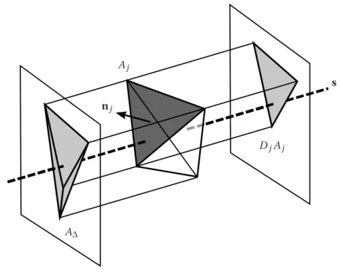
The diffusion term (a∇.∇∇∇Tn) can be solved using two methods. The first is derived from the cell-vertex discretization where a stencil of size 4∆ is used: the construction of the diffusion operator at one node requires the knowledge of the information of the two neighboring layers of cells (and nodes) as shown in Fig. 4.1-a. The second formulation is derived from a finite-element method with a vertex-centered discretization [101] that uses a smaller stencil of size 2∆: to construct the diffusion operator this method only needs the information of the closest layer of cells and nodes (Fig. 4.1-b). Details on the diffusion operators used in AVTP are presented by Lamarque [143].
(a) Cell-vertex discretization (b) Vertex-centered discretization Figure 4.1: Nodes and cells used in the computation of the diffusion operator on the central node. Four types of boundary conditions are available in AVTP:
8 Chapter 4: Heat transfer in solids
1. Isothermal wall (Dirichelt B.C.): the temperature of the boundary surfaces are imposed. 2. Heat loss wall (Neumann B.C.): the temperature evolution of the boundary surface depends
on the heat flux imposed through the knowledge of an external reference temperature Trefand
a covective heat transfer coefficient h.
3. Adiabatic wall (Neumann B.C.): is the same as the previous B.C. but the heat flux imposed is equal to zero.
4. Flux-Temperature wall (Mixed B.C.): mainly developed for coupled Fluid-Solit Thermal In-teraction (FSTI) applications, in this boundary condition a heat flux is imposed and a refer-ence temperature is added in order to help to code to converge to the target imposed: qs
w= qwre f+ k(T − Tref).
4.5
Analytical and numerical solutions for the transient heat equation
Textbooks on heat transfer cover the most basic methods for the resolution of the heat transfer equa-tion [152, 114, 110, 173, 251, 11], from the classical one-dimensional steady heat conducequa-tion problem to complex geometries like fins [152].
Among them, three resolution methods are discussed here and will be used as analytical references in four test cases to validate the simulations of the transient heat transfer problem. They are:
• Test case 1: the case of a small and highly conducting object plunged into a fluid at different temperature. The Low-Biot approximation is employed to determine its temperature evolution. • Test case 2: the computation of the temperature evolution on an one-dimensional externally heated solid slab subject to Dirichlet boundary conditions on both ends. The heat conduction equation is solved using the Fourier method.
• Test case 3: the computation of the temperature evolution on the same one-dimensional but this time cooled using Dirichlet boundary conditions on both ends. The Fourier method is also employed.
• Test case 4: the determination of the transient temperature of a solid wall subject to a Dirichlet boundary condition in one end and a Neumann boundary condition in the other. The Laplace
4.5 Analytical and numerical solutions for the transient heat equation 9
4.5.1
The Low-Biot approximation
Analytic solutionWhen the internal or external conditions of an originally stable medium are abruptly modified the system has to transit to a new stable state to achieve energy equilibrium. The time-evolution of the temperature in the solid is characterized by the Biot number Bi , which is proportional to the ratio between the convective heat transfer between the solid and the external flow and the conductive heat transfer within the solid:
Bi =hL
λ (4.19)
where L is a characteristic length scale of the solid.
If Bi ≪ 1 the main heat transfer process is conduction (low resistance of the solid). For a small and highly conductive sphere plunged into a fluid at different temperature (Bi ≪ 1), it has been shown that the temperature of the sphere evolves following expression (4.20) [152].
T −Text T0− Text= exp µ −ρCVhS t ¶ (4.20) where t is the time, Text is the temperature of the external flow, T0is the initial temperature of the
solid, S is the surface and V is the total volume of the solid. This analytical solution is the simplest version of the transient heat conduction equation. Diffusion of heat inside the solid is very fast. This analytical solution can be used to test the temporal integration of a heat conduction code and the reliability of the diffusion operator.
Furthermore, in real aeronautical applications this approximation can be useful to study the unsteady nature of the heat conduction, particularly in the thin layers of the combustion chamber liner and the walls of cane injectors.
Numerical simulation: test case 1
A benchmark case has been carried up in order to test AVTP under the Low-Biot approximation. In this case a 2D square of side length L = 0.001 [m], initially at the temperature T (t = 0) = T0= 400K, is
plunged into a fluid which is at a higher temperature Text= 600K. The total surface of the solid is given by S = 4L, and the volume1V = L ×L = 110−6[m2]. Given the heat conduction coefficient h = 100 [W
m−2 K−1], the density of the solid2 ρ= 7900 [kg m−3], the conductivity λ = 68.203929 [W m−1K−1]
and the heat capacity C = 450 [J K−1kg−1], the solution of eq.(4.20) can be written and is plotted in Fig. 4.2.
1Here the volume of the 2D solid must be considered equal to the area of the square. 2The properties of the solid presented in this paragraph correspond to the properties of iron.
10 Chapter 4: Heat transfer in solids 400 450 500 550 600 0 5 10 15 20 25 30 35 40 45 Te m p er at u re ,T [K ] time, [s] 400 450 500 550 600 0 5 10 15 20 25 30 35 40 45 Te m p er at u re ,T [K ] time, [s] AVTP Analytic
Figure 4.2: Temporal evolution of the solid temperature of test case 1.
In this case the Biot number is equal to Bi = 0.0001466 ≪ 1, and the highly conducting solid approx-imation can be applied. The characteristic conductive time is equal to τcond= L2/a ≈ 4.335 10−2 [s].
This characteristic time has an order of magnitude comparable with the characteristic times of some LES applications.
The simulation was carried out using a 30 x 30 cell mesh, and a convective flux boundary condition at all four limiting surfaces. The time evolution of the solid temperature is also plotted in Fig. 4.2 (sym-bols). The time step of such a simulation depends on the Fourier condition presented in eq.(4.18). In the present case this condition imposes a time step of ∆t = 2.8957 10−5[s]. This small time step is
comparable to the time steps observed the simulation of compressible flows using implicit numerical schemes.
4.5.2
Resolution by the Fourier method
Analytic solutionSimulations of quasi-1D wall offer a more complete benchmark case for heat conduction codes. Fig. 4.3 shows the studied geometry. It is a simple slab at an initial uniform temperature T0. A sudden
change of the temperature of the surfaces (Ts
w= 0) modifies the temperature field inside the slab in
space and time. The corresponding heat conduction equation writes:
∂2T ∂x2 = 1 a ∂T ∂t (4.21)
4.5 Analytical and numerical solutions for the transient heat equation 11 Initial condition: T (x, t = 0) = T0 Boundary conditions: ½ T (x = 0, t > 0) = Tws = 0 T (x = L, t > 0) = Tws = 0 L Tws Tws T0
Figure 4.3: Quasi one-dimensional slab. Test case 2.
The simplest way to solve the problem is using Fourier’s method: the temperature field is searched in the form of a linear combination of independent orthogonal functions: T (x, t) =P∞k=0Fk(x)Gk(t),
where Fk(x) and Gk(t) are functions that depend only on the space and the time variable respectively.
The functions depending only on one variable, the prime represents one differentiation of the func-tion with respect of that variable, i.e. F′
k= dFk/d x, G′k= dGk/d t, Fk′′= d2Fk/d x2and Gk′′= d2Gk/d t2.
Replacing T with this linear combination, each elementary solution Fk(x)Gk(t) must verify:
Fk(x)dGk(t)
d t = aGk(t) d2F (x)
d x2 (4.22)
which can be written:
G′ k Gk = a FkF ′′ k (4.23)
The Left-Hand Side (LHS) and the Right-Hand Side (RHS) of this equation are functions of different independent variables. This happens only when both sides are equal to a constant:
G′ k Gk = a Fk Fk′′= −mk (4.24)
Integrating eq.(4.24) for the function Gkgives:
G′k = −mkGk (4.25)
12 Chapter 4: Heat transfer in solids
In a similar way integrating eq.(4.24) for Fkgives: d2Fk d x2 = −mk a Fk (4.27) Fk(x) = K1cos³pmk/a x ´ + K2sin³pmk/a x ´ (4.28) Eq. (4.28) represents an infinite number of solutions of the differential system where K1and K2are
integration constants. From the boundary conditions the particular solution of the heat conduction problem presented in this section can be deduced:
x = 0 → K1= 0
x = L → sin(pmk/a L) = 0
where the second condition impliespmk/a L = kπ.
The full solution to the heat conduction equation is then:
T (x, t) =X∞ k
Bksin(kπx/L)exp(−k2t/τ) (4.29)
The orthogonality property of Fk, leads to the following expression for Bk:
Bk= RL 0 T0sin(kπx/L)d x RL 0 sin2(kπx/L)d x (4.30) which is equal to zero for pair values of k and gives Bk= 4T0/πk for odd values of k. We finally get:
T (x, t) =4T0 π
½
sin(πx/L)exp(−t/τ)+13sin(3πx/L)exp(−9t/τ)+15sin(5πx/L)exp(−25t/τ)+... ¾ (4.31) Eq. (4.31) represents the spatial and temporal evolution of a 1D slab that cools down from an initial temperature to zero. For an arbitrary boundary temperature Tws, expression (4.31) can be generalized, giving: T (x, t) = Txs− 4(T0− Tws) π ∞ X k 1 2k +1sin µ(2k +1)πx H ¶ exp µ−(2k + 1)t τ ¶ (4.32)
Numerical solution: the heating wall - test case 2
In this second test case, a 2D solid of length L is considered, with an infinite transverse size so that the thermal problem is can be considered one-dimensional. A uniform temperature of T0= 300K is

![Figure 4.7: Evolution of the temperature profile test case 3. The profiles correspond to times t = 100, t = 200, t = 400, t = 800, t = 1600, t = 3200, t = 6400, t = 12800, t = 25600 [s]](https://thumb-eu.123doks.com/thumbv2/123doknet/3715529.110804/46.892.227.627.198.496/figure-evolution-temperature-profile-test-profiles-correspond-times.webp)
![Figure 4.9: Spatial temperature profiles for seven different times (units, seconds [s]): (a) t = 1000, (b) t = 2000, (c) t = 4000, (d) t = 8000, (e) t = 16000, (f) t = 32000, (g) t = 64000](https://thumb-eu.123doks.com/thumbv2/123doknet/3715529.110804/48.892.231.628.196.495/figure-spatial-temperature-profiles-seven-different-times-seconds.webp)