Using Continuous Glucose Monitoring Data and Detrended
Fluctuation Analysis to Determine Patient Condition: A
Review
Felicity THOMAS1, Matthew SIGNAL2, and J Geoffrey CHASE2
1
BE (Hons), Department of Mechanical Engineering, University of Canterbury, New Zealand
2
PhD, Department of Mechanical Engineering, University of Canterbury, New Zealand
Work performed at:
- Department of Mechanical Engineering, University of Canterbury
Corresponding author: Prof J. Geoffrey Chase,
Department of Mechanical Engineering University of Canterbury,
Private Bag 4800 Christchurch New Zealand
Email: geoff.chase@canterbury.ac.nz
Financial Support: UC Department of Mechanical Engineering, New Zealand, Disclosures: None
Acknowledgements: None
Keywords: Continuous glucose monitoring, CGM, detrended fluctuation, DFA, fractal, review, sensor, diabetes, critical care, ICU
Figures and Table Count: 5 Figures main body 4 Figures Appendix 0 Tables
Abbreviations: Continuous glucose monitoring (CGM), Detrended Fluctuation Analysis (DFA), Multifractal Detrended Fluctuation Analysis (MFDFA), Blood Glucose (BG), Intensive Care Unit (ICU)
Abstract
Patients admitted to critical care often experience dysglycaemia and high levels of insulin resistance, various intensive insulin therapy protocols and methods have attempted to safely normalise blood glucose (BG) levels. Continuous glucose monitoring (CGM) devices allow glycaemic dynamics to be captured much more frequently (every 2-5mins) than traditional measures of blood glucose and have begun to be used in critical care patients and neonates to help monitor dysglycaemia. In an attempt to obtain a better insight relating biomedical signals and patient status, some researchers have turned towards advanced time series analysis methods.
In particular, Detrended Fluctuation Analysis (DFA) has been a topic of many recent studies in to glycaemic dynamics. DFA investigates the “complexity” of a signal, how one point in time changes relative to its neighbouring points, and DFA has been applied to signals like the inter-beat-interval of human heartbeat to differentiate healthy and pathological conditions.
Analysing the glucose metabolic system with such signal processing tools as DFA has been enabled by the emergence of high quality CGM devices. However, there are several inconsistencies within the published work applying DFA to CGM signals. Therefore, this paper presents a review and a “how to” tutorial of DFA, and in particular its application to CGM signals to ensure the methods used to determine complexity are used correctly and so that any relationship between complexity and patient outcome is robust.
Introduction
Patients admitted to critical care often experience dysglycaemia and high levels of insulin resistance [1-7]. Hence, various intensive insulin therapy protocols and methods have attempted to safely normalise blood glucose (BG) levels in critical care patients. These studies achieved a range of positive and negative results with the most successful showing a correlation between lower blood glucose and improved patient outcomes [1-3, 8-12]. However, negative results [13, 14] and difficulty with increased nurse workload [15-17] have led to the idea that continuous glucose monitoring (CGM) devices might be a necessary tool to obtain better BG control and safety.
In 2004 the first commercially available continuous glucose monitoring (CGM) device was released with FDA approval. CGM devices allow glycaemic dynamics to be captured much more frequently (every 2-5mins) than traditional measures of blood glucose. More recently, they have begun to be used in critical care patients and neonates to help monitor and monitor dysglycaemia [18-24].
In an attempt to obtain a better insight into biomedical signals researchers have turned towards advanced time series analysis methods. In particular, Detrended Fluctuation Analysis (DFA) has been a topic of many recent studies into glycaemic dynamics [19, 25-27]. DFA investigates the “complexity” of a signal, how one point in time changes relative to its neighbouring points. In the simplest of terms DFA characterises the variability or “fuzziness” of a signal. DFA has been applied to inter-breath-interval of human respiration, inter-beat-inter-breath-interval of human heartbeat and inter-stride-inter-breath-interval of human stride to differentiate between healthy and pathological conditions [28-34]. However, DFA requires a large, densely measured time series, limiting the signals it is applied to. Thus, analysing the glucose metabolic system with such signal processing tools as DFA is enabled by the emergence of high quality CGM devices that allow researchers to investigate if glucose complexity can be related to mortality [19, 25] or other outcomes.
This paper presents a “how to” tutorial and review of work applying detrended fluctuation analysis to CGM signals. From the current published literature applying DFA to CGM signals it is evident that before any conclusions can be drawn regarding the relationships between glucose complexity and mortality, the methods used to determine complexity must be used correctly and robustly. That requirement necessitates a clear, consistent understanding of the methods and their applications. Prior works and tutorials on DFA are highly mathematical and some aspects of DFA have evolved over time. Thus the methods are not necessarily easily accessible to many outside these mathematical fields. Thus, this article seeks to bridge that accessibility gap.
In particular this paper first introduces the terms, complexity, self-similarity, monofractal and multifractal. The paper then discusses how to determine if a signal is of the correct form for mono or multifractal analysis and the meaning of what each analysis produces. It also addresses the considerations needed for the correct implementation for DFA to be undertaken. Applications to CGM data from critical care patients are highlighted for clinical context and to demonstrate these concepts.
What is Complexity, Self-similarity, Monofractal and Multifractal?
The complexity of a signal is how one point in a time series relates to the next or the previous point in a time series. A signal with high complexity will have many rapid changes between neighbouring points, as shown in Figure 1 panel A, while a signal with low complexity will not, Figure 1 panel B. This complexity can be defined using monofractal DFA which defines complexity as one unit-less number, the Hurst co-efficient (H) or multifractal DFA which defines complexity as a multifractal spectrum, Panels C and D. Which analysis, monofractal or multifractal, is appropriate for the signal depends on if the signal is mono or multifractal in structure.
Figure 1: A comparison of a signal with low complexity (panel A)) and a signal with high complexity (panel B). The monofractal DFA was used to produce a Hurst coefficient for each signal, 1.23 and 1.83, respectively. Multifractal DFA was used to determine the multifractal spectrum for each signal, panel C and D, respectively. The width of this spectrum can also be used to define the complexity of each signal as was calculated as 1.09 and 1.39 respectively.
If the signal is monofractal in structure it will be self-similar and this self-similarity will not change as time and space change [33, 35-37]. To be self-similar a signal must repeat it’s self on multiple scales. To visualise this repetition, think of a fern leaf, if you look closer at the fern leaf you will be able to see
0 2000 4000 6000 8000 4 6 8 Time M a g n it u d e
Signal with Low Complexity - H = 1.23
0 2000 4000 6000 8000 4 6 8 Time M a g n it u d e
Signal with High Complexity - H = 1.82
0.5 1 1.5 2 2.5 3 0 0.5 1 h(q) D (q )
Multifractal Spectrum - Width = 1.09
0.5 1 1.5 2 2.5 3 0 0.5 1 h(q) D (q )
Multifractal Spectrum - Width = 1.39
A
D C
many small fern leafs inside the big fern leaf and many fern leafs inside of these smaller fern leafs and so on and so forth. This is a self-similar or fractal structure. To undertake any type of detrended fluctuation analysis this self-similar structure must be apparent. If the signal is multifractal the signal will be self-similar but this will change as time and space changes and the complexity of the signal can no longer be defined by H it must be defined by the multifractal spectrum.
There is no way to tell from just looking at a signal if it is self-similar, monofractal or multifractal. The step by step process to ensuring that a signal is self-similar and determining if a signal is multifractal or monofractal is outlined in the following section, DFA implementation. The section is followed by an analysis of the literature using DFA and results in a list of the key steps and requirements for using DFA correctly to ensure good results.
Finally, for the purpose of this review, it should be noted that not every reader needs to be able to apply DFA to a signal or understand every equation in this paper. However, if they can understand the required signal characteristics and key steps to perform DFA correctly, then they will be in a far better place to interpret and evaluate DFA results or analyses in the literature.
DFA Implementation
This section outlines the methods used by many different authors to carry out detrended fluctuation analysis for mono and multifractal biomedical signals. First, the key steps required to perform DFA, are summarised in Figure 2 and a step by step example implementing these key steps can be found in the supplementary file. It is important to note that DFA methods for biomedical signals has evolved
Fractal Analysis cannot be under taken
Step 1
Is the signal
self-similar? No
Step 2
Is the signal Monofractal or Multifractal?
Step 4b
The mulitfractal
spectrum defines the
complexity of the signal
Step 4a
The complexity of the signal can be defined
by the Hurst coefficient Step 3a Is the signal > 500 measurements? Step 3b Is the signal > 1000 measurements? The signal is not long enough for fractal analysis The signal is not long enough for fractal analysis Yes Yes Yes Monofractal No No Multifractal
Figure 2: Flow Chart of the process required to implement detrended fluctuation analysis. A step by step example is contained in the supplementary file, implementing these steps for a CGM signal.
since it was first applied by Peng et al in 1994 [38]. Therefore, this section aims to highlight all the approaches that have been published to date to give insight and indicate the work necessary for DFA to become a trusted signal processing tool for CGM signals.
Step 1 – Is the signal self-similar?
When Peng et al [39] first introduced the concept of DFA to the biomedical field it was applied to easily and clearly measureable heartbeat time series where very large numbers of data points can be easily obtained. The authors then further detail the method in a separate journal article using a random walk describing the organisation of DNA nucleotides [38]. Importantly, both these signals display long range power-law correlations that indicate self-similarity across a number of decades of data [38, 39], which means the signal is exactly or approximately similar to a part of itself on many different time scales. To ensure fractal analysis can be carried out on a CGM signal three features of self-similarity must be evident [40]:
1. At a scale 1/r when rescaled by rH X(rt) the signal looks the same as the original X(t) and is
statistically indistinguishable from it.
2. Fourier power spectrum of the signal - if the frequency is doubled the power diminishes by the same fraction regardless of frequency
3. Autocorrelation: Gaussian signals will show correlated or anti-correlated structuring, while in Brownian motion signals have neighbouring elements that are positively correlated. The equations for the correlation and correlation coefficients are thoroughly described in Eke et al. [40].
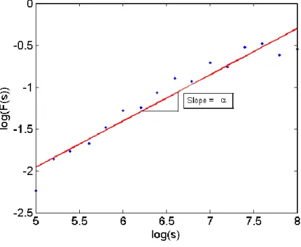
However, the simplest way to check the self-similarity of a signal is to plot log (F(𝑠)) versus log(s) [35], as defined:
𝑌(𝑖) = ∑𝑖𝑘=1[𝑥𝑘− 〈𝑥〉], 𝑖 = 1, … , 𝑁 Equation 1
Where F(s) is the root mean square (RMS) of the variance between the time series, x, and the least squares fit for each segment, ys(i), and s is the segment sample size. If this plot displays a linear
relationship the signal is self-similar [35], as shown in Figure 3. Self-similarity needs to be apparent over at least two decades of frequency before confidence in using fractal approaches can be assured [40].
Figure 3: The overall RMS F(s) plotted against s the segment sample size. The linear relationship over at least two decades (3 decades in this case) deems fractal analysis appropriate for this signal.
Step 2 – Is the signal Monofractal or Multifractal?
For Monofractal DFA to be valid the signal must have self-similarity that is independent of time or space [33, 35-37]. This means the Hurst coefficient must remain constant across all q-order statistical moments [35, 37]. More simply, the signal must be simple enough to be described by one fractal dimension. When the self-similarity of a time series changes with spatial and temporal variations, the signal is deemed to be multifractal [35].
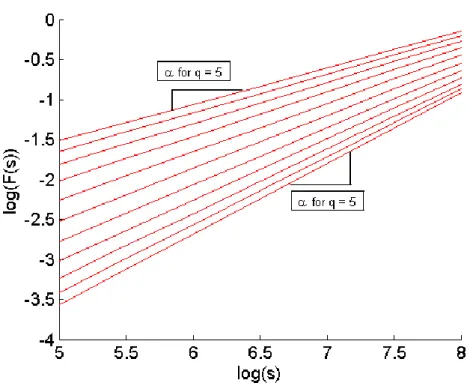
To determine if the self-similarity of a signal dependent on time and space we can plot the relationship of log(Fq(s)) versus log (s) and if the slope this this relationship changes with q-order statistical
moments [35] as shown in Figure 4 and given by: 𝐹2(𝑣, 𝑠) =1 𝑠∑ (𝑌[(𝑣 − 1)𝑠 + 𝑖] − 𝑦𝑣(𝑖)) 2 𝑠 𝑖=1 Equation 3 𝐹𝑞(𝑠) = { 1 𝑁𝑠∑ [𝐹 2(𝑣, 𝑠)]𝑞⁄2 𝑁𝑠 𝑣=1 } 1 𝑞 ⁄ Equation 4
When q = 0 a logarithmic averaging proceedure must be employed instead of Equation 4: 𝐹0(𝑠) = 𝑒𝑥𝑝 { 1 2𝑁𝑠∑ log[𝐹 2(𝑣, 𝑠)] 𝑁𝑠 𝑣=1 } Equation 5
Figure 4: An Example log(Fq(s)) versus log(s) plot. Note the linear relationship changes with q order statistical moments hence multifractal analysis is appropriate for this signal
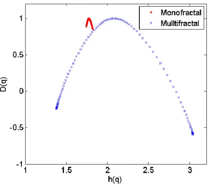
If unsure, it is wise to also plot the multifractal spectrum as it will clearly show if the signal is multi or monofractal, as shown in Figure 5, where the spectrum for a monofractal signal will be very narrow. The equations to generate the multifractal spectrum are defined:
𝜏(𝑞) = 𝑞. 𝐻(𝑞) − 1 Equation 6
ℎ(𝑞) = 𝜏′(𝑞) Equation 7
𝐷(𝑞) = 𝑞. ℎ(𝑞) − 𝜏(𝑞) Equation 8
Where q is the statistical moment and H(q) is the Hurst coefficient for that statistical moment. A plot of 𝐷(𝑞) vs. ℎ(𝑞) displays the mulitfractal spectrum.
Figure 5: Example of multifractal spectrum that is produced from multifractal DFA. Note the monofractal signal produces a very narrow spectrum, indicating monofractal scaling is present and monofractal DFA is sufficient to characterise the scaling and correlation properties of the signal
Step 3a and 3b – Signal length
For the results of mono or multifractal DFA to be valid the signals must be of appropriate minimum length [33, 36, 40-43]. For monofractal DFA it is recommended that the signal be greater than 512
points long for results with a bias and standard deviation of less than 0.05 [43]. However, to have a 0.95 probability of distinguishing between two signals with true Hurst coefficient differing by 0.1, more than 32768 points are required [43]. This number of points is feasible for a biological signal like heart beats, but is more difficult for CGM with typically 288 measurements a day. For Multifractal DFA results from signals less than 1000 measurements are to be viewed with caution [35]. The larger the sample size the larger the range of segment sizes to allowing both fast and slow fluctuations to be captured [35].
In comparison to the well-known Fast Fourier Transform (FFT), the signal length has similar implications. The FFT is a very common signal analysis tool using similarly long signals that provides a structured sum of sine wave terms to capture the shape of an arbitrary, assumed periodic signal. The length of data points used thus defines the resolution and accuracy of that decomposition from a general signal to a sum of sine waves at different frequencies.
In contrast, DFA provides an arbitrary capture of a general signal as calculated from Equation (2), or Equations (3-5) for multifractal analysis, based on RMS variability from point to point, which is quite different than the structured sum of sine waves in a FFT. For DFA, as with the FFT, the length of the signal determines the level of resolution and accuracy. However, given their entirely different formulation, there is no direct analogy from FFT analysis of frequency content to the DFA analysis of point to point variability and complexity.
Step 4a – Calculating the Hurst Coefficient
When Peng et al first used DFA in 1993 [39] they were not concerned with calculating the Hurst coefficient. They only aimed to prove the F(s) α sα power-law relationship existed for the scale
invariant heart beat time series and how the value of α could appear markedly different for pathological and healthy conditions [39]. However, the signal type and resulting methods used vary between the first three publications from Peng et al on DFA [32, 38, 39]. Eke et al in 2002 [33] produced an overview of fractal complexity analysis. A more generic method for DFA was included in this paper, referencing Peng et al [38], which allows both Gaussian and Brownian type signals to be analysed and a Hurst coefficient obtained. The main computational steps for a successful DFA and calculation of the Hurst coefficient are:
1. Integrate time series by summing and subtracting the mean creating a zero centred signal 𝑌(𝑖) = ∑𝑖𝑘=1[𝑥𝑘− 〈𝑥〉], 𝑖 = 1, … , 𝑁 Equation 1
2. Choose sample size, s, and divide profile into Ns non-overlapping segments of equal length s
3. Determine the trend for each segment, the root mean square (RMS) of the variance between the time series, x, and the least squares fit for each segment, ys(i)
𝐹(𝑠) = √1
𝑠∑ (𝑌(𝑖) − 𝑦𝑠(𝑖)) 2 𝑠
𝑖=1 Equation 2
4. Repeat Steps 2 and 3 for a range of segment sizes, s. Note that fast fluctuations in the series will influence F for segments with small sample sizes, whereas slow changing fluctuations will influence F for segments with larger sample sizes. Hence multiple scales necessary to capture both fast and slow fluctuations [35]. A rule of thumb for the number of segment sizes needed is >5 segments between 10 and N/2 [36].
5. Plot F(s) vs. s and calculate the slope of the line, α 6. Relate α to the Hurst coefficient
a. if α < 1 then the signal is Gaussian α = H b. if α > 1 then the signal is Brownian α = H + 1
To implement these steps, Ihlen [35] produced a self-sustained guide with downloadable Matlab files [35].
While [35] is mainly focused on multifractal DFA the code for monofractal DFA is included and explained. It is important to remember that DFA is not the only fractal analysis that characterises the complexity of a signal using the Hurst coefficient. There are many other ways of calculating H including scaled window variance methods, rescaled range analysis, dispersional analysis and maximum likelihood estimation [33, 36]. These analyses may produce a more accurate estimation of the Hurst coefficient for specific types of signals. A summary of the benefits and drawbacks of these different type of fractal analysis has been produced by Delignieres et al [36].
Step 4b – Producing the Multifractal spectrum
When the self-similarity of a time series changes with spatial and temporal variations, the signal is deemed to be multifractal [35], as described in Section 1, Step 2 and Figure 4. The complexity of such a sign is defined by a multifractal spectrum of power law exponents [35]. Kantelhardt et al [44] developed multifractal detrended fluctuation analysis (MFDFA) in 2002. The method to successfully implement MFDFA are well outlined in clear steps in this paper and have not evolved over time as they have for monofractal DFA. Readers are referred to [44] as a first step in understanding and undertaking MFDFA analysis.
Some of the potential pitfalls in MFDFA include large errors induced in the multifractal spectrum if the RMS is close to zero as log(F) becomes infinitely small [35]. This issue can be resolved by eliminating RMS below a certain threshold, such as the precision of the measurement device that is recording the biomedical time series. Another issue is being able to distinguish if the signal being analysed is a random walk or noise like signal, and, therefore, if the signal requires transformation to a noise like signal before analysis. Eke et al [33] suggest first applying monofractal DFA to the signal and if the Hurst coefficient is between 0.2-1.2 the signal is a noise like signal and does not require transformation. However, if the signal is between 1.2-1.8 the signal is a random walk and needs to be
differentiated before undertaking MFDFA. As mentioned previously in Step 1, it is also imperative to ensure the time series is self-similar.
It is important to remember that MFDFA is not the only way of producing the multifractal spectrum to analyse the complexity of a signal. For example, there are multifractal analyses based on wavelet transforms, the results of which can be compared directly to MFDFA [28, 35, 45]. Performance of MFDFA has been shown to be comparable to the wavelet transform methods, unless the time series contains strong oscillatory or ramp like trends, where wavelet transform methods are preferred [35, 45]. Hence, MFDFA is the main focus of this tutorial.
The width, shape and location of the mulifractal spectrum can all be used to define the complexity of the time series being studied [35]. Differences in these variables between certain cohorts can be used to investigate relationships between the time series and the physiological phenomenon being studied. Elements of the mutlifractal spectrum have been used successfully to differentiate between certain heart diseases and the neural activity of different brain areas [46-48]. Therefore it is plausible to suggest that CGM signals could produce some indicator of mortality or significant metabolic or organ dysfunction from the differences in multifractal spectrum. However, the results from an initial investigation by Signal et al could not find a relationship between the multifactal spectrum and patient outcome [49].
DFA, CGM and the ICU – Clinical Implementation
The first study to investigate glucose complexity in critical care patients was Lundelin et al in 2010 [25]. Monofractal DFA was applied to a cohort of 38 patients each with 1 CGM signal during a 24 hour period (n = 288 measurements). In this study Lundelin et al found mean Hurst coefficients of 1.49 and 1.60 for survivors and non survivors, respectively (P=0.015). Thus, Lundelin et al concluded that loss of complexity in a glycaemic time series, evaluated by DFA, correlates with higher mortality in the
critically ill. However, the authors do not mention if the fractility of the signal was checked or questioned. In addition, to ensure the results of any monofractal DFA analysis are reliable with a bias and standard deviation of less than 0.05, the number of samples must be greater than 512 [41]. Any series with n < 258 cannot be considered reliable [41]. Each CGM trace analysed in Lundelin et al has only n = 288 measurements. Thus, the shortness of the time series used may significantly impact the conclusions drawn.
In a follow up study to Lundelin et al, Brunner et al [19] applied monofractal DFA to a larger cohort of 174 patients, with a larger time series of n= 710 for each patient. They found a mean Hurst coefficient for survivors of 1.52, which was lower than the mean coefficient for non-survivors of 1.61 (p = 0.01), matching the results in Lundelin et al. From these results they drew the same conclusion that loss of complexity in glycaemia time series, evaluated by DFA, correlates with higher mortality.
However, as in [25] the authors of [19] do not mention if they investigated the fracticality of the CGM signals to ensure they were monofractal. Hence, it is not possible to conclude if monofractal DFA analysis is appropriate for this data set. In addition, in this study, there is a mix of CGMS gold retrospective devices (Medtronic Minimed, Northridge, CA, USA) and newer Guardian CGMS real time devices (Medtronic Minimed, Northridge, CA, USA). The calibration and signal processing for retrospective and real time devices is very different, where real time devices generally have a much higher noise content as they only have previous calibration values to guide blood glucose estimation. In contrast, retrospective devices fit a profile through all calibration measurements and “know” the future values at any point. This difference can lead to vastly different signals being produced by each device [50]. For example, Signal et al [49] found the Hurst coefficient varied more between retrospective and real time devices, than between survivors and non survivors.
This third study of glucose complexity in the critically ill, by Signal et al [49] did test the fractal structure of the CGM signals with n > 500. It found that the CGM traces used for this analysis had a multifractal composition. Thus, monofractal DFA was not deemed an appropriate method to characterise the complexity of these signals. In contrast, multifractal analysis produces a spectrum of Hurst coefficients. Signal et al compared these spectrums, but found no association between complexity and mortality.
Patients admitted to ICU are highly variable and can have a range of conditions or treatments that may impact on the accuracy of CGM, such as oedema, sepsis, cooling blankets and pressure around the sensor site [51, 52]. All of these factors affect sensor performance and will subsequently affect the results obtained from DFA. Also while inserting the CGM sensor in the subcutaneous layer is minimally invasive and generally safe from infection it can introduce increased noise and error within the output [21, 53-56]. Similarly, calibration differences or device sensor differences will change the glucose trace and the DFA results. It is important that any persons wanting to undertake DFA on CGM data from ICU patients, or other subjects, are aware of these potential confounding issues.
Signal et al. [49] produced an interesting example of the potential effect of sensor performance on DFA results. A patient had three identical sensors inserted, all of which appeared to agree and track a similar glucose profile. However, the Hurst co-efficient and multifractal spectrum produced by each trace was markedly different. The authors also included an example where a patient had two identical sensors inserted, which did not show similarity in their output trace, but produced almost identical Hurst coefficients and multifractal spectrums.
With these issues in mind, the authors have generated a list of clinical factors that should be considered for a study using DFA to assess the complexity of ICU patients CGM signals.
1) Consistency of device type and calibration method [49] 2) Consistency of sensor insertion location on the body
3) Avoiding highly oedematous or septic patients as effects of such conditions are still under investigation or at least recording an “oedema score” so that like patients can be compared 4) Diligence in recording medications and treatments that could affect sensor performance
Conclusion
This paper presents a step by step tutorial and review of detrended fluctuation analysis for use with continuous glucose monitoring signals from intensive care patients. From this review it is clear that before any conclusions can be drawn regarding the relationships between glucose complexity and mortality the methods used to determine complexity must be used correctly and robustly. In particular regarding the mathematical analysis of the data it is important the form of the data either, mono or multifractal, is considered to select the right analysis for the data. It is also imperative that the signal lengths are long enough to ensure reliable results. Furthermore for the correct clinical implementation consistent sensor type and location should be applied. Also important that users are consider and report the clinical factors which could impact the CGM signals and therefore DFA results such as medication and patient condition.
References
1. Capes, S.E., et al., Stress hyperglycaemia and increased risk of death after myocardial
infarction in patients with and without diabetes: a systematic overview. Lancet, 2000. 355(9206): p. 773-778.
2. Finney, S.J., et al., Glucose control and mortality in critically ill patients. Jama, 2003. 290(15): p. 2041-2047.
3. Krinsley, J.S., Association between hyperglycemia and increased hospital mortality in a
heterogeneous population of critically ill patients. Mayo Clin Proc, 2003. 78(12): p.
1471-1478.
4. Mizock, B.A., Alterations in fuel metabolism in critical illness: hyperglycaemia. Best Pract Res Clin Endocrinol Metab, 2001. 15(4): p. 533-51.
5. McCowen, K.C., A. Malhotra, and B.R. Bistrian, Stress-induced hyperglycemia. Crit Care Clin, 2001. 17(1): p. 107-124.
6. Umpierrez, G.E., et al., Hyperglycemia: an independent marker of in-hospital mortality in
patients with undiagnosed diabetes. J Clin Endocrinol Metab, 2002. 87(3): p. 978-982.
7. Van den Berghe, G., et al., Outcome benefit of intensive insulin therapy in the critically ill:
Insulin dose versus glycemic control. Crit Care Med, 2003. 31(2): p. 359-366.
8. Bistrian, B.R., Hyperglycemia and Infection: Which is the Chicken and Which is the Egg? JPEN J Parenter Enteral Nutr, 2001. 25(4): p. 180-181.
9. Van den Berghe, G., et al., Intensive insulin therapy in the critically ill patients. N Engl J Med, 2001. 345(19): p. 1359-1367.
10. Krinsley, J.S., Effect of an intensive glucose management protocol on the mortality of
critically ill adult patients. Mayo Clin Proc, 2004. 79(8): p. 992-1000.
11. Chase, J.G., et al., Implementation and evaluation of the SPRINT protocol for tight glycaemic
control in critically ill patients: a clinical practice change. Critical Care, 2008. 12(2): p. R49.
12. Signal, M., et al., Glycemic levels in critically ill patients: are normoglycemia and low
variability associated with improved outcomes? J Diabetes Sci Technol, 2012. 6(5): p. 1030-7.
13. Finfer, S., et al., Intensive versus conventional glucose control in critically ill patients. N Engl J Med, 2009. 360(13): p. 1283-97.
14. Brunkhorst, F.M., et al., Intensive insulin therapy and pentastarch resuscitation in severe
sepsis. N Engl J Med, 2008. 358(2): p. 125-39.
15. Carayon, P. and A. Gurses, A human factors engineering conceptual framework of nursing
workload and patient safety in intensive care units. Intensive Crit Care Nurs, 2005. 21(5): p.
284-301.
16. Holzinger, U., et al. ICU-staff education and implementation of an insulin therapy algorithm
improve blood glucose control. in 18th ESICM Annual Congress. 2005. Amsterdam,
Netherlands.
17. Mackenzie, I., et al., Tight glycaemic control: a survey of intensive care practice in large
English hospitals. Intensive Care Med, 2005. 31(8): p. 1136.
18. Chee, F., T. Fernando, and P.V. van Heerden, Closed-loop glucose control in critically ill
patients using continuous glucose monitoring system (CGMS) in real time. IEEE Trans Inf
Technol Biomed, 2003. 7(1): p. 43-53.
19. Brunner, R., et al., Glycemic variability and glucose complexity in critically ill patients: a
retrospective analysis of continuous glucose monitoring data. Crit Care, 2012. 16(5): p. R175.
20. Holzinger, U., et al., Real-time continuous glucose monitoring in critically ill patients: a
prospective randomized trial. Diabetes Care, 2010. 33(3): p. 467-72.
21. Rabiee, A., et al., Numerical and clinical accuracy of a continuous glucose monitoring system
during intravenous insulin therapy in the surgical and burn intensive care units. J Diabetes Sci
22. Signal, M., et al., Continuous glucose monitors and the burden of tight glycemic control in
critical care: can they cure the time cost? J Diabetes Sci Technol, 2010. 4(3): p. 625-35.
23. Beardsall, K., et al., The continuous glucose monitoring sensor in neonatal intensive care. Archives of Disease in Childhood, 2005. 90(4): p. F307-F310.
24. Harris, D.L., et al., Continuous Glucose Monitoring in Newborn Babies at Risk of
Hypoglycemia. Journal of Pediatrics, 2010. 157(2): p. 198-202.
25. Lundelin, K., et al., Differences in complexity of glycemic profile in survivors and nonsurvivors
in an intensive care unit: a pilot study. Crit Care Med, 2010. 38(3): p. 849-54.
26. Yamamoto, N., et al., Detrended fluctuation analysis is considered to be useful as a new
indicator for short-term glucose complexity. Diabetes Technol Ther, 2010. 12(10): p. 775-83.
27. Ogata, H., et al., Long-range negative correlation of glucose dynamics in humans and its
breakdown in diabetes mellitus. Am J Physiol Regul Integr Comp Physiol, 2006. 291(6): p.
R1638-43.
28. Wink, A.M., et al., Monofractal and multifractal dynamics of low frequency endogenous
brain oscillations in functional MRI. Hum Brain Mapp, 2008. 29(7): p. 791-801.
29. Hausdorff, J.M., Gait dynamics, fractals and falls: finding meaning in the stride-to-stride
fluctuations of human walking. Hum Mov Sci, 2007. 26(4): p. 555-89.
30. Lee, J.M., et al., Nonlinear-analysis of human sleep EEG using detrended fluctuation analysis. Med Eng Phys, 2004. 26(9): p. 773-6.
31. Peng, C.K., et al., Quantifying fractal dynamics of human respiration: age and gender effects. Ann Biomed Eng, 2002. 30(5): p. 683-92.
32. Peng, C.K., et al., Quantification of Scaling Exponents and Crossover Phenomena in
Nonstationary Heartbeat Time-Series. Chaos, 1995. 5(1): p. 82-87.
33. Eke, A., et al., Fractal characterization of complexity in temporal physiological signals. Physiol Meas, 2002. 23(1): p. R1-38.
34. Goldberger, A.L., et al., Fractal dynamics in physiology: alterations with disease and aging. Proc Natl Acad Sci U S A, 2002. 99 Suppl 1: p. 2466-72.
35. Ihlen, E.A., Introduction to multifractal detrended fluctuation analysis in matlab. Front Physiol, 2012. 3: p. 141.
36. Delignieres, D., et al., Fractal analyses for 'short' time series: A re-assessment of classical
methods. Journal of Mathematical Psychology, 2006. 50(6): p. 525-544.
37. Eke, A., et al., Pitfalls in Fractal Time Series Analysis: fMRI BOLD as an Exemplary Case. Front Physiol, 2012. 3: p. 417.
38. Peng, C.K., et al., Mosaic organization of DNA nucleotides. Phys Rev E Stat Phys Plasmas Fluids Relat Interdiscip Topics, 1994. 49(2): p. 1685-9.
39. Peng, C.K., et al., Long-Range Anticorrelations and Non-Gaussian Behavior of the Heartbeat. Physical Review Letters, 1993. 70(9): p. 1343-1346.
40. Eke, A., et al., Physiological time series: distinguishing fractal noises from motions. Pflugers Arch, 2000. 439(4): p. 403-15.
41. Bassingthwaighte, J.B. and G.M. Raymond, Evaluation of the dispersional analysis method for
fractal time series. Ann Biomed Eng, 1995. 23(4): p. 491-505.
42. Bassingthwaighte, J.B. and G.M. Raymond, Evaluating rescaled ranged analysis for time
series. Ann Biomed Eng, 1994. 22(4): p. 432-44.
43. Cannon, M.J., et al., Evaluating scaled windowed variance methods for estimating the Hurst
coefficient of time series. Physica A, 1997. 241(3-4): p. 606-626.
44. Kantelhardt, J.W., et al., Multifractal detrended fluctuation analysis of nonstationary time
series. Physica a-Statistical Mechanics and Its Applications, 2002. 316(1-4): p. 87-114.
45. Huang, Y.X., et al., Arbitrary-order Hilbert spectral analysis for time series possessing scaling
statistics: comparison study with detrended fluctuation analysis and wavelet leaders. Phys
46. Zheng, Y., et al., Multiplicative multifractal modeling and discrimination of human neuronal
activity. Physics Letters A, 2005. 344(2-4): p. 253-264.
47. Wang, G., et al., Multifractal analysis of ventricular fibrillation and ventricular tachycardia. Medical Engineering & Physics, 2007. 29(3): p. 375-379.
48. Ivanov, P.C., et al., Multifractality in human heartbeat dynamics. Nature, 1999. 399(6735): p. 461-465.
49. Signal, M., et al., Complexity of continuous glucose monitoring data in critically ill patients:
continuous glucose monitoring devices, sensor locations, and detrended fluctuation analysis methods. J Diabetes Sci Technol, 2013. 7(6): p. 1492-506.
50. Signal, M., Continuous Glucose Monitoring and Tight Glycaemic Control in Critically Ill
Patients in Bioengineering 2013, University of Canterbury University of Canterbury.
51. Lorencio, C., et al., Real-time continuous glucose monitoring in an intensive care unit: better
accuracy in patients with septic shock. Diabetes Technol Ther, 2012. 14(7): p. 568-75.
52. Moser, E.G., L.B. Crew, and S.K. Garg, Role of continuous glucose monitoring in diabetes
management. Avances en Diabetología, 2010. 26(2): p. 73-78.
53. Vlkova, A., et al., Blood and tissue glucose level in critically ill patients: a comparison of
different methods of measuring interstitial glucose levels. Intensive Care Med, 2009. 35(7): p.
1318.
54. Klonoff, D.C., A review of continuous glucose monitoring technology. Diabetes Technol Ther, 2005. 7(5): p. 770-5.
55. Klonoff, D.C., Continuous Glucose Monitoring: Roadmap for 21st century diabetes therapy. Diabetes Care, 2005. 28(5): p. 1231-9.
56. Castle, J.R. and W.K. Ward, Amperometric glucose sensors: sources of error and potential
Supplementary File: A Worked Example
The following example uses CGM data from an Ipro2 CGM device (Medtronic Minimed, Northridge, CA, USA) that was inserted into the abdomen of a healthy individual and worn for 6 days. Blood glucose was measured 4 times a day prior to meals and sleeping. These measurements were used to calibrate the device. Calibration BG measurements were taken using capillary finger stick measurements and the Abbott Optimum Xceed (Abbott Diabetes Care, Alameda, CA) glucometer.
Figure S1: CGM trace used for the worked example. Step 1 – Is the Signal Self Similar?
Using Equation 1 and 2 a of plot log (F(𝑠)) versus log(s) was generated. Where segment sizes, s = [32, 45, 64, 91, 128, 181, 256, 362, 512] were used to generate the non-overlapping segments of equal length, Ns required. The segment sizes where selected to allow both fast and slow fluctuations to be
captured but to be no longer that half the signal (N = 1715).
10003 2000 3000 4000 5000 6000 7000 8000 9000 3.5 4 4.5 5 5.5 6 6.5 7 7.5 8 Time (days) G lu c o s e ( m m o l/ L )
Figure S2: Plot of log (F(𝑠)) versus log(s)
As shown in Figure S2 the relationship between log (F(𝑠)) and log(s) is linear hence the signal is self-similar and therefore fractal analysis can be undertaken. The slope of the linear regression line, α, is 1.21 thus the signal is Brownian or a random walk signal and H = α +1,
Step 2 – Is the Signal multifractal or monofractal?
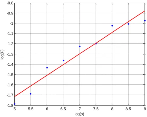
Using Equation 3, 4 and 5 values of (𝐹𝑞(𝑠)) were generated for integer values of q, -5 < q < 5. The slope
the (𝐹𝑞(𝑠)) for versus log (s) linear regression lines were calculated for each q, α(q). In Step 1 the signal
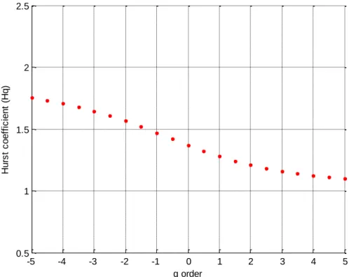
was found to be a random walk hence H(q) = α(q) + 1. Also the signal was not integrate before this process was undertaken, a process that a Gaussian noise signal would require. H(q) was then plotted against q. 5 5.5 6 6.5 7 7.5 8 8.5 9 -1.8 -1.7 -1.6 -1.5 -1.4 -1.3 -1.2 -1.1 -1 -0.9 -0.8 lo g (F ) log(s)
Figure S3: H(q) as a function of q order
This Figure S3 show how the linear relationship changes with q order statistical moments. Hence, multifractal analysis is appropriate for this signal
Step 3 – Is the Signal long enough?
For Multifractal signals the signal must be greater than 1000 data points for the results to be trust worth. This signal had N = 1715 so the signal length should not negatively impact the results.
Step 4 - Implementation of DFA
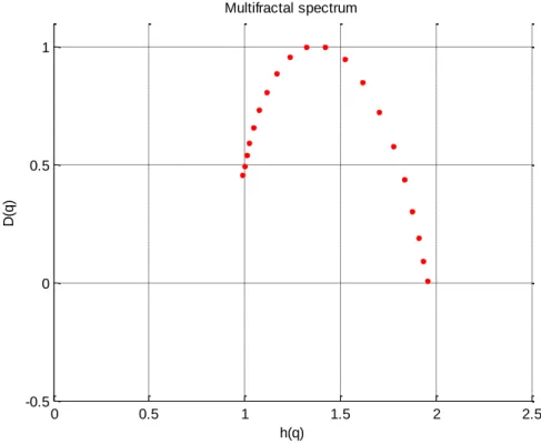
Equations 6, 7 and 8 were then employed to calculated D(q) and h(q) which when plotted against each other produce the multifractal spectrum.
-5 -4 -3 -2 -1 0 1 2 3 4 5 0.5 1 1.5 2 2.5 q order H u rs t c o e ff ic ie n t (H q )
Figure S4: The multifractal Spectrum of the CGM trace
The width of the spectrum is then calculated as h(q)max – h(q)min = 0.96.
0 0.5 1 1.5 2 2.5 -0.5 0 0.5 1 Multifractal spectrum h(q) D (q )