UNIVERSITF.DE
SHERBROOKE
Faculte de genie
Departement de genie civil
REPONSE DYNAMIQUE DES STRUCTURES SOUS
CHARGES DE VENT
These de doctorat es sciences appliquees
Speciality : genie civil
Ferawati GANI
Jury : Frederic LEGERON (Directeur)
Charles-Philippe LAMARCHE (Rapporteur)
Louis CLOUTIER
Pierre VAN DYKE
Hachimi FELLOUAH
Elena DRAGOMIRESCU
Sherbrooke (Quebec), Canada Avril 2011
Library and Archives Canada Published Heritage Branch 395 Wellington Street Ottawa ON K1A 0N4 Canada Bibiiotheque et Archives Canada Direction du Patrimoine de ['edition 395, rue Wellington Ottawa ON K1A 0N4 Canada
Your file Votre reference ISBN: 978-0-494-83325-4 Our file Notre reference ISBN: 978-0-494-83325-4
NOTICE:
The author has granted a
non-exclusive license allowing Library and Archives Canada to reproduce, publish, archive, preserve, conserve, communicate to the public by
telecommunication or on the Internet, loan, distrbute and sell theses
worldwide, for commercial or non-commercial purposes, in microform, paper, electronic and/or any other formats.
AVIS:
L'auteur a accorde une licence non exclusive permettant a la Bibiiotheque et Archives Canada de reproduire, publier, archiver, sauvegarder, conserver, transmettre au public par telecommunication ou par llnternet, preter, distribuer et vendre des theses partout dans le monde, a des fins commerciales ou autres, sur support microforme, papier, electronique et/ou autres formats.
The author retains copyright ownership and moral rights in this thesis. Neither the thesis nor substantial extracts from it may be printed or otherwise reproduced without the author's permission.
L'auteur conserve la propriete du droit d'auteur et des droits moraux qui protege cette these. Ni la these ni des extraits substantias de celle-ci ne doivent etre imprimes ou autrement
reproduits sans son autorisation.
In compliance with the Canadian Privacy Act some supporting forms may have been removed from this thesis.
While these forms may be included in the document page count, their removal does not represent any loss of content from the thesis.
Conformement a la loi canadienne sur la protection de la vie privee, quelques formulaires secondares ont ete enleves de cette these.
Bien que ces formulaires aient inclus dans la pagination, il n'y aura aucun contenu manquant.
R e s u m e
L'interet principal de cette recherche est d'assembler des outils numeriques afin de realiser, de far^on realiste, des analyses dynamiques de structures sous charges de vent. La dispo-nibilite de ces outils numeriques est devenue importante suite a des evenements de vents extremes ayant cause des dommages a plusieurs structures. La methodologie principale de cette etude est divisee en deux grandes parties : (i) preparer des charges de vent selon leurs correlations spatiales et temporelles en utilisant le vent genere de facon numerique ou le vent reel; (ii) preparer des modeles numeriques qui respectent tous les criteres necessaires pour des analyses de dynamique transitoire dans lequel les caracteristiques de structures reelles sont prises en compte.
Cette these est composee de quatre articles qui ont ete rediges pour des revues evaluees par des comites de lectures ainsi que des conferences. Ces articles demontrent les contributions de cette recherche pour I'avancement des etudes dynamiques transitoires de structures sous charges de vent, soit pour la modelisation de vent (le premier article) ou sur les cas d'etudes de structures complexes (les trois autres articles). Les articles presentes sont : (a) reva-luation de la correlation tridimensionnelle du vent afin de determiner plus precisement les charges de vent appliquees sur des structures flexibles et longilignes, les resultats presentes ici seront utiles pour aider les ingenieurs a choisir le bon modele de vent tridimensionnel: (b) le raffinement de la conception d'une structure de concentrateur solaire photo-voltai'que pour utilisation commerciale, ou on fait face aux criteres operationnels sufTisamment stricts et des problemes de fatigues sous charges de vent pour une grande structure parabolique a treillis ; (c) l'etude sur des pylones haubanes de lignes aeriennes, ou on se questionne sur l'applicabilite de la methode statique-equivalente proposee dans les documents industriels pour la conception de ce type de support flexible, et on propose une methode simplifiee pour l'arnelioration de la methode de calcul de charge de vent; (d) la preoccupation fonda-mentale sur le comportement nonlineaire de systemes a un-degre-de-liberte a ete evaluee ; sous charges de vent, l'utilisation de donnees de vent reel provenant d'ouragans et de tem-petes d'hiver mettent en evidence l'interet d'inclure la ductilite dans la conception d'une structure soumise a des charges de vent extreme.
Ce projet de recherche a demontre la polyvalence de la methodologie d'etude de vent proposee pour resoudre les preoccupations de conceptions de structures complexes. De plus, cette etude propose les methodes simplifiees qui seront utiles aux ingenieurs lors de
iv
la resolution de ce type de problemes.
Mots cles : nonlineaire, dynamique, vent, pylone haubane, structure parabolique,
Abstract
The main purpose of this research is to assemble numerical tools that allows realistic dy-namic study of structures under wind loading. The availability of such numerical tools is becoming more important for the industry, following previous experiences in structural damages after extreme wind events. The methodology of the present study involves two main steps: (i) preparing the wind loading according to its spatial and temporal correla-tions by using digitally generated wind or real measured wind; (ii) preparing the numerical model that captures the characteristics of the real structures and respects all the necessary numerical requirements to pursue transient dynamic analyses.
The thesis is presented as an ensemble of four articles written for refereed journals and conferences that showcase the contributions of the present study to the advancement of transient dynamic study of structures under wind loading, on the wind model itself (the first article) and on the application of the wind study on complex structures (the next three articles). The articles presented are as follows: (a) the evaluation of three-dimensional cor-relations of wind, an important issue for more precise prediction of wind loading for flexible and line-like structures, the results presented in this first article helps design engineers to choose a more suitable models to define three-dimensional wind loading: (b) the refine-ment of design for solar photovoltaic concentrator-tracker structure developed for utility scale, this study addressed concerns related strict operational criteria and fatigue under wind load for a large parabolic truss structure; (c) the study of guyed towers for TLs, the applicability of the static-equivalent method from the current industry documents for the design of this type of flexible TL support was questioned, a simplified method to improve the wind design was proposed; (d) the fundamental issue of nonlinear behaviour under extreme wind loading for single-degree-of-freedom systems is evaluated here, the use of real measured hurricane and winter storm have highlighted the possible interest of taking into account the ductility in the extreme wind loading design.
The present research project has shown the versatility of the use of the developed wind study methodology to solve concerns related to different type of complex structures. In addition, this study proposes simplified methods that are useful for practical engineers when there is the need to solve similar problems.
K e y words: nonlinear, dynamic, wind, guyed tower, parabolic structure, ductility.
Acknowledgements
First of all, I would like to express my most sincere gratitude to Frederic Legeron, my research supervisor, for the great guidance in pursuing this research, for his constant support, kindness and good sense of humor as well as the opportunities he has given me in this path of career.
Thanks to the members of committee of jury who evaluated my thesis: Charles-Philippe Lamarche, Louis Cloutier, Pierre van Dyke, Hachimi Fellouah and Elena Dragomirescu. The time and effort as well as the constructive comments on this thesis are well appreciated.
For this thesis by articles, I would like to thank the many reviewers, some are known, some are anonymous. Their comments have been valuable and added the depth to the articles.
I would like to thank the IREQ personnel for their precious collaboration in the wind measurement project: Pierre Van Dyke, Jacques Leveille, Francois Lafleur and Claude Louwet. Thanks are also due to Stoyan Stoyanoff from RWDI for the collaboration and the data used in the three dimensional wind study. In addition, many thanks to Forrest Masters from Florida Coastal Monitoring program for providing the hurricane wind data and for the comments for the ductility study.
I express my thanks to Gestion TechnoCap Inc. for the solar parabolic truss study, espe-cially to Richard Prytula for the challenging, one of a kind collaboration opportunity, to Richard Norman and Fred de StCroix for the many discussions on the structural design concept, and to the industrial partners for providing the reduced scale plastic model for the wind tunnel test and the sections of the structure for testing.
I would like to express my appreciation to all of the co-op students who have helped me with my research work: Sodara Hang for programming WindGen; Mathieu Ashby for his help in the preliminary study with ADINA; Louis-Philippe Berube for adding parts of WindGen for ADINA data input; Simon Prud'homme for his help in the wind-tunnel test and the preliminary calculations of the guyed towers; Louis-Philippe Parent for sorting the raw data from the wind measurements and Taleb Sabbek who helped me with the parabolic structural tests.
Many thanks are due to the technicians of the chair: Frederic Turcotte and Daniel Breton for their help in the experimental work. I would also like to thank the librarians at the
viii
science-engineering library for their help in providing the references during my study. I greatly appreciate the help provided by the secretariat, especially to Marielle Beaudry and Nathalie Vallee.
The financial supports from the CRSNG/HQT (now HQT/RTE) Research Chair on Me-chanical and Structural Aspects of Transmission Lines and industrial scholarship from MITACS-FQRNT-Gcstion TcchnoCap Inc. are greatly appreciated.
Finally, I would like to thank my family and friends here in Canada and far away in Indonesia for their help, unconditional support and love.
Table des matieres
R e s u m e iii Abstract v A c k n o w l e d g e m e n t s vii
Liste des figures x x Liste des t a b l e a u x xxi 1 Introduction generate 1 2 Correlation tri-dimensionnelle de vent 5
2.1 Avant-propos 5 2.2 List of variables 7 2.3 Introduction 8 2.4 Wind measurement sites 9
2.4.1 Experimental line of IREQ 9
2.4.2 Cooper River site 10 2.5 One-point and two-point cross-coherence of the wind components u, v, w . 12
2.5.1 Coherence from the wind records 13
2.5.2 Confidence intervals 14 2.5.3 Available empirical models 14
2.6 Results and discussions 16 2.6.1 Results from IREQ wind measurement 16
2.6.1.1 One-point u — w coherence 17 2.6.1.2 Two-point u — u and w — w coherence 18
2.6.1.3 Two-point u — w coherence 20 2.6.2 Results from Cooper River site measurements 24
2.7 Concluding remarks 26
3 Raffinement de la conception d'une structure parabolique 27
3.1 Avant-propos 27
X T A B L E D E S M A T I E R E S
3.2 List of variables 29 3.3 Introduction 30 3.4 Description of the study 31
3.4.1 Description of the parabolic structure 31
3.4.2 Required design criteria 32
3.5 Wind load analysis 32 3.5.1 Wind tunnel sectional test 32
3.5.2 Dynamic wind analysis on the structural system 33 3.5.2.1 Finite element (FE) model used in this study 33
3.5.2.2 Dynamic wind loading 36 3.5.2.3 Pressure coefficients from available literature 36
3.5.3 Fatigue analysis 37 3.6 Results and discussions 41
3.6.1 Load coefficients for the parabolic structure 41 3.6.1.1 Load coefficients from wind tunnel sectional testing . . . . 41
3.6.1.2 Overall forces and moment transferred to the tower . . . . 43
3.6.2 Results from the dynamic wind time history analysis 45
3.6.3 Estimation of fatigue load 46
3.7 Concluding remarks 48
4 R e p o n s e d y n a m i q u e de pylones haubanes sous charges de vent 49
4.1 Avant-propos 49 4.2 List of variables 51 4.3 Introduction 53 4.4 Description of the study 54
4.4.1 General description of the structures 54 4.4.2 Numerical model of the structure 56
4.4.2.1 Cables 57 4.4.2.2 Tower mast 57 4.4.3 Climatic loading 59
4.4.3.1 Wind loading 59 4.4.3.1.1 Wind for the static-equivalent analysis 59
4.4.3.1.2 Wind for the transient dynamic analysis 61
4.4.3.2 Ice loading 64 4.4.4 Analysis method 64
4.4.4.1 Damping consideration and modelling 64
4.4.4.1.1 Structural damping 64 4.4.4.1.2 Aerodynamic damping 65
4.5 Results and discussion 65 4.5.1 Number of samples for transient dynamic analysis 65
4.5.2 Occurrence of maximum response in TD analysis 67
4.5.3 Variability from 10 samples 67 4.5.4 Comparison between static equivalent and transient dynamic methods 68
T A B L E D E S M A T I E R E S xi
4.5.4.1 Cable response 69 4.5.4.2 Tower mast reaction 71 4.5.4.3 Transverse bending moment of the tower mast 71
4.5.4.4 Conclusion for comparison between static-equivalent and
transient dynamic methods 71
4.5.5 Frequency analyses 73 4.5.5.1 Natural frequencies and mode shapes 73
4.5.5.2 PSD of the TD structural response 75
4.6 Simplified dynamic analysis 76 4.6.1 Contribution from transmission line components to the transverse
bending moment 76 4.6.1.1 Two-phase guyed tower 78
4.6.1.2 Three-phase guyed tower 78 4.6.1.3 Conclusion for the contribution of TL components . . . . 80
4.6.2 Simplified dynamic analysis using the SRSS principle 80
4.6.3 Comparison of the three methods evaluated 81
4.7 Concluding remarks and further works 82
5 L'influence de la nonlinearite des s y s t e m e s a un degre-de-liberte 85
5.1 Avant-propos 85 5.2 List of variables 87 5.3 Introduction 88 5.4 Parametric study using digitally generated wind 89
5.4.1 Description of the SDOF systems and response calculation method 90
5.4.2 Generated wind for this study 93 5.4.3 Establishing relationship between ductility and strength reduction . 95
5.4.3.1 Response time history 96 5.4.3.2 Samples variability 97 5.4.3.3 Influence of aerodynamic damping 98
5.4.4 Influence of turbulence intensity 100 5.4.5 Influence of natural frequency of the SDOF system 102
5.4.6 Influence of strain hardening 102 5.5 Linearization of nonlinear SDOF system to be used with spectral stochastic
method 105 5.5.1 Spectral stochastic approach 106
5.5.2 Linearization of nonlinear system and error calculations 107 5.5.3 Empirical models of the equivalent elastic system 108
5.6 Application to real wind records 112 5.6.1 Real wind measurements 113
5.6.1.1 In situ measurement of winter storms 113
5.6.1.2 Hurricane records 115 5.6.2 Comparison of strength factor for specified ductility 120
x i i T A B L E D E S M A T I E R E S
5.6.2.2 Comparison with hurricane wind 120 5.6.3 Application of elastic equivalent system to real wind 123
5.7 Summary and conclusions 125
6 Conclusions 129 A R e v i e w on t h e choice of m e t h o d s for analysis of structures under climatic
loading 133 A.l Effect of climatic loading 133
A.1.1 Static method 134 A.1.2 Probabilistic method 134 A. 1.3 Dynamic method 135 A.1.4 Full scale test 136 A.1.5 Reduced scale test 137 A.2 Unexplored aspects 138 A.3 Objective of the project 139 A.4 Project methodology 140
A.4.1 Nonlinear model and transient dynamic analysis 140
A.4.2 Loading 141 A.4.2.1 Wind 141
A.4.2.2 Ice 141
B R a n d o m wind loading 143
B.l Background 143 B.2 Wind forces applied to transmission line components 145
B.3 Wind spectra 147 B.3.1 Kaimal spectra 150
B.3.1.1 Along the wind spectra 150 B.3.1.2 Across the wind spectra 150
B.3.1.3 Vertical spectra 151 B.3.1.4 Cross-spectrum between u and w 151
B.3.2 Simiu spectra 151 B.3.2.1 Along the wind spectra 152
B.3.2.1.1 Across the wind spectra 152
B.3.2.2 Vertical spectra 153 B.3.3 Advanced definition of spectra 154
B.3.3.1 Auto-spectra 155 B.3.3.2 Cross-spectra 155
B.3.3.2.1 Two points, one turbulence component 155 B.3.3.2.2 One point, two turbulence components 155 B.3.3.2.3 Two points, two turbulence components 156
B.3.4 Generic spectra 156 B.3.4.1 Auto-spectra 156
T A B L E D E S M A T I E R E S
xiii
B.4 Digitally generated wind speed 157 B.4.1 Shinozuka-Deodatis 157 B.4.2 Wind formulated in stochastic fields 157
B.4.2.1 Cholesky factorization 157 B.4.2.2 Simulating time history 158
B.4.3 Verification 160 B.4.3.1 Auto-correlation function 161 B.4.3.2 Auto-spectrum 161 B.4.3.3 Cross-correlation function 161 B.4.3.4 Cross-spectrum 162 B.4.3.5 Implementation 162 B.5 Summary of methodology for wind generation 162
B.6 Creating and using WindGen 163 B.6.1 Creating WindGen 163 B.6.2 Using WindGen 163 B.7 Combining WindGen with ADINA 166
B.8 Summary of Chapter B 167
C Numerical modelling of transmission lines 169
C.l Background 169 C.1.1 Solving nonlinear dynamic problems numerically 169
C.1.2 Previous studies 170 C.1.3 Choosing the appropriate numerical integration method 171
C.1.3.1 Conductor break problem 171 C.l.3.2 Turbulent wind loading 172 C.1.3.3 Choosing the integration method 173
C.2 Finite element model of TL 173 C.2.1 Discretization 173 C.2.2 Type of elements 174
C.2.2.1 Conductor and ground wire 174 C.2.2.1.1 Modelling the conductor and ground wire . . . . 175
C.2.2.2 Insulator 176 C.2.2.2.1 Modelling the insulator 176
C.2.2.3 Supports 177 C.2.2.3.1 Modelling the support 177
C.2.3 Boundary conditions and constraints 179
C.2.4 Loading 180 C.2.4.1 Mass proportional loading 180
C.2.4.2 Wind loading 180 C.2.4.3 Ice loading 180 C.2.4.4 Longitudinal loading 180
C.2.4.5 Impact loading 180 C.2.5 Eigenvalue analysis 181
xiv T A B L E D E S M A T I E R E S
C.2.5.1 Convergency on natural frequency: 181
C.3 Damping 184 C.3.1 Structural damping 184
C.3.2 Aerodynamic damping 186
C.3.3 Local damping 188 C.3.4 Modelling damping 188
C.3.4.1 Modelling structural damping 189 C.3.4.1.1 Modelling Rayleigh damping 189
C.3.4.2 Modelling aerodynamic damping 190 C.3.4.2.1 Example of aerodynamic damping calculation for
tower mast 191 C.3.4.2.2 Example of aerodynamic damping calculation for
conductor 191
C.4 Nonlinearity consideration 192 C.4.1 Types of nonlinearity 192
C.4.1.1 Geometric nonlinearity 192 C4.1.2 Material nonlinearity 193
C.4.1.2.1 Material nonlinearity for conductors 193 C.4.1.2.2 Material nonlinearity for towers 194 C.4.1.2.3 Material nonlinearity for accessories 196
C.4.2 Convergency for nonlinearity 196 C.4.2.1 Convergence methods 196 C.4.2.1.1 Full Newton 197 C.4.2.1.2 Modified Newton 197 C.4.2.1.3 Broyden-Fletcher-Goldfarb-Shanno (BFGS) . . . 197 C.4.2.2 Convergence criteria 198 C.4.2.2.1 Displacement convergence 198
C.4.2.2.2 Force and moment convergence 199
C.4.2.2.3 Energy convergence 199 C.5 Transient dynamic analysis using implicit method 199
C.5.1 Types of implicit methods 200 C.5.1.1 Newmark-/? 200 C.5.1.2 Wilson-0 200 C.5.2 Sinusoidal dynamic loading 201
C.5.2.1 Varied excitation frequency 201 C.5.2.2 Varied loading magnitude 201 C.5.3 Comparing different implicit methods 204
C.6 Postprocessing for analysis 206 C.6.1 Directly with ADINA 206 C.6.2 Using the help of other program 206
C.7 Summary of methodology for transient dynamic analysis of TL 207
TABLE DES MATIERES xv
Bibliographie 221
Appendice 223
Preuve de soumissions pour des articles soumis 224
Formulaires d'autorisation pour des articles 226
Renseignements sur des revues 233
Renseignements sur des conferences 240
Liste des figures
1.1 Organigramme d'analyse dynamique transitoire des structures sous charges
de vent 3
2.1 Set-up of five ultrasonic anemometers for wind measurements on the
expe-rimental line of IREQ 9 2.2 Set-up of three ultrasonic anemometers for wind measurements on the
Co-oper River Bridge site - these old bridges were later demolished (Kelly, D.R.,
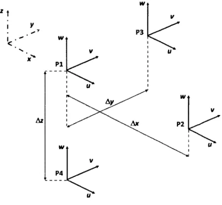
2004) 11 2.3 Schema of three-dimensional correlation of wind components u, v and w . . 12
2.4 Power spectral density (PSD) of u, v and w wind components of anemometer
2, bin CDS10, IREQ wind data 18 2.5 One-point u — w cross-coherence of: (a) bin CCSIO at z = 27 m; (b) bin
CCSIO at z = 20 m; (c) bin CCSIO at z = 10 m; (d) bin CDS10 at z = 27 m;
(e) bin CDS10 at z = 20 m; (f) bin CDS10 at z = 10 m 19 2.6 Two-point u-u coherence of: (a) bin CCS10 at Az = 7 m; (b) bin CCS10
for Az = 10 m; (c) bin CCS10 for Az = 17 m; (d) bin CDS10 for Az = 7ra;
(e) bin CDS10 for Az = 10 m; (f) bin CDS10 for Az = 17 m 21 2.7 Two-point w-w coherence of: (a) bin CCS10 at Az = 7 m; (b) bin CCS10
for Az = 10 m; (c) bin CCS10 for Az = 17 m; (d) bin CDS10 for Az = 7 m;
(e) bin CDS10 for Az = 10 m; (f) bin CDS10 for Az = 17 m 22 2.8 Two-point u-w coherence of: (a) bin CCS10 at Az = 7 m: (b) bin CCS10
for Az = 10 m; (c) bin CCS10 for Az = 17 m; (d) bin CDS10 for Az = 7 m;
(e) bin CDS10 for Az = 10 m; (f) bin CDS10 for Az = 17 m 23 2.9 PSD of u wind component of anemometer B, Cooper River wind data . . . 25
2.10 One-point and two-point u — w cross-coherence of anemometers B and B &
A, Cooper River wind data 25
3.1 FE model of parabolic structure for CPV solar tracker system 31
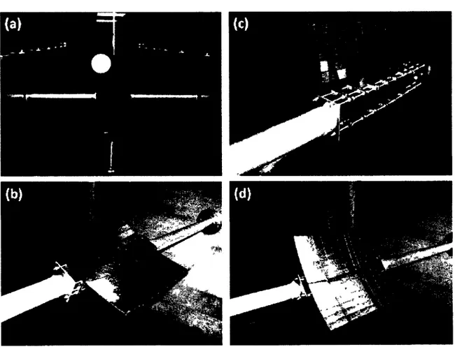
3.2 Sign convention for forces and moment 34 3.3 Sectional wind tunnel test of half of the parabolic structure: (a) overall
set-up; (b) additional stiffening for the back-up structure; (c) model with
the original plastic surface; (d) model with aluminum foil on its surface . . 35
3.4 Sign convention for the yaw and pitch angle 37
xviii LISTE D E S F I G U R E S
3.5 Wind pressure coefficient Cp for type Bl of Hosoya, N. et al. (2008) at wind
direction: (a) configuration 1,0 = 0°; (b) configuration 2, 0 = —30° . . . . 38
3.6 FE model with wind pressure for configuration 2 with 0 = - 3 0 ° 39
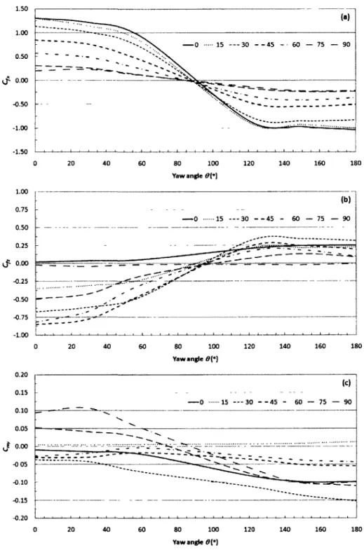
3.7 Steps required for fatigue analysis 41 3.8 Load coefficients of varied parabolic type structures 42
3.9 Load coefficients for varied yaw and pitch angles of the parabolic structure 44 3.10 Example of rainflow analysis result for 10-min sample of stress time history
from the rib member of the parabolic frame 47
4.1 Examples of guyed towers: (a) guyed Y tower; (b) guyed tower for
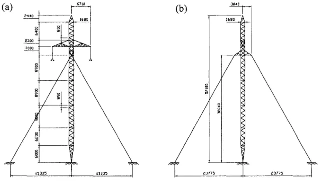
double-circuit TL; (c) guyed V tower; (d) cross-rope suspension tower 53 4.2 Geometry of the guyed lattice tower: (a) transverse view; (b) longitudinal
view. All dimensions in millimetres 55 4.3 Finite element (FE) model outline: (a) two-phase guyed tower: (b)
three-phase guyed tower 55 4.4 Structural response of two-phase guyed tower under wind loading U(10) =
35 m / s 56 4.5 Equivalent model verification: (a) truss model, first natural frequency of
the tower uiTi = 10.957 rad/s (1.744 Hz); (b) beam-column model, UT\ =
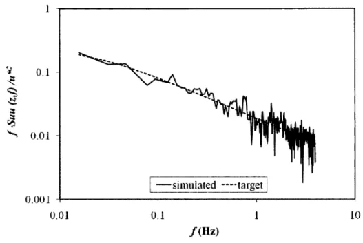
10.926 rad/s (1.739 Hz) ._ 58 4.6 Auto-spectrum of wind applied at mid-height of tower mast (U(10) = 35 m / s ) 63
4.7 Coherence function (normalized form of cross-spectral function) between
two points along the tower mast height (Az = 16.91 m, U(10) = 35 m/s) . 63 4.8 One 10 min sample of transverse bending moment of tower mast mid-height
z = 15.8 m of case 3P90w 67
4.9 One 10 min sample of transverse reaction of the tower mast of case 3P90w 68 4.10 Transverse bending moment: (a) Case 2P90w; (b) Case 3P90w; (c) Case
3P45w; (d) Case 2P90wi 72 4.11 Power spectral density (PSD) of bending moment of case 2P90w: (a) at guy
cable attachment point, z = 38.04 m; (b) at tower height, z = 20.24 m . . . 74 4.12 Wind factor for the tower for U{10) = 35 m / s for terrain type B: Gtotai is
the combined wind factor; Gmean is the factor due to the mean wind part;
Gturtmient is the factor due to turbulent wind part 77
4.13 Contribution from the TL components for the transverse bending moment:
(a) Case 2P90w; (b) Case 2P90wi; (c) Case 3P90w; (d) Case 3P45w . . . . 79
5.1 SDOF system used in this study 92 5.2 Nonlinear constitutive laws: (a) perfect elastoplastic; (b) bilinear with
strain hardening 92 5.3 Average of wind PSD for ten samples of the generated wind with Iu = 15 %
with confidence interval CI = 95 % 95 5.4 Hysteretic plot with generated wind for Iu = 15 %, wind sample 1, f\ = 0.5
Hz for elastic system (continuous gray line) and bilinear with a = 0.0,
LISTE D E S F I G U R E S x i x
5.5 Time history of generated wind with Iu = 15 %, sample 1, a = 0.0, f\ = 0.5
Hz and ft = 0.7 and fy = ft • 37.3 kN: (a) Total wind speed U{t); (b)
Displacement x and (c) Restoring force fs 97
5.6 Strength factor ft as a function of ductility /u, from ten samples of the gene-rated wind for Iu = 15 % with a = 0.0 for: (a) fx = 0.5 Hz; (b) fx = 1.0
Hz; and (c) / j = 2.0 Hz 98 5.7 Hysteretic plot - influence of damping for elastoplastic system where f\ =
0.5 Hz with ft = 0.7 with £ = 1 % (continuous grey line) and £ = 1.8 %
(continuous black line) 100 5.8 Comparison of specified ductility curves for a = 0.0 for generated wind with
Iu = 10 % and 20 % for: (a) n = 2 and (b) fi = 4 101
5.9 Specified ductility curves for a = 0.0 with varied frequency for generated
wind where: (a) Iu = 10 %; (b) Iu = 15 % and (c) /„ = 20 % 103
5.10 Hysteretic plot - influence of strain hardening with generated wind for /„ = 15 %, sample 1, where f\ = 0.5 Hz and ft = 0.7 for systems with a = 0
(continuous grey line) and a = 0.05 (continuous black line) 104 5.11 Comparison of specified ductility curves for generated wind with Iu = 15 %
for systems with a = 0.00 and a = 0.05 for: (a) \x = 2 and (b) ji = 4 . . . . 105 5.12 Elastoplastic system and its corresponding equivalent elastic system . . . . 109
5.13 Equivalent elastic system - frequency vs. ductility 110 5.14 Equivalent elastic system - damping vs. ductility 110 5.15 Total wind speed record V (continuous blue line) at height z = 10 m and
hourly wind direction (dotted grey lines) of studied winter storms: (a)
WS-dayl; (b) WS-day2 and (c) WS-day3 114 5.16 Component of wind speed perpendicular to surface Vx (where Vx = U)
and parallel to surface Vy of winter storm wind speed: (a) WS-dayl; (b)
WS-day2; (c) WS-day3 114 5.17 Wind PSD for WS-day2, 2nd hour, 17(10) = 15.12 m / s and z0 = 0.03 m for
the PSD models 115 5.18 Total wind speed record V (continuous blue line) at height z = 10 m and
hourly wind direction (dotted grey lines) of hurricanes: (a) Isabel-2003; (b) Ivan-2004; (c) Katrina-2005; (d) Rita-2005; and (e) Wilma-2005 (vertical
red lines represent hours used for this study) 117 5.19 Component of wind speed perpendicular to surface Vx (where Vx = U) and
parallel to surface Vy of hurricane wind speed: (a) Isabel-2003; (b)
Ivan-2004; (c) Katrina-2005; (d) Rita-2005; (e) Wilma-2005 118 5.20 Wind PSD for Isabel-2003, 14th hour, 17(10) = 28.6 m / s and z0 = 0.01 m
for the PSD models 119 5.21 Specified ductility - winter storm wind for: (a) // = 2 and (b) // = 4 . . . . 121
5.22 Specified ductility - hurricane wind for: (a) fi = 2 and (b) /i = 4 122 5.23 Ratio of /ie to / jn from varied / ] for: (a) nn = 2; (b) /in = 3 and (c) /un = 4 124
LISTE D E S F I G U R E S
B.l Mean and fluctuating wind components 145 B.2 Time history of wind speed: (a) Total wind speed U; (b) Turbulent wind
part u, v or w 146 B.3 Ensemble of time history records of wind speed 147
B.4 GUI of WindGen 165 B.5 Example to illustrate the wind field generated by WindGen 165
B.6 WindGen operating time for ID component 166
C.l FE model of multiple-span conductor 175 C.2 Types of insulators (Ducouret, X., 2005) 176 C.3 Types of towers (Hydro-Quebec. 2006) 178 C.4 Rigid link connectivity for equivalent beam-column guyed tower model (Kahla,
N.B., 1995) 179 C.5 Convergency of number of elements - in-plane symmetric modes 183
C.6 Convergency of number of elements - out-of-plane symmetric modes . . . . 183
C.7 Conductor self-damping ACSR conductor (Diana, G. et ai, 2000) 186
C.8 One panel section of a tower mast 192 C.9 Example of tension only stress-strain curve 193
C. 10 Stress-strain curves of an ACSR conductor (Asselin, J.M., 2006) 194
C.11 Stress-strain curve of steel (http://ocw.mit.edu/) 196 C.12 In-plane peak-to-peak displacement of mid-span with P = 100 • sin(u7£) . . 202
C.13 Out-of-plane peak-to-peak displacement of mid-span with P = 100 • sin(cZft) 202 C.14 In-plane peak-to-peak displacement of mid-span: P = PQ • sin(2.1078 • t) . . 203 C.15 Out-of-plane peak-to-peak displacement of mid-span: P = PQ • sin(0.8660 • t) 203
C.16 Comparison between 3 implicit methods in transient state 205 C.l7 Comparison between 3 implicit methods in steady state 205
D.l Two-phase guyed tower: first out-of-plane conductor mode shape. fCOnd{lop) =
0.12 Hz 209 D.2 Two-phase guyed tower : first in-plane conductor mode shape, fcond(lip) =
0.34 Hz 210 D.3 Two-phase guyed tower : second transverse tower mode shape, ftowC^r) =
2.81 Hz 210 D.4 Three-phase guyed tower : second transverse tower mode shape, ftowilr) —
1.72 Hz 211 D.5 Three-phase guyed tower : second transverse tower mode shape, ftowC^r) =
Liste des tableaux
2.1 Wind parameters of IREQ wind measurement for bins CCSIO and CDSIO . 17 2.2 Wind parameters of Cooper River wind measurement on January 27, 2003 24
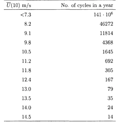
3.1 Maximum and minimum condition for the load coefficients 43 3.2 Summary of dynamic analyses results for the operational wind U(10) =
9.5 m / s 45 3.3 Equivalent wind speed for the fatigue load design 46
4.1 Cable properties 57 4.2 Loading cases .59 4.3 Applied wind points 60 4.4 Transverse moment (kNm) transient dynamic (TD) analyses of case 3P90w
(three-phase guyed tower under wind loading of U = 35 m/s) 66 4.5 Cable results for two-phase guyed tower (cases 2P90w and 2P90wi) . . . . 69
4.6 Cable results for three-phase guyed tower (cases 3P90w and 3P45w) . . . . 70
4.7 Tower mast reaction for the four loading cases 70 4.8 Natural frequencies and mode shapes of the TL structures under mean wind
for cases 2P90w and 3P90w and under dead load (values in parentheses) . 74
5.1 SDOF system variables for the parametric study 90
5.2 Variables for digitally generated wind 94
5.3 Winter storm wind variables 113 5.4 Hurricane wind variables 116
C.l Convergency of modes by number of elements 182 C.2 Comparison of un of the numerical result with the parabolic theory . . . . 184
C.3 Structural damping value at limit states (CECM-Comite technique 12 «Vent»,
1987) 185 C.4 Modelling damping in numerical model 189
C.5 Structural and material properties of typical conductors (Binette. L., 2006) 195
Chapitre 1
Introduction generate
Le but principal de la recherche est d'assembler les outils numeriques qui permettent l'etude dynamique des structures nonlineaires sous charges de vent. Ce projet est une reponse au besoin de l'industrie pour des outils numeriques qui prennent en consideration : (i) l'aspect dynamique non lineaire des structures et (ii) l'aspect aleatoire des charges de vent et d'autres caracteristiques notables de ce. chargement. L'importance de ces deux sujets a ete accentuee a la suite de grands evenements climatiques et de vents extremes ayant cause des dommages a plusieurs structures (Lelievre, C. et Chouinard,; L., 1998; Blake, E.S. et al., 2007).
Les objectifs principaux de cette etude sont :
- Mieux comprendre les effets de charges de vents extremes sur les structures en utilisant la dynamique transitoire;
- Proposer des methodes simplifiees qui permettent de bien representer le comportement dynamique nonlineaire sous charges de vent.
La contribution originale de cette etude est de rnontrer l'utilisation de la methode de calcul de vent en dynamique transitoire pour evaluer et analyser des structures complexes et pour repondre a des questions fondamentales sur la conception des structures sous charges de vent. La justification pour le choix de la methode dynamique transitoire ainsi que I'etat de l'art pour les analyses dynamiques des structures sous chargement climatique, specifiquc-ment pour des lignes aeriennes, sont detailles a l'annexe A. Cette revue bibliographique montre egalement les pratiques couramment utilisees par les autres etudes des structures
nonlineaires et complexes sous charges de vent.
Cette these est presentee comme une collection d'articles publies et soumis a des revues et des comptes rendus des conferences. La methodologie de cette etude comprend le de-veloppement des modeles numeriques de structures et de charges de vent en fonction du temps ainsi que l'utilisation de ces outils pour des etudes de structures complexes.
Les etapes de la methodologie sont les suivantes :
1. La preparation des donnees de vitesse de vent; pour modeliser les charges de vent, les etapes suivantes sont requises :
(a) Le developpement d'une base de donnees de mesures de vent reel, afin d'utiliser ces donnees pour des etudes connexes ou pour aider a etablir des modeles de vent de facon plus realiste pour la generation de vent numerique.
(b) La creation d'un logiciel pour la generation numerique de vent turbulent en fonction du temps. Le vent genere doit respecter la densite spectrale ciblee et prendre en consideration les correlations spatiales et temporelles du vent. L'uti-lisation de vent numerique permet une plus grande flexibilite dans l'etude des structures complexes et de grandes dimensions. Les details pour la methodologie de generation du vent numerique sont presentes a 1'annexe B.
2. Le developpement des modeles numeriques de structures non-lincaires et l'analyse dynamique transitoire : le modele de la structure doit prendre en consideration les non-linearites dus aux grands deplacements et les non-linearites de materiaux. Pour faciliter la creation de modeles de structures complexes, un processus efficace et systematique est mis en place.
Egalement, une methode d'analyse dynamique transitoire adaptee a l'analyse non-lineaire de la structure sous charge de vent a ete developpee, les etapes de cette methode sont donnees dans 1'annexe C.
Afin de mieux illustrer la methodologie d'etude de vent, la figure 1.1 montre un organi-gramme qui contient les etapes de calcul et d'analyse numerique. Dans cet organiorgani-gramme, les etapes sont donnees pour les charges de vent des structures nues (sans glace) et des structures couvertes de glace.
1. Introduction generate 3
- Le chapitre 2 presente I'etude de la correlation tridimensionnelle de vent basee sur des mesures in situ de vent.
- Le chapitre 3 decrit I'etude d'une structure parabolique a treillis, un systeme de concen-trateur solaire photovoltaique, afin de developper un concept structural robuste qui correspond a des criteres de conception stricts pour ce type de structure.
- Le chapitre 4 explique I'etude de pylones haubanes de lignes aeriennes .
- Le chapitre 5 decrit I'etude de systemes nonlineaires a un degre de liberte pour etablir le rapport entre la reduction de la resistance et la ductilite sous charges extremes de vent.
Verifications
•Auto correlation •Densitespectrale 'Correlation croisee 'Densite spectra le croisee
Z
Donnees V de charges /d e f l a t e /
Definir les coefficients de trainee pour la
structure nue
I
Calculer les forces de vent et • m o r t l « » m « n t
»«rodynamiqu«
Ajust«r lei coefficients de trainee pour des elements cou verts de glace et ajouter lepoidsdeflaee Analyses dynamiques transitoires
X
Resuhats—T"
Post^raitementI
Analyses Figure 1.1 -de ventChapitre 2
Correlation tri-dimensionnelle de
vent
2.1 Avant-propos
Auteurs et affiliation :
- F. Gani : etudiante au doctorat, Universite de Sherbrooke, Faculte de genie, Departement de genie civil.
- L-P. Parent : etudiant a la maitrise, Universite de Sherbrooke, Faculte de genie, Departement de genie civil.
- F. Legeron : professeur, Universite de Sherbrooke, Faculte de genie, Depar-tement de genie civil.
- S. Stoyanoff : expert en genie de vent, RWDI Consulting Engineers, Guelph, ON.
- P. Van Dyke : expert dans le domaine de lignes aeriennes, Institut de Re-cherche d'Hydro-Quebec (IREQ), Varennes, QC.
Titre anglais : Three dimensional wind correlation: Estimations from in situ measure-ments
6 2.1 A v a n t - p r o p o s
Titre francais : Correlation tri-dimensionnelle de vent : estimations a partir de mesures in situ
D a t e de publication : avril 2009
Etat de l'acceptation : une grande partie de ce chapitre a ete publiee et presentee lors de la conference; du materiel supplementaire a ete ajoute a la version originale de cet article afin de rnieux clarifier le sujet.
C o m p t e rendu : American Society of Civil Engineers (ASCE) Structures Congress '09, Austin, Texas, EU, 29 avril - 2 mai 2009.
R e s u m e :
II y a encore des lacunes dans les donnees de vent relatives aux correlations tridimensionnelles entre ses composants : dans le sens longitudinal, vertical et perpendiculaire du vent. Ces correlations sont importantes afin de mieux preciser les charges de vent sur des structures flexibles et longilignes, comme des ponts a longue-travee, des lignes aeriennes, etc. II est done souhaitable d'obtenir plus de renseignements relies a ces caracteristiques importantes de vent a partir de mesures de vent in situ. En utilisant des donnees de vent reel, les caracteristiques de correlation tridimensionnelle de vent sont evaluees et comparees aux modeles empiriques. Les modeles existants permettent de bien predire les caracteristiques du vent mesure in situ. Avec les resultats de cette etude, une amelioration du modele tridimensionnel de vent pourrait etre obtenue et utilisee pour la generation de donnees numeriques de vent.
Mots-cles : coherence, -croise, densite spectrale, anemometre, sens longitudinal,
vertical, perpendiculaire au vent.
Abstract:
For wind load design, there is still a certain lack of full scale data in the cross-properties among along-, vertical- and across-wind directions. These cor-relations are important for precise prediction of wind loads on flexible, line-like
2. Correlation tri-dimensionnelle de vent 7
structure such as long-span bridges, transmission lines, etc. It is then desi-rable to obtain more information related to these important wind parameters based on in situ wind measurements. Using these real wind data, the three-dimensional correlational properties of the wind components were evaluated and compared to the available empirical models. A relatively good fit were found between the calculated results and empirical models. The results from this study could be used to improve the current three-dimensional wind corre-lational models for the purpose of digitally generating wind data.
Key words: cross-, coherence, anemometer, along-, vertical-, across-wind.
2.2 List of variables
Variable Definition
9 — 2
C o h ^ , Cohee coherence function, estimate of coherence for wind components e = u, v or w
Cy, Cz exponential decay coefficients
/ frequency (Hz)
Ic intensity of turbulence (Ie = at/U(z)) of wind component e = u, v or w (%)
Lu, Lw length scales of turbulence in x-direction relating to u and w components (m)
n coefficient for confidence interval calculation N number of samples
s standard deviation from the available samples
Sec, Set spectral density function, estimate of spectral density for components e ( m2/ s )
tn-,a/2 Student's t distribution value for n — N - 1
u, v, w fluctuating or gust components of wind speed along x, y and z axes ( m / s ) U(z) mean wind speed at height z ( m / s )
x, y , z system of rectangular cartesian coordinates with z-axis
defined in the direction of mean wind and z-axis vertical (m)
x, nx mean value from the available samples; real mean value
z effective height above ground obstructions (m) ZQ surface roughness parameter or roughness length (m) a coefficient to define the confidence interval
8 2.3 I n t r o d u c t i o n
2.3 Introduction
The correlation properties of the wind (expressed as wind coherence in frequency domain representation) are important for precise prediction of response to wind for flexible, line-like structures such as long-span bridges, telecommunication towers, wind turbine towers and transmission lines. Although extensive research including field measurements has been carried out in the past, there is still a lack of data that defines complete correlation between the components of wind turbulence. Whereas correlations in the along-wind mean direction are more or less clearly understood and well defined, there is a certain shortage of full scale data in the cross-properties among along-, vertical- and across-wind directions. It is therefore desirable to obtain more information related to these important wind parameters based on field measurements.
The objective of this paper is to provide more information on this subject based on two in situ wind measurements. One set of data was obtained during the measurements under-taken for the New Cooper River Bridge, Charleston, South Carolina. The second set was the wind measured on the experimental line of Hydro-Quebec Research Institute (IREQ). The first site is characterized by open water for wind directions normal to the bridge crossing, close to south and north wind. The second site is an open terrain.
For both wind measurements, three-dimensional (3D) ultrasonic anemometers were used. Based on the available wind data, the correlations between along-wind (u), across-wind
(v) and vertical (w) turbulence components were evaluated at the same measurement
point, and as well, at separated measurement points. Since the vertical and across-wind structural responses depend on the turbulence fluctuations in the respective directions, knowledge of their cross correlations would help improve the response estimations.
In addition, the effect of separation distance on correlation was also analyzed. The esti-mation of spatial effects on correlation can be used to refine the site specific wind loading over the structural span of power lines or bridges, or height for towers. The results for wind spectra and the coherence for 3D wind will be presented, as well as comparison with the available empirical wind models.
2. Correlation tri-dimensionnelle de vent 9
f
®
Figure 2.1: Set-up of five ultrasonic anemometers for wind measurements on the experi-mental line of IREQ
2.4 W i n d measurement sites
2.4.1 E x p e r i m e n t a l line of I R E Q
This data set was provided by Hydro-Quebec Research Institute (IREQ). The set comprises a one month continuous wind measurement (March 20 to April 19, 2008) obtained from the expeiimental line facility of IREQ in Varennes, Quebec, Canada. The site is essentially a flat, covered with snow terrain (roughness length z$ « 0.01 to 0.03 m). During the measurement period, the prevailing wind direction was almost normal to the experimental line.
The wind measurement set-up consists of an array of five ultrasonic anemometers, mounted on three pylons, which are arranged parallel to the longitudinal direction of the experimen-tal line. The distance between each pylon is 75 m. The setting of this wind measurement is shown in figure 2.1. The five anemometers were mounted as follows anemometers 1, 3
10 2.4 W i n d m e a s u r e m e n t sites
and 5 were elevated at z = 20 m; anemometer 2 was at z = 27 m; and anemometer 4 was at z = 10 m height.
The data were recorded in ten-minute segments. The wind measurement was recorded continuously during the measurement campaign, 24 hours per day, for 30 days. Each ten-minute segment (one sample) contains approximately 18000 data points, recorded at a sampling frequency of 30 Hz.
The available samples were grouped into bins, according to the mean wind speed recorded at the height z = 10 m, c/(10) and the mean wind direction 9. For the mean wind speed, the bin interval was set to be 5 m/s. For the mean wind direction, the interval was 30°. Following the accepted notation, a bin named CCS10 would contain samples with mean wind speed within 10 < (7(10) < 15 m / s and mean wind direction in the range of 270° < 9 < 300°, i.e., almost normal to the experimental line alignment. Table 2.1 in section 2.6.1 provides the bins used in this study as well as their wind parameters.
2.4.2 Cooper River site
This data set was available for this study by the courtesy of the bridge designers Parsons Brinckerhoff, and the bridge owner South Carolina DOT, USA. The wind measurement was done in order to confirm the turbulence properties on the Cooper River site, corres-ponding to a mix of a suburban and open water type of terrain (estimated combined roughness length z0 = 0.02 m). Data from December 2002 to April 2003 were available for
analysis and were detailed in Kelly, D.R. (2004). The wind measurement was relatively uninterrupted.
In this wind measurement, three ultrasonic anemometers were installed on the old truss bridges, namely Silas Pearman and Grace Memorial, as shown in figure 2.2. The elevations of these anemometers were: 67.7 m and 69.7 m for anemometers A & B (Grace Memo-rial) respectively; and 67.5 m for anemometer C (Silas Pearman). Each anemometer was installed on a 3 m long guyed mast. The distance between anemometer A and B is
Ay = 53.3 m. The distance between anemometer B and C is Ax = 94 m.
Data from the three anemometers were collected in cycling fashion by ten-minute segments. The first (e.g. 9:00 to 9:10) and fourth (e.g 9:30 to 9:40) segment readings of every hour from all three anemometers were recorded at sampling frequency of 2.5 Hz. During the
2. Correlation tri-dimensionnelle de vent 11
Figure 2 2 Set-up of three ultrasonic anemometers for wind measurements on the Cooper River Bridge site - these old bridges were later demolished (Kelly, D R , 2004)
1 2 2 . 5 One-point and two-point cross-coherence of t h e w i n d c o m p o n e n t s u, v, w
second (9:10 to 9:20) and fifth segments (9:40 to 9:50), measurement from anemometers A and B were recorded, at sampling frequency of 4 Hz. While for third (9:20 to 9:30) and sixth (9:50 to 10:00) segments, only anemometer B was recorded, at sampling frequency of 8 Hz.
2.5 One-point and two-point cross-coherence of t h e
wind components u, v, w
A complete 3D correlation model will be helpful in realizing a more realistic numerical wind loading generation. Nonetheless, there is an important shortcoming in the com-pleteness of the empirical formulae available, to represent the cross-correlation between longitudinal and vertical/lateral turbulence components. The general consensus for the cross-properties among the other components is that being weaker, they are less impor-tant for response estimations. The knowledge in this subject is imporimpor-tant considering the
Az
2. C o r r e l a t i o n t r i - d i m e n s i o n n e l l e d e v e n t 13
coupled interaction of wind-sensitive structures.
For horizontal structural elements, such as bridge deck or power lines, u—w cross-properties are controlling the magnitude of the across-flow loads, whereas for vertical structural el-ements, such as towers, u — v cross-properties would be the important ones. Without a reliable cross-coherence model, the wind-structure interaction response would not reflect the actual structural behaviour. Studies that included the along-wind and vertical com-ponents mostly neglected the one-point and two-point cross-coherence as a simplification and/or due to unavailability of reliable models. A schema that illustrates the three di-mensional correlations and spatial separations of wind measurement points is shown in figure 2.3.
From the preliminary studies, and supported by previous studies for the three-dimensional wind correlation (e.g. Saranyasoontron, K. et al. (2004); ESDU-86010 (1986)), it was found that the estimated same point cross-coherence between the along-wind and across-wind
u — v SLS well as the across-wind and the vertical component v — w are far less significant
than the along-wind and vertical wind u — w. Therefore, the present study focused on the one-point and two-point cross coherence of u—w for vertical Az and lateral Ay separations.
The available coherence empirical models are used to compare with the estimated cohe-rence from the wind records. For the calculation of the cross-cohecohe-rence u — w, the cohecohe-rence model from the same components u — u and w — w are also required. Several available cohe-rence functions are evaluated in this study. The one-point u — w cohecohe-rence by Solari, G. et Piccardo, G. (2001) and the two-point u — w cross-coherence of Minh, N.N. et al. (1999) were retained for this study. For the u — u coherence, the Davenport model (Davenport, A.G., 1968) was used. For the vertical components coherence, equation by Bowen, A.J.
et al. (1983) was adopted. The coherence functions used in this study are provided in
section 2.5.3.
2.5.1 Coherence from t h e wind records
From the available wind sample records, the coherence estimate can be calculated for the wind components of interest (u,v and w). The coherence function is a function of frequency with values between 0 and 1 that indicates how well two stationary random processes correspond to each other at each value of frequency.
142.5 One-point and two-point cross-coherence of t h e w i n d c o m p o n e n t s u, v, w
— — 2
The estimate of the squared coherence function Coh (/) of two stationary random pro-cesses can be expressed as (Bendat, J.S. et Piersol. A.G., 2000):
Coh2(/) = ^hf (2.5.1)
where Slalb is the estimate of the cross-spectrum density of ea and e^; the subscript a and
b are for the two components analysed; e is the wind component of interest, those are u,v
or w; Sta and Sib are the estimates of the auto spectra densities.
2.5.2 Confidence intervals
The results provided for the parameters of interest (e.g. wind PSD or coherence) from the mean of the available samples are estimates of the 'real' parameters of interest. A more meaningful procedure for estimating parameters of random variables involves the estimation of an interval (Bendat, J.S. et Piersol, A.G., 2000).
For the case of the mean value estimate, a confidence interval can be established for the mean value fxx based on the mean value from the available samples x as follows (Bendat,
J.S. et Piersol, A.G., 2000):
_ s tn\a/2 , _ , s tn;a/2
x ^ _ < n < x H ~ - (2.5.2)
where s is the standard deviation from the available samples; tn;ft/2 is the Student's t
distribution value for n = N — 1; N is the number of samples.
In the present study, a = 0.05, therefore the confidence coefficient of 100 (1 — a) %— 95 % is used for calculating the interval band of the results.
2.5.3 Available empirical models
The available empirical models from previous studies were used to compare the estimated coherence functions from the wind records.
2. Correlation tri-dimensionnelle de vent 15
The square root of the coherence function for two-point of the same wind component, as proposed by Davenport, A.G. (1968) is defined by:
c„
h(/). exp (_mc,*
fr
+ {c.*vrr\
(2.
5,
3)where Cz and Cy are the exponential decay coefficients; Az and Ay are the distances
between point a and b; U is the mean wind speed. In the present study, the exponential decay coefficients for the u — u component for the vertical and lateral separations are:
Cz = 10 and Cy = 16 (Simiu, E. et Scanlan, R., 1996).
For the present study, it was found that the above equation did not provide good represen-tation for the two-point w — w coherence. Therefore, another empirical model by Bowen, A.J. et al. (1983) was used instead. The equations related to this model are:
Coh2WaWb(f,Az) = c-exp-a'™ (2.5.4)
where:
Az
c = 1 - 0 . 5 — (2.5.5)
Az
-a'zn = 4 + 10— (2.5.6)
One-point u — w cross-coherence from Solari, G. et Piccardo, G. (2001) is:
Coh^
o(/) = - - J -
1_ = = (2.5.7)
*u
au,
0^i+QA[fL
v/U(z)]
2 where: ««.«««(*) = Auawa \/ftu{z)ftw(z) (2.5.8) AUaWa = l.U[Lw/LX21 (2.5.9) ftu = 6- 1.1 t a n - ^ l n ^ o ) + 1.75] (2.5.10)16
2.6 Results and discussions
in which L
w/L
u= 0.08 and cr
w/a
u= 0.55 for Kaimal spectra;
and the integral scale length L
uis defined by:
L
u= 5.67 z (2.5.12)
Two-point u — w cross-coherence proposed in Minh, N.N. et al. (1999) is expressed as:
Cohl
aWb(f) =
2S*\fi
{£
{f)[Coh
UaUb(f) + Coh
WaWb(f)} (2.5.13)
in which the first term of the equation is the one-point u — w cross-coherence.
2.6 Results and discussions
2.6.1 Results from I R E Q wind m e a s u r e m e n t
For the IREQ wind data, the one-point and two-point u — w cross-coherence were derived
from pylon with anemometer 2, 3 and 4. In the present study, the cross-coherence for
varied vertical separations between anemometer 2, 3 and 4 were examined in details in
order to study the two-point u — w cross-coherence. Anemometer 2 is at height z = 27 m,
anemometer 3 is at height z = 20 m and anemometer 4 is at height z = 10 m. Hence, the
vertical separations studied here are Az =• 7, 10 and 17 m.
Comparisons were made for the bins with largest values of U(10) and wind direction almost
normal to the experimental line: CCS10 and CDS10. The parameters related to these two
bins are given in table 2.1. For wind loading design purposes, wind speed of interest would
be (7(10) > 20 m/s. During the measurement period, the highest mean wind were in
the range of 15 to 20 m/s in bin CDS10, where only six samples are available. More
samples, with relatively high mean wind speed (range of 10 to 15 m/s), are available in
bin CCS10. Nonetheless, as summarized in ESDU-86010 (1986), the use of wind samples
with (7(10) ~ 10 m/s are accepted to develop theoretical basis of wind models, as this is
the case for the large part of the available studies for wind models.
2. Correlation tri-dimensionnelle de vent 17
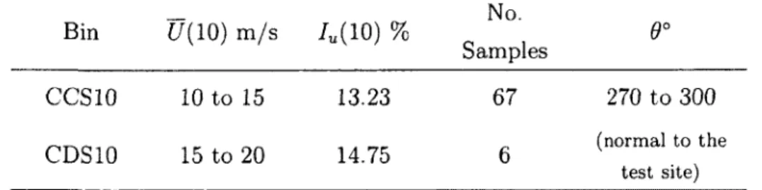
Table 2.1: Wind parameters of IREQ wind measurement for bins CCSIO and CDSIO
Bin
CCSIO
CDSIO
U{10) m/s
10 to 15
15 to 20
/
u(10) %
13.23
14.75
No.
Samples
67
6
9°
270 to 300
(normal to the test site) Note: (7(10) is the mean wind speed; /u(10) is the turbulenceintensity; 0 is the mean wind direction
For all the results given in this section, the term 'estimate' refers to the calculated mean of the available samples per bin. The confidence interval band for CI = 95 % is also presented in the results. The estimates are calculated from the ten-minute samples. Each sample is divided into six subsegments with 50 % overlapping, following recommendations in Bendat, J.S. ctPiersol, A.G. (2000).
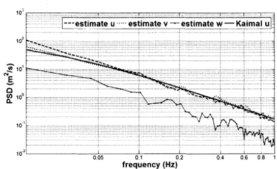
Before proceeding with the coherence calculations, the wind power spectral densities (PSD) of the measured data were calculated for the bins of interest. From the complete results of the PSD evaluation, it was concluded that the measured data agreed quite well with the Kaimal spectra. An example of the wind PSD plot is shown in figure 2.4 for anemometer 2 at z = 27 m for u, v and w components, as well as the theoretical PSD of u component from Kaimal (Kaimal, J.C. et al, 1972). In this figure, the average of u component of bin CDS10 for / < 0.1 is higher than the theoretical prediction, for / > 0.1, the agreement is good. It can also be observed that the PSD of v has comparable magnitude as u component, while the w component has lower magnitude.
2.6.1.1 One-point u-w coherence
The one-point u — w cross-coherence for the two bins studied here is shown in figure 2.5(a) to (c) for bin CCS10 for height z = 27, 20 and 10 m respectively; and (d) to (f) for bin CDS10 with the same heights as bin CCS10. In this figure, the dotted blue lines are the confidence interval band CI = 95 %, the continuous blue line is the mean from the samples. The theoretical one-point u — w cross-coherence (dot-point green line) is calculated using equation 2.5.7 (Solari, G. et Piccardo, G., 2001). The agreement between
18 2.6 Results and discussions
—estimate u estimate v — estimate w — Kaimal u :
1 0-'i 1 J 1 1 1 1 — i
0.05 0.1 0.2 0.4 0.6 0.8 1 frequency (Hz)
Figure 2.4: Power spectral density (PSD) of u, v and w wind components of anemometer 2, bin CDS10, IREQ wind data
measured and the theoretical curves was found to be satisfactory for bins CCS10 (67 samples) and CDS10 (6 samples). It can be concluded that the one-point u — w cross coherence proposed by Solari, G. et Piccardo, G. (2001) predicts well the real wind u — w components correlation.
2.6.1.2 Two-point u — u and w — w coherence
In order to obtain the theoretical two-point u — w cross-coherence, it was also necessary to adopt reasonable models for the two-point coherence of the u—u and w—w components. To verify the appropriateness of the coherence functions, they are compared to the coherences estimated from the wind records.
The u — u two-point coherence are presented in figure 2.6(a) to (c) for bin CCS10 with
Az — 7, 10 and 17 m respectively; and (d) to (f) for bin CDS10 with the same vertical
separations as bin CCS10. For these vertical separations, the u — u coherence, which is the square of equation 2.5.3 (Davenport, A.G., 1968). showed a very good agreement with the theoretical values for Az = 7 and 10 m. For Az = 17, for bin CCS10 the theoretical curve over predicts the coherence; while for bin CDS10, the theoretical coherence does not
2. Correlation tri-dimensionnelle de vent 19
CCS10 (0(10) = 10 to 15 m/s) CDS10 (0(10) = 15 to 20 m/s)
0.1 0.2 0.3 0.4 0.5 5!i M 0.3 0.4 o'5 Frequency (Hz) Frequency (Hz)
Figure 2.5: One-point u — w cross-coherence of: (a) bin CCSIO at z = 27 m; (b) bin
CCSIO at z = 20 m; (c) bin CCS10 at z = 10 m; (d) bin CDSIO at z = 27 m; (e) bin
CDSIO at z = 20 m; (f) bin CDSIO at z = 10 m
20 2.6 Results and discussions
follow the estimation mean very well, but it is still within the confidence interval.
The w — w two-point coherence are shown in figure 2.7 for bins CCSIO and CDSIO with the same vertical separations as the previous figure. For the w — w component, the estimated coherence was compared to equation 2.5.4 (Bowen, A.J. et al., 1983). For bin CCSIO, the theoretical prediction is always higher than the coherence from the real wind. A better agreement was observed for bin CDSIO, even though there were relatively fewer (6) samples available. This result highlighted the fact that stronger correlation between u and w components exists for samples with higher wind speed. In addition, it seems that a better vertical two-point coherence model is required for better prediction of the real wind.
2.6.1.3 Two-point u — w coherence
The theoretical two-point u — w coherence can be obtained after calculating the theoretical one-point u — w cross-coherence, and the u — u and w — w coherences by using equa-tion 2.5.13 (Minh, N.N. et al, 1999). The results of the two-point u — w cross-coherence are shown in figure 2.8(a) to (c) for bin CCSIO with Az = 7, 10 and 17 m respectively; and (d) to (f) for bin CDSIO with the same vertical separations as bin CCSIO. From this figure, it can be observed that for Az = 7 m ((a) and (d)) at the lower frequency range of less than 0.2 Hz, the measured two-point u — w cross-coherence fit the theoretical curve relatively well, but for the higher frequency range, the measured values are higher than the theoretical prediction.
For bin CCSIO in (b) and (c) of the figure, it can be seen that the theoretical coherence only predicts well at very low frequency range (less than 0.05 Hz), elsewhere, the estimated coherence are higher. The estimated coherence value of « 0.1 for / > 0.1 Hz is obtained from all vertical separation distances for bin CCS10 and CDS10. For bin CDS10, despite the reasonable fit, there are larger deviations between measured and theoretical values. From figure 2.5 and 2.8, it can be observed (as expected) that the one-point u — w cross-coherence is larger than the two-point u — w cross-cross-coherence, due to a drop in correlation of the wind gusts in the two separated measurement stations.
The two-point u — w cross-coherence is the magnitude of 0.1 to 0.2 for very low frequency ( / < 0.1). For small vertical separation and stronger wind speed, stronger correlation
2. Correlation tri-dimensionnelle de vent 21 CCS10 (0(10) = 10 to 15 m/s) CDS10 (0(10) = 15 to 20 m/s) 01 02 03 0 4 0 5 Frequency (Hz) 01 02 03 04 05 Frequency (Hz)
Figure 2 6 Two-pomt u — u coherence of (a) bin CCSIO at Az — 7 m, (b) bin CCSIO for
Az = 10 m, (c) bm CCSIO for Az = 17 m, (d) bin CDS10 for Az = 7 m, (e) bm CDSIO
22
2.6 Results and discussions
0 8 • 0 6 • 02 0 1 0 8 Eos • > < 0 2 CCS10(0(10) »*fc^ « _ _ _ _ _ •"" - * = 10 to 15 m/s) ' MttimM 86% a - Bovwn «t 0 (1983) *"*.. " ^ > — y ^ \ , ^^^v-Iw
• • CDS10 (0(10) = 15 to 20 m/s) 01 02 03 04 OS 02 03 04 05 (c) ^ . • 1 ^ -=?»• • '• % ^ a i 01 Frequency (Hz) 02 03 04 05 0 8 02 03 04 OS (•) 01 02 03 04 05 Frequency (Hz)Figure 2 7 Two-point w — w coherence of (a) bm CCSIO at Az = 7 m, (b) bin CCSIO for
Az = 10 m, (c) bin CCSIO for Az = 17 m, (d) bin CDSIO for Az = 7 m, (e) bin CDSIO
2. Correlation tri-dimensionnelle de vent 23 CCS10 (0(10) = 10 to 15 m/s) CDSIO (0(10) = 15 to 20 m/s) 01 0.2 03 04 0.5 Frequency (Hz) 01 02 03 04 05 Frequency (Hz)
Figure 2.8: Two-point u-w coherence of: (a) bin CCSIO at Az = 7 m; (b) bin CCSIO for Az = 10 m; (c) bin CCSIO for Az = 17 m; (d) bin CDSIO for Az = 7 m; (e) bin CDSIO for Az = 10 m; (f) bin CDSIO for Az = 17 m
24 2.6 Results and discussions
Table 2.2: Wind parameters of Cooper River wind measurement on January 27, 2003 Anemo-meter A B C z (m) 67.70 69.70 67.50 U(z) m / s 10.19 10.23 8.69 In (%) 9.90 10.16 19.12
h (%)
9.56 10.26 11.47 Iw (%) 7.37 7.13 9.42 No. Samples 24 16 8will likely to exist. Hence, for better evaluation of this coherence, more samples of strong wind are needed.
2.6.2 Results from C o o p e r River site m e a s u r e m e n t s
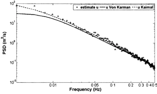
From the available data sets, the wind normal to Grace Memorial Bridge was retained for analysis. In the present study, lateral separation between anemometers A & B, Ay = 53.3 m, was investigated. The key parameters of this data set were derived by Kelly, D.R. (2004), as summarized in table 2.2. As figure 2.9 shows, the PSD of anemometer B (wind storm of January 27, 2003) is in a better agreement to the theoretical formula of Kaimal (Kaimal, J.C. et al., 1972) than to the von Karman (von Karman, T., 1948) spectrum.
For the one-point and two-point u — w cross-coherence, the calculation results are shown in figure 2.10. In this figure, it can be seen that the overall maximum magnitude between the measured and the theoretical coherence are similar. For the one point u — w cross-cohe-rence, the measured data showed lower values at the lower frequency range but overall, the theoretical curve seems to envelop well this data set. While for the two-point u — w cross-coherence, almost for the whole frequency range, the measured values are higher than the theoretical value. The weak coherence level implies that due to the relatively low wind speeds, the ambient noise in the turbulence (uncorrelatcd gusts) was likely dominating.
2. Correlation tri-dimensionnelle de vent
25
10' 10' •52£ io°
Q Q . 10" 10"'l" * - „ * 4 estimate u — u Von Karman
^ ^ < % A A^CSS&A I : . . I I I — ii Kaimal -' 1 1 0 01 0 05 0 1 0 2 0 3 0 40 5 Frequency (Hz)
Figure 2.9: PSD of u wind component of anemometer B, Cooper River wind data
0 35 0 30 0 25 j 0 2 0 JC