HAL Id: hal-02286129
https://hal.archives-ouvertes.fr/hal-02286129
Submitted on 13 Sep 2019
HAL is a multi-disciplinary open access
archive for the deposit and dissemination of
sci-entific research documents, whether they are
pub-lished or not. The documents may come from
teaching and research institutions in France or
abroad, or from public or private research centers.
L’archive ouverte pluridisciplinaire HAL, est
destinée au dépôt et à la diffusion de documents
scientifiques de niveau recherche, publiés ou non,
émanant des établissements d’enseignement et de
recherche français ou étrangers, des laboratoires
publics ou privés.
Estimation of static and dynamic urban populations
with mobile network metadata
Ghazaleh Khodabandelou, Vincent Gauthier, Marco Fiore, Mounim El
Yacoubi
To cite this version:
Ghazaleh Khodabandelou, Vincent Gauthier, Marco Fiore, Mounim El Yacoubi.
Estimation of
static and dynamic urban populations with mobile network metadata.
IEEE Transactions on
Mobile Computing, Institute of Electrical and Electronics Engineers, 2019, 18 (9), pp.2034-2047.
�10.1109/TMC.2018.2871156�. �hal-02286129�
Estimation of Static and Dynamic Urban
Populations with Mobile Network Metadata
Ghazaleh Khodabandelou, Vincent Gauthier, Marco Fiore, Senior Member, IEEE, Mounim El-Yacoubi
Abstract—Communication-enabled devices routinely carried by individuals have become pervasive, opening unprecedentedopportunities for collecting digital metadata about the mobility of large populations. In this paper, we propose a novel methodology for the estimation of people density at metropolitan scales, using subscriber presence metadata collected by a mobile operator. Our approach suits the estimation of static population densities, i.e., of the distribution of dwelling units per urban area contained in traditional censuses. More importantly, it enables the estimation of dynamic population densities, i.e., the time-varying distributions of people in a conurbation. By leveraging substantial real-world mobile network metadata and ground-truth information, we demonstrate that the accuracy of our solution is superior to that granted by state-of-the-art methods in practical heterogeneous urban scenarios.
Index Terms—Population estimation; static population density; dynamic population density; mobile network metadata.
F
1
I
NTRODUCTIONMobile network operators collect a profusion of metadata from the digital communication activity of their subscribers. They are in a position to extract significant new knowledge on human behaviors at heterogeneous scales, ranging from single individuals to large populations. Examples abound, and are comprehensively reviewed in [1]: they include original insights on mobility laws [2], patterns of daily commuters [3], dynamics of infective disease epidemics [4], or people reaction to disaster situations [5]. Mobile network operators can then leverage such information to develop metadata-driven value-added services, for, e.g., transport analytics [6] or location-based marketing [7].
Our work focuses on the use of mobile network meta-data for the estimation of population density in urban regions, which is a paramount information for informed planning in metropolitan areas by local authorities. Tradi-tional censuses are carried out at regular time intervals in all developed countries, and allow determining static popula-tion densities, i.e., the spatial distribupopula-tions of citizens’ places of habitation or dwelling units. However, these censuses are complex to organize and expensive to run, which limits their periodicity to a few years in best cases [8]. Instead, metadata collected by mobile network operators is fairly inexpensive to obtain, and covers large portions of the population [1]. A reliable estimation of the static population density based on such metadata would eliminate the limitations of conven-tional survey-based approaches [9], [10].
In addition, mobile network metadata can be retrieved and analyzed with minimum latency. This paves the road to the characterization of dynamic population densities, i.e., of the instantaneous distributions of individuals that evolve as people move over time in the region of interest. The automated, near-real-time estimation of population density dynamics has inestimable value in supporting innovative
G. Khodabandelou, V. Gauthier and M. El-Yacoubi are with SAMOVAR,
Telecom SudParis, CNRS, Universit´e Paris Saclay, 91000 ´Evry, France.
E-mail: name.surname@telecom-sudparis.eu.
M. Fiore is with CNR, 10129 Torino, Italy. E-mail: marco.fiore@ieiit.cnr.it.
services for instance to transport planning, large event orga-nization, public safety, or law enforcement.
The utility of a reliable estimation of population distri-butions based on mobile network metadata has generated a flurry of recent studies on the subject [11], [12], [13], [14], [15], which we review in Section 8. Our work has the following advantages over such previous proposals.
(i) Our design is based on a number of original metadata filters that significantly improve the accuracy of the popula-tion density estimate. The filters operate on subscriber pres-ence, which we show to be a better proxy of the population density than other classes of mobile network metadata.
(ii) We exploit a novel multivariate relationship of pop-ulation density, subscriber presence and subscriber activity level for the estimation of dynamic population densities.
(iii) When confronted with ground-truth data in multiple urban scenarios, our solution achieves good accuracy in estimating static and dynamic population densities. Specif-ically, it consistently outperforms current state-of-the-art approaches in both cases, and generates reasonable dynamic representations of the population distribution that allow, e.g., appraising attendance at sports and social events.
(iv) Estimates of the dynamic population distribution ob-tained with our proposed model are openly accessible [16]. The datasets describe one month of population density fluctuations in the cities of Milan, Rome and Turin.
The paper is organized as follows. Section 2 describes our reference datasets. Section 3 presents the model for static population estimation, which is assessed in Section 4. Model refinements for the dynamic case are explained in Section 5 and evaluated in Section 6. Comparisons with the state-of-the-art are in Section 7, and related works are reviewed in Section 8. Section 9 concludes the document.
2
D
ATASETSWe leverage several datasets made available by Telecom Italia Mobile (TIM) within their 2015 Big Data Chal-lenge [17]. We focus on three major conurbations in Italy, i.e., Milan, Turin and Rome. For each city, we retrieve metadata about the mobile traffic activity (presented in Section 2.1),
04:00 04:15 04:30 04:45 05:00
call (in/out) sms (in/out) data (send/received)
A B C ACTUALLOCATION ACTIVITY ESTIMATEDLOCATION D A C D
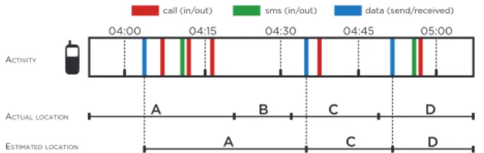
Fig. 1: Example of subscriber location estimation. Network events of a mobile phone (top) allow approximating the cell where the user is located (bottom). This entails an error with respect to the actual position of the user in time (middle). as well as ground-truth census data on the local population distribution (Section 2.2). We then infer information on land use from the mobile network metadata itself (Section 2.3).
2.1 Mobile network metadata
The mobile network metadata provided by TIM covers the months of March and April 2015, and describes the volume of traffic divided by type (incoming and outgoing voice calls, incoming and outgoing text messages, and Internet sessions), as well as the approximate presence of sub-scribers. These features are commonly available to mobile network operators from Call Detail Records compiled for billing purposes, hence they represent a sensible choice for developing an estimator of population density that is reusable. All metrics are aggregated in time and space. In time, the metadata is totaled over 15-minute time intervals. In space, metrics are computed over an irregular grid tes-sellation, whose geographical cells do not overlap and have sizes ranging from 255ˆ325 m2to 2ˆ2.5 km2. The number
of cells is 1419 for Milan, 571 for Turin and 927 for Rome. While voice, text, and Internet traffic volumes are di-rectly computed from the recorded demand, the presence in-formation is the result of a simple preprocessing performed by the mobile network operator. Basically, each subscriber is associated to the geographical cell where he last inter-acted with the network for any purpose, which includes issuing or receiving a voice call, sending or receiving a text message, or establishing a new Internet data session. As each type of activity provides additional localization information, including them all in the calculation makes the presence information more accurate. If a user is first detected within cell A, then he performs some activity in cell B at time t1, and his latest action is recorded in cell C
at time t2, his location will be as follows: for t ď t1, the user
is positioned in A; for t1 ă t ď t2, he is in B; for t ą t2,
and until he performs an action in a different cell, he is in C. Figure 1 shows an example of this user location estimation process. The presence metadata is then inferred by counting subscribers in each cell, at every 15 minutes.
2.2 Population distribution
Our ground-truth data for the static population distribution comes from the 2011 housing census run by ISTAT, the national organization for statistics in Italy. It includes pop-ulation counts, measured in terms of families, cohabitants, persons temporarily present, domiciles, and other types of lodging and buildings, for each administrative area.
To ensure spatial consistency between the mobile net-work metadata and the census data, we proceed as follows.
Let us denote as Uj the total number of inhabitants in the
administrative area j, and as Aj its surface. The population
density ρiin a geographical cell i, defined in Section 2.1, is
then computed by assuming a uniform spatial distribution of inhabitants in each administrative area, as
ρi“ 1 Si K ÿ j“1 Uj SiX Aj Aj (1) where Siis the surface of cell i, K denotes the total number
of administrative areas, and SiX Ajstands for the
intersec-tion surface of cell i and administrative area j.
2.3 Land use
Land use information is critical to the accurate estimation of population densities, and is regularly employed in the re-cent literature [14], [15]. We leverage the operator-collected data itself to classify the geographical cells based on their primary land use. To that end, we employ MWS, which is the current state-of-the-art technique for land use detection from mobile network metadata [18].
MWS computes, for each spatial cell of the target region, a mobile traffic signature, i.e., a compact representation of the typical dynamics of mobile communications in the considered cell. Specifically, MWS signatures are computed as the median voice call and text activity in a cell recorded at every hour of the week. Signatures are clustered based on their shape, using a classical hierarchical algorithm on top of a correlation-based signature similarity measure. The output clusters group cells with similar types of human activities, i.e., belonging to a same land use. Averaging the signatures of all cells in a specific cluster allows defining characteristic signatures associated to each land use, which are shown to be city-invariant: hence, once the characteristic signatures are identified, MWS can detect land use regions by solely using mobile network metadata. When applied to our reference datasets, MWS classifies urban areas into five land uses: residential, office, touristic, university and shopping.
We stress that the land uses detected through mobile traffic metadata are more accurate and meaningful than those returned by other methods. As an example, the Milan conurbation territory is classified into buildings, vegetation, water, road, and railroads in [14]: these categories, based on pure geographical features, have little relation with the activity of individuals. Instead, the classes identified by MWS in the same region, listed above, map to actual human endeavors, and, as such, have a stronger tie to the population density we aim at estimating.
3
S
TATIC POPULATION ESTIMATIONPower laws regulate many relationships among social, spa-tial, and infrastructural properties of cities [19]. In particular, previous works demonstrated the existence of a power relationship between the mobile network activity density σi(i.e., activity per km2) and the population density ρi(i.e.,
inhabitants per km2) in a region i [13], [14]. In other words
ρi“ α σβi. (2)
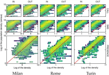
We find that such a power relationship holds in our ref-erence scenarios as well. Figure 2 portrays heat-maps of the correspondence between the ground-truth population
Milan Rome Turin
Fig. 2: ISTAT census population density versus density of calls, texts, and subscriber presence, in Milan, Rome, Turin. TABLE 1: Correlation coefficients between activity density of different types of mobile network metadata and the population census density, computed on aggregated data.
Calls Texts
In Out In Out Internet Presence
MILAN 0.684 0.679 0.715 0.727 0.757 0.791
ROME 0.805 0.800 0.835 0.860 0.882 0.912
TURIN 0.808 0.809 0.840 0.849 0.865 0.905
density and the network activity density, as recorded in each cell over the whole data collection period. The plots refer to different cities and different classes of mobile network meta-data, i.e., incoming and outgoing calls and text messages, as well as presence. All trends are clearly linear on a log-log scale: this implies that log pρiq “ logpαq ` βlog pσiq, which
is a simple transformation of (2).
Our baseline population estimation model is thus de-scribed by the expression in (2). By transforming the for-mula to a logarithmic scale as done above, we can use a linear regression model to estimate the parameters α and β. Unfortunately, all linear relationships in Figure 2 are characterized by a significant amount of noise, caused by the heterogeneity and heteroscedasticity of voice calls, text messages and subscriber presence density with respect to the actual population density. Classical linear regression models assume absence of heteroscedasticity: running a regression directly on the raw metadata would yield poor results. In order to de-noise the metadata, we take a number of actions, which are discussed in the rest of the section.
3.1 Metadata class filtering
As a first step, we determine which type of mobile network metadata is the most suitable to population estimation. To this end, we investigate the correlation between the pop-ulation census data and the different classes of metadata presented in Section 2.1, as measured in each geographical cell over time and using the full two-month data. Results are summarized in Table 1, which reports the Pearson cor-relation coefficient computed in the case of incoming and outgoing voice calls, incoming and outgoing text messages, Internet sessions, and presence. It is apparent that the pres-ence is steadily better correlated than all other metadata,
with coefficients of 0.79–0.91 that improve by 3.5%–5% the runner-up value associated with Internet session volumes.
We further examine the higher suitability of presence density as a proxy of population density in Figure 3. The top plots detail the typical daily fluctuation of the Pearson correlation coefficient, computed on 24 hourly aggregates of the two-month data. In addition to presence, the plots illustrate the correlation dynamics for incoming voice calls and text messages, as a benchmark1. The results highlight
that subscriber presence is sensibly better correlated with the ground-truth data, at all times and across all scenarios.
Interestingly, our results are aligned with those in [14], which, however, only considered calls and messages, and not the subscriber presence. In fact, their conclusion that calls between 10 am and 11 am yield the strongest correla-tion with populacorrela-tion density, is superseded by our observa-tion that subscriber presence is a much more relevant metric. In the light of these considerations, we select the subscriber presence as the mobile network metadata on top of which we develop our methodology.
3.2 Time filtering
A second dimension for filtering is time. As already ob-served in previous works, the correlation between mobile network metadata and population varies over time [13]. This effect is also present in our case studies, as shown by the bottom plots in Figure 3: they detail the variability of the correlation coefficient for subscriber presence, over daytime and in the three reference urban scenarios.
The correlation coefficient has similar dynamics in all cities, and always peaks at night. The intuitive explanation is that the ISTAT census data refers to the static popula-tion density, and residents are more frequently at home overnight. This result allows selecting a single time filter that maximizes the correlation with the ground truth for all scenarios. Hereafter, and for the purpose of training our model, we will consider σiin (2) as the subscriber presence
density in cell i during the interval between 4 am and 5 am.
3.3 Day filtering
As mentioned in Section 2.1, the mobile network metadata we employ covers 60 days in March and April 2015. An interesting question is if all these days should be considered in the regression model, or if there exists a more meaningful subset of days. Indeed, mobile network metadata is clearly affected by the diverse activity patterns and social phenom-ena that may characterize different days.
The three top plots in Figure 4 show the Pearson cor-relation coefficient in the reference cities over April2. They
refer to incoming voice calls (A), incoming text messages (B), and subscriber presence (C); according to the previous discussion, they are computed over the 4 am to 5 am interval. We still include calls and messages in order to check if they show correlation peaks on a daily basis that we could not observe in previous plots. This is not the case: the presence correlation coefficient ranges between 0.9 and 0.94, i.e., steadily higher values than those of calls and texts, lying
1. Outgoing calls and messages, and Internet sessions produced results equivalent to or worse than those obtained with incoming calls and messages. They are not shown here for the sake of clarity.
0.0 0.3 0.6
0.9 presence callin smsin
00:00 08:00 12:00 16:00 23:00 0.65 0.75 0.85 Milan 0.0 0.5
1.0 presence callin smsin
00:00 08:00 12:00 16:00 23:00 0.75 0.85 0.95 Rome 0.4 0.7
1.0 presence callin smsin
00:00 08:00 12:00 16:00 23:00
0.60 0.75 0.90
Turin
Fig. 3: Top: correlation between activity density of different types of mobile network metadata and the population census density, on a hourly basis. Bottom: zoom on presence metadata. Plots refer to Milan, Rome, Turin.
0.6 0.7
0.8 week day weekend holiday 0.6 0.7 0.8 0.6 0.8 1.0 0 2 4 6 8 91 100 110 120 0.0 0.5 1.0
Day of the year
A vg call dens . Presence SmsIn CallIn % Missing cell A B C D E Milan Rome 0.6 0.8
1.0 week day weekend holiday 0.6 0.8 1.0 0.6 0.8 1.0 0 2 4 6 8 91 100 110 120 0.0 0.5 1.0
Day of the year
A vg call dens . Presence SmsIn CallIn % Missing cell A B C D E Turin
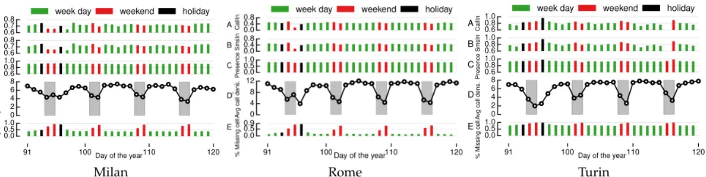
Fig. 4: Time dynamics of Milan, Rome and Turin metadata recorded between 4 am and 5 am in April 2015. A-C) Pearson correlation coefficient for incoming voice calls, incoming text messages, and subscriber presence. D) Average call density, with weekends highlighted. E) Percentage of cells with no subscriber presence metadata. Figure best viewed in colors. between 0.6 and 0.8. We confirm that subscriber presence is
a most convenient proxy of population distribution. When it comes to filtering based on days, however, no clear trend is observed in the top three plots, for all metadata types.
A more insightful result in this sense is obtained by considering the percentage of cells for which no subscriber presence metadata is available between 4 am and 5 am on each day (E). Here, a remarkable weekly pattern emerges: high peaks of missing information appear on weekends (de-noted by red bars) and holidays (de(de-noted by black bars, and corresponding to Good Friday and Easter), and reach up to 90% of cells. In order to understand why this happens, let us consider the average call density (D), i.e., the mean number of (incoming and outgoing) calls3 normalized by the cell
surface and computed over all cells during each 15-minute slot between 4 am and 5 am: here, weekdays and weekends (highlighted in gray) yield remarkably different and lower density. Such a reduced communication activity leads to seldom updated presence metadata that easily misses user occupancy in less populated cells; therefore, it increases the number of low-presence cells, which are then removed from the dataset by the operator during sanitization to mitigate privacy risks4 [17]. We conclude that a substantially lower
activity of users during non-working days is the cause for the notable absence of presence metadata on those days.
In the light of these considerations, the high correlation between presence metadata and population census during weekends and holidays (C) is ostensible, as it only concerns cells for which metadata is available. For the (many) other
3. Similar results were obtained with equivalent text message density and Internet session density, and are omitted for the sake of brevity.
4. The rationale for the operator’s choice is that if too few users are present in a cell, they may be tracked and re-identified in the metadata.
cells, the correlation cannot be computed due to the lack of presence metadata. Since working with inconsistent tem-poral supports for different cells may introduce biases in the analysis, we ultimately opt for excluding weekends and holidays from the data used to derive our model.
3.4 Outlier cell filtering
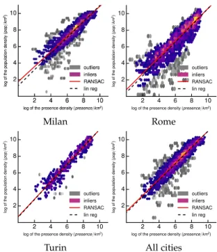
In order to estimate the parameters α and β in (2), we employ the RANSAC regressor [20] on the filtered sub-scriber presence metadata. In addition to estimating the model parameters in an iterative manner, RANSAC also automatically detects outlying points and excludes them from the regression. Figure 5 depicts heatmaps of the filtered subscriber presence metadata versus the census population density data, for the three reference scenarios of Milan, Rome and Turin separately, as well as when the data for all these cities is considered at once. A first important observation is the effect of the proposed filters. The noise is sensibly reduced with respect to the raw subscriber presence metadata, in Figure 2: most points are tagged as inliers (colored dots) by RANSAC, and follow a clear linear trend.
Still, there exists a minority of outliers (gray dots) de-tected by RANSAC. A closer look at these outliers reveals that they refer to a same subset of cells, consistently over time. Thus, those cells yield some features that make the subscriber presence recorded there less related to the local amount of population. Maps of such cells are in Figure 6.
We do not have strong evidence of why a limited number of specific cells show outlying behaviors with respect to the model. However, we speculate that two factors may contribute to this phenomenon. The first is a border effect: in all three cities, many outlying cells are located at the bound-aries of the considered geographical region. We argue that
Milan
2 4 6 8 10
log of the presence density (presence/km2)
2 4 6 8 10 log of the population density (pop /km 2) outliers inliers RANSAC lin reg Rome 2 4 6 8 10
log of the presence density (presence/km2)
2 4 6 8 10 log of the population density (pop /km 2) outliers inliers RANSAC lin reg Turin 2 4 6 8 10
log of the presence density (presence/km2)
2 4 6 8 10 log of the population density (pop /km 2) outliers inliers RANSAC lin reg All cities
Fig. 5: RANSAC regression on filtered subscriber presence metadata, in Milan, Rome, Turin, and combined scenarios.
Fig. 6: Milan, Rome, Turin. Geographical positions of the cells that determine frequent outliers detected by RANSAC. the mobile network antennas in such cells probably cover areas (and populations) beyond the limits of the scenario, and the metadata reflects that. As a result, the subscriber presence associated to frontier cells also refers to users located outside the cells, which leads to an overestimation of the population by the model.
The second factor is the temporal mismatch between our datasets. The ISTAT census dates back to 2011, whereas the mobile network metadata refers to 2015. It is not unlikely that the distribution of the population density in several ar-eas of the cities changed during the four years that separate the datasets. Figure 6 seems to corroborate this hypothesis, since many outlying cells are located in suburban areas where resident population dynamics are more subject to evolve. If this were the case, mobile network metadata may thus help updating population distribution maps at a much higher frequency than traditional survey-based methods.
In summary, however, there is a risk that outlying cells may be affected by artifacts of the spatial tessellation or by potential issues in the associated ground-truth data; we thus deem safer to filter them out when training our model.
4
M
ODEL EVALUATIONThe regression returns fitted parameters ˆα and ˆβ of (2). Our model estimates the static population density ˆρi in spatial
cell i from the filtered subscriber presence density σias
ˆ ρi“ ˆα σ
ˆ β
i. (3)
Figure 5 illustrates the curves obtained with the model (solid red lines), as well as with a pure linear fitting where β=1 (dashed black lines). The two lines are close in all plots, which underscores the quasi-linearity of the relation between subscriber presence and population in all urban scenarios: e.g., we find ˆβ=1.02 when all cities are used jointly.
4.1 Metrics
In order to assess the accuracy of the model in (3), we com-pute the determination coefficient (R2), and the Normalized Root Mean Square Error (N RM SE) of the estimates, when compared to the ground-truth data. The R2coefficient is
R2 “ 1 ´ řN i“1pρi´ ˆρiq 2 řN i“1pρi´ ¯ρq 2, (4)
where N denotes the number of cells in the spatial tessel-lation, and ¯ρ is the average population density in all cells from ground-truth data. We compute two versions of the N RM SE, which facilitates the comparison of the model results in different contexts. They are defined as
N RM SEp1q “ 1 ρmax´ ρmin d řN i“1p ˆρi´ ρiq2 N , (5) and N RM SEp2q “ 1 ¯ ρ d řN i“1p ˆρi´ ρiq2 N , (6)
where ρmaxand ρminare the maximum and minimum
pop-ulation densities in cells within the target urban scenario, as indicated by the ground truth. In the following, we will use N RM SE to refer to both expressions (5) and (6) at once.
We stress that our performance metrics are computed on all cells, including those excluded from model training.
4.2 Milan case study
We first focus on the Milan scenario. We adopt a three-fold cross-validation procedure, by separating the subscriber presence data into three equally-sized subsets in time. Two subsets are used as a training set to learn the model pa-rameters, and the third is employed as a test set to evaluate the model quality. The process is repeated three times, by changing the test subset at each iteration.
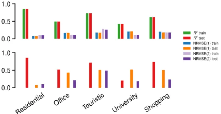
The baseline result for the Milan case study is shown in Figure 7. The top plot reports the values of the R2 and
N RM SE metrics computed on the test set, as well as on the training set for completeness. The results are separated per land use: i.e., the model is independently trained and tested on mobile network cells characterized by different land uses, extracted from the mobile network metadata as per Section 2.3. We remark that both R2and N RM SE: (i) yield comparable values for all pairs of training and test data; (ii) undergo significant variability across land uses. The first result proves that the model can correctly estimate unknown population densities from subscriber presence metadata. The second highlights how land use affects the activities of individuals, including their mobile communication habits; in turn, this diversity influences the accuracy of population estimates from mobile network metadata.
The estimation is better in residential areas, where R2=0.85, N RM SEp1q=0.075 and N RM SEp2q=0.122. This
0.0 0.5 1.0 R2train R2test NRMSE(1) train NRMSE(1) test NRMSE(2) train NRMSE(2) test Residential
Office Touristic
University Shopping 0.0
0.5 1.0
Fig. 7: Milan. Top: R2 and N RM SE for training and test
sets, separated by land use. Bottom: R2and N RM SE of the model trained on residential land use on other land uses. is a reasonable result, given that the distribution of dwelling units in the ISTAT census population is best captured in neighborhoods where households prevail. The quality of the estimation is still good (R2 above 0.6) for touristic and
shopping zones, fair (R2 close to 0.5) for office areas, and bad (R2 below 0.4) for university areas. Our speculation
is that different percentages of individuals present in these areas overnight are not resident inhabitants in the census data (but, e.g. tourists, students, or locals hanging out), hence do not appear in the population ground truth.
In the light of these considerations, the model parame-ters estimated in residential areas have the highest chance to be those actually linking population and presence metadata. We verify to what extent a model trained in residential zones can estimate populations in areas characterized by different land uses in the bottom plot of Figure 7. In the Milan case study, this approach does not degrade performance significantly, with the sole exception of university areas that however represent a negligible minority of spatial cells. This lets us consider a unifying model in the remainder of our study, by training (3) on presence metadata from cells where residential land use is predominant.
4.3 Generalization to different city scenarios
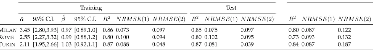
Table 2 summarizes the performance of our model in all urban scenarios. The residential portion of Table 2 refers to results obtained with data relative to cells with residential land use. It shows: (i) the model parameter values ˆα and ˆβ returned by fittings on the training set, with 95% confidence intervals; (ii) the fitting quality of the model computed over the training set, as R2 and N RM SE; (iii) the accuracy of
the estimation in the test set, as R2and N RM SE.
We remark that the values of ˆβ are consistently close to one across all of the urban scenarios we consider. Instead, ˆα tends to be city-specific5. The accuracy of the estimation is in all cases very good, attaining determination coefficients between 0.8 and 0.87, and a normalized error below 0.1.
The right portion of Table 2, under the mixed tag, outlines the performance of the model trained on residential areas, and then used to estimate the population density in the com-plete urban region, including zones that are not residential
5. We explored if a number of features (e.g., total population, average population density, conurbation size, number of cells in the geograph-ical surface, mobile network operator market share, etc.) could explain the difference, without finding significant correlations.
in nature. The accuracy remains good6, with R2in the range
between 0.76 and 0.82, and N RM SE around 0.1.
As a final test, we explore the possibility of estimating the population density in an urban area using a model trained on data collected in another city. The rationale is that, in Table 2, the ˆβ values are almost identical for all cities, and ˆα values are not dramatically different. Table 3 summarizes the estimation accuracy on all possible combi-nations of our three reference city scenarios, for both R2 and N RM SE. The pi, jq-th element in the table maps to the accuracy of a model trained on metadata and ground truth from city i, and used to estimate the population in city j.
The metric values stay fairly high (in the range 0.64-0.84) for R2 and low (between 0.1 and 0.2) for N RM SE,
in all combinations of cities, which suggests that a cross-city estimation of population density is in fact possible. This result has important practical implications, since it paves the road to the estimation of populations in cities using mobile network metadata, and without any need for training on ground-truth data on a specific urban region.
As a concluding remark, we underscore that all results above hold for our three reference cities, and we cannot claim generality beyond these. Yet, the strong consistence of model performance and the possibility of cross-city esti-mation are especially encouraging when considering that the target cities have fairly diverse topological features and population sizes, at approximately 2,850,000 (Milan), 1,350,000 (Rome) and 800,000 (Turin) inhabitants.
5
D
YNAMIC POPULATION ESTIMATIONAn interesting possibility offered by mobile network meta-data is the estimation of dynamic populations, i.e., the instantaneous distribution of city inhabitants over time, as determined by their daily activities. In this case, we do not target the evaluation of the static density of dwelling units ρi in cell i, but that of the time-varying real-time density
ρiptqin cell i, at any time t. Estimating dynamic population
densities is more challenging than approximating the static distribution of dwelling units, due to the much shorter timescale of people movements (minutes) compared to that of domicile variation (years).
The main problem in estimating dynamic populations is the lack of ground-truth data, which makes training super-vised models such as that in (3) impossible. Simply reusing the parameters ˆα and ˆβ computed for the static population is inaccurate, because those values describe the relationship between a specific subscriber presence σi and the static
density of residents: there is no certainty that the correspon-dence remains valid when inhabitants are not at home. For instance, the reduced correlation between census population information and mobile subscriber presence during working hours, in Figure 2, already advises against using parameters trained over night hours to estimate whole-day population densities at any time t.
Our approach roots instead in a novel multivariate re-lationship between the population density, the subscriber
6. We remark that these values are aligned with or better than those of current state-of-the-art solutions for static population density
estimation. For instance,R2of 0.66 and 0.8 reported in [14] and in [15],
respectively; also, theN RM SEis measured at 1.0 in [15]. A complete
TABLE 2: Model parameters and accuracy in Milan, Rome, and Turin.
RESIDENTIAL MIXED
Training Test
ˆ
α 95%C.I. βˆ 95%C.I. R2 N RM SEp1q N RM SEp2q R2 N RM SEp1q N RM SEp2q R2 N RM SEp1q N RM SEp2q
MILAN 3.45 [2.80,3.93] 0.97 [0.89,1.0] 0.86 0.073 0.097 0.85 0.075 0.097 0.80 0.087 0.122
ROME 2.55 [2.27,3.32] 0.99 [0.88,1.2] 0.80 0.100 0.094 0.80 0.102 0.095 0.73 0.093 0.132
TURIN 2.11 [1.95,2.66] 1.03 [0.92,1.1] 0.87 0.088 0.048 0.87 0.081 0.039 0.84 0.087 0.187
TABLE 3: Models trained on data of cities on rows are used to estimate the population density of cities on columns.
MIXEDLANDUSE
R2 N RM SEp1q N RM SEp2q
Milan Rome Turin Milan Rome Turin Milan Rome Turin
MILAN 0.80 0.67 0.84 0.087 0.102 0.088 0.122 0.143 0.186
ROME 0.82 0.73 0.78 0.083 0.093 0.103 0.121 0.132 0.179
TURIN 0.77 0.64 0.84 0.094 0.108 0.087 0.124 0.139 0.187
presence and the level of mobile communication activity of subscribers. This allows taking the constants α and β out of the equation, and finding a unifying expression that can be used to estimate dynamic urban populations in absence of ground-truth information.
5.1 Subscriber presence and activity levels
We start by discussing the interplay between the time-varying subscriber presence σiptqand the subscriber activity
level. The latter is the frequency at which a subscriber interacts with the mobile network. Formally, we define the activity levels for voice calls λcall
i ptq and text messages
λsms
i ptqat network cell i and time t as:
λcalli ptq “ V callin i ptq `Vicalloutptq σiptq (7) λsms i ptq “ V smsin i ptq `Vismsoutptq σiptq , (8) whereV‹
iptqstands for the number of mobile
communica-tion events of type ‹ (i.e., incoming or outgoing voice calls, incoming or outgoing text messages) recorded in mobile network cell i at time t. The subscriber presence σiptq is
a proxy of the number of “unique users”, as it provides an approximate tally of the mobile devices based on their interactions with the mobile network: the fractions in (7) and (8) respectively denote the mean number of calling and texting events per user in cell i at time t.
We can now introduce the average activity levels as λcallptq “ 1 N N ÿ i“0 λcall i ptq (9) λsmsptq “ 1 N N ÿ i“0 λsms i ptq, (10)
where N denotes the number of mobile network cells in the target geographical region. Then, λcallptq and λsmsptq
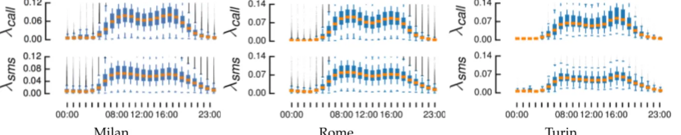
express the average number of calls and messages sent or received at time t by a user located in the whole urban areas. These activity levels are not uniform over time. Figure 8 depicts the fluctuation of λcallptq and λsmsptq in the
res-idential areas of Milan, Rome and Turin, over a day. The
error bars indicate the average and 5th, 25th, 75th and 95th
percentiles of the activity levels, on a hourly basis. For all cities, λcallptq and λsmsptqundergo major variations, with
minima at night and higher activity during work hours. This behavior is consistent across land uses, as shown in Figure 9 for the specific case of Milan. Minor variations exist, in accordance to the prevalent activities in each land land use: university and shopping areas show higher mobile communication during rush hours, and almost no network usage at night; touristic and office areas have activity peaks in the morning that then degrade until midnight. Still, the overall heterogeneity of λcallptq and λsmsptq is the same
for all land uses: Figure 10 highlights such uniformity, by aggregating the daily behavior into a single error bar for each land use. In all cases, the 75-th and 95-th percentiles of both voice calls and text messages are approximately 50% and 300% higher than the mean activity level.
Our key point here is that the heterogeneity of λcallptq
and λsmsptqin time has an impact on the correctness of the
subscriber presence information. As an illustrative example, let us consider again Figure 1: the more often a mobile device issues and receives voice calls or text messages, the more accurate is its localization in the presence data. A legitimate question is then whether the different activity levels we observe in all our urban scenarios can be linked to the model parameterization, and explain the diversity of ˆα and ˆβ noted in Section 4. We explore this possibility next.
5.2 Population estimation with activity levels
We do not have access to the real values of the parameters in (2), but to their estimations ˆα and ˆβ. We thus collect data in all cities that refer to the overnight period, i.e., from midnight to 8 am: in this period the ISTAT census infor-mation can be still considered a reliable ground truth, as most people are at home. We then draw a scatterplot of the activity levels λcallptqand λsmsptq, with the corresponding
ˆ
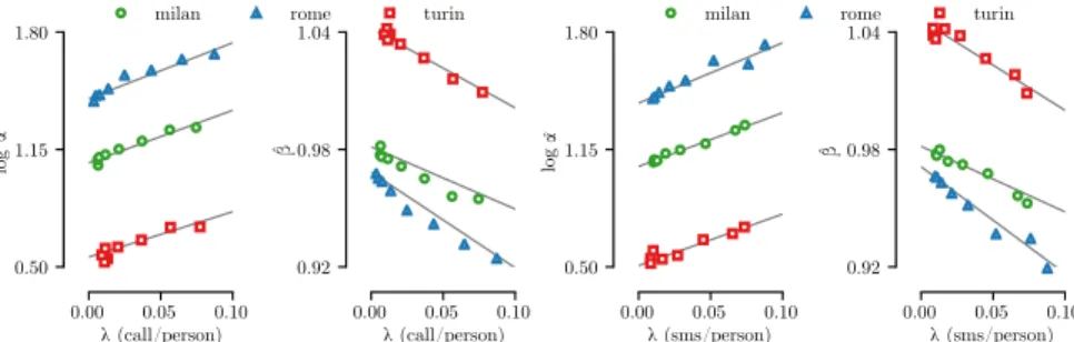
α and ˆβ obtained with the RANSAC regression model. The results for the three cities are depicted in Figure 11, and outline a striking linear relationship between the activ-ity levels and both model parameters, for all cities. Specifi-cally, ˆα grows linearly with the activity levels, while ˆβ drops linearly with the same measures. We can then re-write the parameters ˆα and ˆβ as
ˆ
α “ ˆaαλ‹ptq ` ˆbα (11)
ˆ
β “ ˆaβλ‹ptq ` ˆbβ, (12)
where ‹ denotes the type of event (i.e., calls or texts). The exact values of ˆaα, ˆbα, ˆaβ, and ˆbβare listed in Table 4.
In both (11) and (12), we observe some heterogeneity across cities. Specifically, the derivatives of the curves are quite close to each other, whereas a constant offset tells apart
Milan Rome Turin
Fig. 8: Milan, Rome, Turin. Daily activity level of mobile subscribers in residential areas, for calls (top) and texts (bottom).
Touristic University
Office Shopping
Fig. 9: Milan. Daily activity level of mobile subscribers in different land-use areas for calls (top) and texts (bottom).
resident ial office comm uting shopp ing night-lif e university 0.0 0.1 0.2 λsms (sms /pe rs on ) resident ial office comm uting shopp ing night-lif e university 0.0 0.1 0.2 λca ll (c all /pe rs on )
Fig. 10: Milan. Aggregate activity level of mobile subscribers in different land use areas for calls (left) and texts (right). the linear behavior observed in different urban areas. Such a diversity in the parameter settings evidences the need for a per-city calibration of the model. Instead, there is no significant difference between the values obtained when considering voice call or text message activity: hereinafter, we will consider the former only.
We leverage the results above to draw a unifying mul-tivariate model that links the population density to both the subscriber presence and the subscriber activity level. Specifically, we refine our estimation model as
ˆ
ρiptq “ epˆaαλiptq`ˆbαq¨ σiptqpˆaβλiptq`ˆbβq, (13)
where λiptqis a simplified notation for λcalli ptq.
The following important considerations are in order. First, the expression in (13) employs variables σiptq and
λiptqthat can be computed from mobile network metadata
at any time t. Second, unlike the original ˆα and ˆβ in (2), the new parameters ˆaα, ˆbα, ˆaβ, and ˆbβ can be regarded
as time-invariant, assuming that the linear relationships in (11) and (12) hold for any activity level. When considered jointly, these observations imply that the model in (13) is
suitable for the dynamic estimation of population densities in practical cases where ground-truth information on the instantaneous distribution of inhabitants is unavailable.
5.3 Properties of the multivariate model
We explore the basic properties of the multivariate model in Figure 12. The plot illustrates how expression (13) reshapes the relationship between the presence density and the esti-mated population density depending on the activity level λ, in the exemplary Milan scenario. The dashed line in the figure is the conceptual curve that would link the estimated population ˆρiptqto the presence σiptqif the latter metadata
reported the exact number of customers in region i. In that case, the population could be obtained by simply scaling the presence by the market share M of the mobile operator7, i.e.,
ˆ
ρiptq “M1 ¨ σiptq.
We observe that the model always lies below such a conceptual curve, compensating for the effect that the presence metadata computed with current activity levels tends to overestimate the population density. However, as the value of λ grows from 0.01 to 0.20 (the two extreme values observed in our datasets), the model approaches the ideal ˆρiptq “ M1 ¨ σiptq relationship. This is consistent
with the intuition that higher subscriber activity results in presence metadata that approximates more accurately the actual number of people present in a cell. Interestingly, such a correspondence occurs faster for low-density cells (e.g., presence is an excellent proxy for population densities below 50 individuals/km2 already at λ “ 0.14); instead,
high-density cells require subscriber presence values that are never attained in our data. At the maximum activity level recorded in our metadata, i.e., λ “ 0.20, the model is nearly equivalent to the perfectly proportional representa-tion for presence densities up to 400 devices/km2.
Finally, we comment on the suitability of the model for real-time estimation of dynamic population densities. Our multivariate model has a close form, presented in (13). Therefore, the computational complexity of the model corresponds to that of computing the equation – an op-eration performed in nanoseconds by any low-end CPU. As a result, the complexity of the model easily meets the requirements of any real-time application. Instead, the ac-tual system latency would depend from the time needed by the mobile network operator to collect and process the data required to compute the presence metadata and the activity level: however, these aspects concern the overall mobile network architecture, and are well beyond the scope of our contribution.
7. TIM, our mobile network metadata provider, has a market share of
log 0.00 0.05 0.10 λ (call/person) 0.50 1.15 1.80 ˆα
milan rome turin
0.00 0.05 0.10 λ (call/person) 0.92 0.98 1.04 ˆ β 0.00 0.05 0.10 λ (sms/person) 0.50 1.15 1.80 ˆα
milan rome turin
0.00 0.05 0.10 λ (sms/person) 0.92 0.98 1.04 ˆ β log
Fig. 11: Milan, Rome, Turin. Linear relationships between the activity level λcall
(left) and λsms(right), and the population density model parameters ˆα and ˆβ.
TABLE 4: Milan, Rome, Turin. Param-eters of the multivariate model in (13) inferred from call and text activity.
Voice calls Text messages
——Milan Rome Turin Milan Rome Turin
ˆ aα 2.90 3.15 2.34 2.91 3.11 2.64 ˆ bα 1.07 1.42 0.55 1.05 1.40 0.52 ˆ aβ -0.30 -0.50 -0.44 -0.35 -0.48 -0.43 ˆ bβ 0.98 0.96 1.04 0.98 0.97 1.04 0 500 1000 1500 2000
presence density (devices/km2)
0 2000 4000 6000 population density (individuals /km 2) λ=0.01 λ=0.03 λ=0.05 λ=0.07 λ=0.09 λ=0.12 λ=0.14 λ=0.16 λ=0.18 λ=0.20 ρ=1 Mσ Fig. 12: Milan. Dynamic population density estimated by the multivariate model as a function of presence, for different values of the activity level. The dashed line depicts the perfectly proportional relationship ρiptq “M1 ¨ σiptq.
6
C
ASE STUDIESIn this section, we provide proof-of-concept exploitations of the model in (13). Specifically, we first leverage the model to provide a glance of the population dynamics during typical days in Milan and Turin. Then, we assess the model capac-ity to approximate the population denscapac-ity during special events, such as sport matches and public rallies.
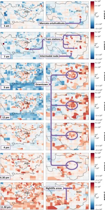
6.1 A day in the life of Milan
Figure 13 illustrates the dynamic distribution of the pop-ulation in Milan and its suburbs, as inferred from our multivariate model, during key times of one normal day, i.e., Monday April 13, 2015. Left plots refer to the whole conurbation, whereas right plots focus on the actual city. In each plot, colors denote the z-score, which measures the deviation from the mean of the population distribution at each location. Formally, the z-score in cell i at time t is
ziptq “
ˆ
ρiptq ´ µi
δi
, (14)
where µi and δi are the mean and standard deviation of
the population density at cell i, computed over the values estimated by our model during the full two months, i.e., over ˆρiptq @t. As a result, the plots show how the population
density fluctuates at specific times: variations range from high in-flow of individuals moving into a cell (red) to high out-flow of individuals leaving a cell (blue), passing by neutral cells where the population density does not vary during the observation period (white).
Reasonable dynamics emerge from the plots. At 5 am, the only point of interest showing relevant activity is the mercato ortofrutticolo, i.e., the wholesale produce market of Milan. The market attracts farmers and merchants very
early in the morning, as highlighted by the red spot in the top right plot. At 7 pm, the population density is espe-cially high around main transportation hubs, such as train stations and intermodal exchange nodes. The population density grows significantly in the city center throughout the morning, see e.g., the plots at 9 am and 12 pm. At the same times, the suburban and rural areas show low z-scores, indicating a clear in-flow of inhabitants from around the city to downtown, where office areas are located. The trend is then reversed in the afternoon, starting at 4 pm and more clearly at 6.30 pm, when people leave from the office. Here, the city center tends to become less populated, with an out-flow of inhabitants towards the city outskirts. Finally, it is interesting to observe that late at night, at 11.30 pm, the population is mostly at home, with high z-scores in suburban and rural areas, or in nightlife areas.
Overall, the results in Figure 13 show that our multivari-ate model can capture sensible dynamics of the population density at an intra-urban scale.
6.2 Crowds at large-scale events
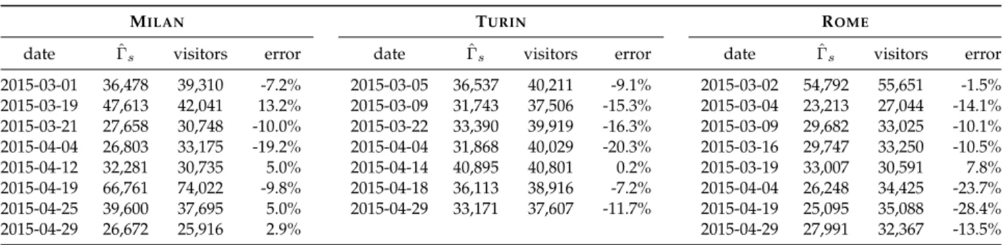
Our proposed model does not only capture typical dynam-ics of the urban population density, but can also estimate crowds at major social events. Interestingly, official figures about attendance at such events offer an original means to validate our assumptions on the time-invariance of the parameters in Table 4, as well as the overall quality of the estimates returned by our multivariate model.
6.2.1 Football matches
Football matches are traditionally very popular events throughout Italy. Figure 14 highlights the population den-sity in Milan and Turin during games of major local football teams. For the Milan case, the plot refers to April 19, a Sunday, at 10 pm. The model conveys well the crowd attracted by an important football match between AC Milan and Inter Milan, the two city teams, that took place on that day at San Siro, the main city stadium. The stadium position is even more evident in the case of Turin, on April 14 at 9 pm. At that time, the local team, Juventus FC, was playing a quarter-final Champions League game against AS Monaco.
In fact, the multivariate model allows going beyond a simple visualization of population density peaks in and around the stadiums during matches. By leveraging the expression in (13), we can produce actual estimates of the attendance at matches through the following steps.
‚ We identify the mobile network cells that provide
TABLE 5: Comparative evaluation of estimated and actual attendance at football matches in Milan, Turin and Rome.
MILAN TURIN ROME
date Γˆs visitors error date ˆΓs visitors error date Γˆs visitors error
2015-03-01 36,478 39,310 -7.2% 2015-03-05 36,537 40,211 -9.1% 2015-03-02 54,792 55,651 -1.5% 2015-03-19 47,613 42,041 13.2% 2015-03-09 31,743 37,506 -15.3% 2015-03-04 23,213 27,044 -14.1% 2015-03-21 27,658 30,748 -10.0% 2015-03-22 33,390 39,919 -16.3% 2015-03-09 29,682 33,025 -10.1% 2015-04-04 26,803 33,175 -19.2% 2015-04-04 31,868 40,029 -20.3% 2015-03-16 29,747 33,250 -10.5% 2015-04-12 32,281 30,735 5.0% 2015-04-14 40,895 40,801 0.2% 2015-03-19 33,007 30,591 7.8% 2015-04-19 66,761 74,022 -9.8% 2015-04-18 36,113 38,916 -7.2% 2015-04-04 26,248 34,425 -23.7% 2015-04-25 39,600 37,695 5.0% 2015-04-29 33,171 37,607 -11.7% 2015-04-19 25,095 35,088 -28.4% 2015-04-29 26,672 25,916 2.9% 2015-04-29 27,991 32,367 -13.5%
exact maps of the signal propagation and antenna cov-erage areas are not available, we tend to be inclusive, considering all cells that intersect with the stadium surface, as well as the adjacent ones.
‚ For each cell i PN , we determine the presence density
in a normal situation, i.e., when no match is played at the stadium. To that end, we record all presence density values at the same weekday and time of the match, excluding those days where another match was played; we then compute the median of such presence densities, and denote the result as ¯σiptq.
‚ We establish the time of the match at which the
pres-ence density across all cells inN reaches its peak, i.e., tpeak“ arg max
tPT
ÿ
iPN
σiptq, (15)
whereT is the match timespan, from 15 minutes before kickoff to 15 minutes after the final whistle.
‚ We compute the average presence density in normal
conditions, σnorm, and during the match, σmatch, as
σnorm “ ÿ iPN Ai ř jPNAj ¨ ¯σiptpeakq (16) σmatch “ ÿ iPN Ai ř jPNAj ¨ σiptpeakq, (17)
where Ai indicates the surface of mobile network cell
i. We opt for an average weighted on the relative cell sizes, so as to account for the fact that the cells in N may have quite diverse surfaces.
‚ We calculate the mean activity level in all concerned
cells during the course of match as r λ “ 1 |N | ÿ iPN λiptpeakq, (18)
where operator | ¨ | designates the cardinality of a set. Here, a simple arithmetic mean suffices, since the λiptpeakqvalues are averaged over users and unrelated
to cell surfaces.
‚ The attendance ˆΓ is finally obtained via our
multivari-ate model as ˆ Γ “ ” paαrλ ` bαqpσmatch´σnormqpaβλ`br βq ı ¨ÿ jPN Aj. (19)
The last operation above applies the model in (13) to the difference between σmatch and σnorm, i.e., to the
in-creased presence density during the football match. The result is an estimate of the population density inflation (in
attendees/km2) caused by the crowd in the stadium.
Multi-plying by the total geographical surface allows inferring the actual attendance at the event.
In order to assess the quality of the estimation, we consider all matches played in March and April 2015 by the first-division football teams of Milan, Turin and Rome, and compute their attendance ˆΓ from (19). We then compare such estimated attendance to the official figures reported by local authorities, which are very precise and represent a reliable ground-truth. The overall attendance estimation error, in terms of the metrics introduced in Section 4.1 is R2
“ 0.74 and N RM SEp1q “ 0.102: these values are aligned with those for the static population estimation, and demonstrate that our multivariate model can measure population densities in a time-varying environment with similar accuracy.
Further details are provided in Table 5, which reports the date, estimated and ground-truth attendance for each match. Overall, there is a good agreement between the values, with relative errors that range from 0.2% to 28.4%, and an average error of 11.9%. These results are especially encouraging when considering that our approach is general, and not specifically designed for large-scale events.
6.2.2 Public march
A second example of social happening detected from the dynamic population estimated by our multivariate model is a public manifestation that occurred in Milan, on Saturday April 25. On that day, Italy celebrated the 70th anniversary of liberation after World War II, and a large crowd marched along the streets of the city to commemorate the event. Figure 15 illustrates the significant increase of the z-score of the dynamic population density inferred by our model at different times during the manifestation. Namely, the plots allow appreciating the initial gathering of people in the Porta Venezia neighborhood, the two-hour procession in the city center, and the final arrival at the Duomo cathedral. This maps very well to the actual route of the parade, in the left plot of Figure 16.
Also in this case, our model can be leveraged to approx-imate the number of participants to the march. The steps are the same detailed in Section 6.2.1. Notably, we consider presence metadata in all cells that provide coverage to the path of the public march in the left plot of Figure 16, as well as their immediately adjacent cells, during the whole duration of the rally. The right plot of Figure 16 shows the results returned by the multivariate model. There are approximately 5,000 people strolling in the march area dur-ing a typical early afternoon on sprdur-ing Saturdays; however,
Mercato ortofru+colo 5 am. Train sta)ons Intermodal node 7 am. Downtown 9 am. 12 pm. 4 pm. 6.30 pm. Nightlife areas 11.30 pm.
Fig. 13: Dynamic distribution of Milan population on April 13, 2015. Top to bottom: 5 am, 7 am, 9 am, 12 pm, 4 pm, 6.30 pm, 11.30 pm. Left plots show the whole conurbation, right ones the city only. Figure best viewed in colors.
the population increases dramatically on the demonstration day. We estimate the peak attendance at 37,000 persons8, in the central phases of the march. Official and unofficial fig-ures evaluate the total number of participants at 50,000 and 60,000, respectively [21], [22]. However, our model captures the instantaneous number of participants, and not the total one: as this is a four-hour demonstration, we speculate that the discrepancy between the official figures and our estimate is explained by a natural turnover of attendees, some of which conclude the march and leaving the manifestation before others join it at its start location.
8. This value represents the increased presence over the normal population, as in the case of football matches.
San Siro stadium
Juventus stadium
Fig. 14: Examples of dynamic distribution of populations during football matches in Milano, on April 19 at 10 pm (left), and in Turin, on April 14 at 9 pm (right).
Porta Venezia
Duomo
1 pm 2 pm
3 pm 4 pm
Fig. 15: Dynamic distribution of population during a public march in Milan on April 25. Z-scores of the estimated population densities from 1 pm to 4 pm.
7
C
OMPARATIVE EVALUATIONWe carry out a comparative performance evaluation in order to clearly position our approach with respect to previously proposed competitor solutions. Specifically, the current state-of-the-art techniques for the estimation of pop-ulation densities from mobile network metadata are those presented in [14] and [15]. The former targets static popu-lation distribution estimation, while the second is designed for dynamic population density estimation. Therefore, we compare our multivariate model with the solution in [14] in the static case, and with that in [15] in the dynamic case.
7.1 Static population
The approach in [14] performs a random forest regression on a large number of per-cell features that include the hourly volumes of incoming and outgoing calls and text messages, the hourly volume of Internet sessions, and the surface fraction belonging to each land use. Land uses are classified into buildings, vegetation, water, road, and railroads, and obtained from the OpenStreetMap database [23] (41% of the cells) or inferred from satellite imagery (59% of the
Fig. 16: Public march in Milan on April 25, 2015. Left: path of the march (blue dashed line). Right: estimated attendance at the march, as the usual baseline population (cyan dashed line) and increase during the march (red solid line).
cells). Each feature is computed at three different scales, by considering cells in isolation as well as by aggregating neighboring cells into 3ˆ3 and 5ˆ5 grid squares.
In fact, the random forest regression is tested in one of the scenarios we also consider, i.e., the conurbation of Milan, using an equivalent dataset provided again by TIM in the context of the 2014 Big Data Challenge. Therefore, we can directly compare the accuracy in our results with that attained in [14]. In the best configuration, where only the 16 most important features are retained for training, the random forest technique presented in [14] achieves an R2of
0.66. The equivalent result obtained with our model is 0.80, as shown in Table 2 (Milan, mixed land use): this amounts to an improvement that exceeds 21%.
The better performance of our model is due to a com-bination of factors. First, we leverage subscriber presence, which is a more reliable proxy of population density than the mobile network metadata used in [14]. Second, we employ land use information that tells apart human activi-ties (e.g., residential versus office areas) rather than simple urbanization (e.g., buildings versus vegetation): therefore, our notion of land use has a more direct relationship with population distributions. Third, we filter the metadata based on daytime, land use and outlying human dynamics: in this way, we account for important phenomena, such as the heterogeneity of subscribers’ behaviors over the day and during the night, the diversity of mobile service usage in residential and non-residential area, or the variations of mobile traffic activity during weekdays and weekends or holidays. Given the rather intuitive nature of these phenom-ena, designing filters based on reasoning is more effective than having a machine learning technique guess them.
7.2 Dynamic population
The approach in [15] mimics several of our solutions, as originally presented in [24]. It leverages regressions on the power-law model of population density in (2), where it uses the number of subscribers at 7 am as the σi
vari-able: this is semantically similar, but not identical, to the subscriber presence we employ as σi. Also, the solution
in [15] performs the regression on different functional re-gions separately, which is equivalent to telling apart land uses. Functional regions are urban areas characterized by different densities of points of interest, and are classified into residence, entertainment, business, industry, education, scenery spot and suburb.
However, the model in [15] fundamentally differs from ours in two aspects.
‚ It uses separate estimators for different functional
re-gions. This corresponds to regressing a different pα, βq pair for each land use in (2). As a result, the approach in [15] hinges on an array of power-law models.
‚ It implements the estimation of the dynamic population
density via a time-varying rescaling factor Rt, which is
applied uniformly to all cells9at time t and ensures that the total population stays constant over time.
9. The study in [15] considers a spatial tessellation based on func-tional regions and not a Voronoi tessellation based on the mobile network deployment. In our case, we derive land use from mobile network metadata, hence the two tessellations match.
Xu et al Khodabandelou et al 0.0 0.2 0.4 0.6 re lat iv e err or *** Tu rin 04 /1 4 Milan 04/29 Rome 03/02 Milan 04/12 Milan 04/25 Rome 03/19 Tu rin 04 /1 8 Milan 03/01 Milan 03/21 Rome 03/09 Rome 03/16 Tu rin 03 /0 5 Rome 03/04 Rome 04/29 Tu rin 04 /2 9 Milan 03/19 Tu rin 03 /0 9 Milan 04/04 Tu rin 03 /2 2 Milan 04/19 Tu rin 04 /0 4 Rome 04/04 Rome 04/19 0.0 0.2 0.4 0.6 relativ e error Xu et al Khodabandelou et al
Fig. 17: Relative error in the estimated attendance at football matches, using the model in in [15] and our proposed mul-tivariate model. Left: results aggregated over all matches in all cities. Right: results for individual matches.
Formally, the design choices above lead to a model ˆ ρiptq “ Rt¨ ˆαfσiptq ˆ βf, where R t“ ř iρiAi ř iρˆiptqAi , (20) for each spatial cell i of functional region f at time t. In (20), ˆ
αfand ˆβfare the power-law parameters regressed from the
static population for functional region f , ρi is the
ground-truth static population in cell i, and Aiis cell i surface.
In the original work, the model in [15] is cross-validated with transport data in the region of Shanghai, PRC. The urban environment and validation methodology are very different from those we consider, hence a direct compari-son with our results is impossible. For the sake of a fair comparison, we thus implement10the solution in [15], and
evaluate its performance in our reference scenarios. The validation strategy is the same we adopted in Section 6.2.1, i.e., leveraging ground-truth attendance at football matches. Figure 17 displays the relative error of the estimation made by the solution in [15] and our proposed multivariate model. The left plot summarizes the results over all matches listed in Table 5, as the 5th, 25th, 50th, 75th and 95th
per-centiles. The relative error incurred by the approach in [15] is approximately twice that caused by our model, for all these statistics; in the median case, it exceeds a factor 2.2. The statistical validity of the comparison is confirmed by a two-sided Mann-Whitney U-test, which returns a p-value of 0.0005. When disaggregating results for all matches, in the right plot, it is evident that our estimation technique performs consistently better. A couple of outliers apart, our model attains peaks of improvement at 0.4.
Different matches can attract a very diverse number of spectators, hence we also investigate how the two models compare in terms of absolute error, i.e., the discrepancy in the number of attendees between estimates and ground truth. Figure 18 shows that the performance are aligned with those observed with relative errors: also in this case our model grants a 50% error reduction, consistently across matches. Thus, our conclusions hold also in this case.
We believe that the better accuracy achieved by our model roots in (i) its capability to capture the dependence
10. We had to make two approximations in our implementation. First, we use subscriber presence instead of the number of subscribers, as we do not have access to the latter in our scenarios. Second, we employ MWS-based land uses instead of functional regions, as we do not have access to high-detail points of interest databases in our scenarios. We argue that these are minor changes, as the replacement metadata is semantically close to that employed in [15], and the core differences between the two models lie elsewhere.
Xu et al Khodabandelou et al 0 5 10 15 20 ab so lut e err or × 10 3 *** Tu rin 04 /1 4 Milan 04/29 Rome 03/02 Milan 04/12 Milan 04/25 Rome 03/19 Tu rin 04 /1 8 Milan 03/01 Milan 03/21 Rome 03/09 Rome 03/16 Tu rin 03 /0 5 Rome 03/04 Rome 04/29 Tu rin 04 /2 9 Milan 03/19 Tu rin 03 /0 9 Milan 04/04 Tu rin 03 /2 2 Milan 04/19 Tu rin 04 /0 4 Rome 04/04 Rome 04/19 0 5 10 15 20 25 30 ab so lu te er r⇥ 10 3 Xu et al Khodabandelou et al
Fig. 18: Absolute error in the estimated attendance at foot-ball matches, using the model in in [15] and our pro-posed multivariate model. Left: results aggregated over all matches in all cities. Right: results for individual matches. of the regression parameters on the user activity levels λ, which is instead neglected by the time-invariant p ˆαf, ˆβfq
in [15], and (ii) its exclusive reliance on regression in resi-dential land uses. Concerning this second aspect, we argue that the early morning population in non-residential regions may not map well to people living in those areas; depending on the nature of the area, it rather corresponds to com-muters, early workers, tourists, etc. Therefore, a regression trained on such land uses will lead to unreliable parameters α and β. As a supporting evidence from Figure 18–17, the city with more heterogeneous land uses, i.e., Milan, is the one where the solution in [15] performs the worst.
8
R
ELATED WORKThere is wide agreement on the suitability of mobile net-work metadata as a source of information for human mo-bility analysis. Specifically to population distribution esti-mation, mobile network metadata was first proposed as a proxy for the density of inhabitants in [9]. Early evidences of the existence of an actual correlation between the mobile communication activity and the underlying population den-sity were presented in [10], by comparing city population sizes and amounts of mobile network customers.
Subsequent works carried out more comprehensive eval-uations. In [25], the home location of each subscriber was localized as the most frequently visited cell with a home profile, i.e., where the activity peaks at evening. The density of home locations was then found to match very well –with a 0.92 correlation– census data on nationwide population distribution. Similarly, an excellent agreement between the overnight spatial density of mobile subscribers and that of nationwide static populations was found in [26], [27]. However, these results refer to populations at the scale of a whole country, with a spatial granularity at the level of counties or tracts, i.e., large regions that comprise multiple cities each. Our focus is instead on urban population dis-tribution estimation within individual urban areas: down-scaling the investigation to a citywide level requires orders-of-magnitude higher accuracy, and is a harder challenge.
Citywide population estimation from mobile network metadata has been addressed by a limited number of works in the literature. In [11], voice calls, text message, and Internet activity metadata, combined with Twitter records, were found to be highly correlated with the number of people at specific city locations (i.e., sports arena and air-port) during a target time interval. In [12], LandScan™, a tool for ambient population estimation, was employed to explore the relationship between the voice call activity and
the underlying inhabitant density, at a 1-km2resolution. The
authors found a weak correlation of 0.24, later improved to 0.45 by limiting the analysis to selected time intervals rather than considering the daily communication volume. In [13], telecommunication data was mixed with a num-ber of other sources, including information on land use, road networks, satellite nightlights, and slope. By feeding such data to a asymmetric modeling approach, the authors obtained a high 0.92 correlation with census information. This solution is employed by the Worldpop initiative, which aims at building fine-grained maps of static population densities in underdeveloped countries [28]. However, the high correlation mentioned before is a nationwide average, and the authors indicate that the accuracy is lower for the most densely populated areas, i.e., large cities. Indeed, in such areas, a normalized error of around 0.6 is measured in [13], whereas we obtain values below 0.1.
The current state-of-the-art in the estimation of citywide population distribution from mobile network metadata is represented by the approaches in [14] and in [15]. Section 7 provides a thorough comparative evaluation. In addition to granting improved performance, our solution is the first that is (i) evaluated in multiple cities so as to demonstrate its gen-eral viability, and (ii) validated using attendances at sports and public events as ground-truth dynamic populations.
Finally, an earlier version of this paper focuses on static population estimation, and only briefly sketches the multi-variate model for the dynamic population estimation [24]. In addition to general presentation improvements, the present document improves the conference version by including: (i) a much sounder discussion of the multivariate model design; (ii) an original validation methodology for dynamic population estimates; (iii) a comprehensive evaluation of the model performance with respect to ground truth informa-tion and in comparison with state-of-the-art benchmarks.
9
C
ONCLUSIONSWe introduced a novel approach to the estimation of popu-lation density based on mobile network metadata, for both static and dynamic populations.
Building on the well-known power relationship between the mobile network activity density and the population density, our baseline model of static population density yields several unique properties: (i) it builds exclusively on metadata collected by mobile network operators avoiding complex and cumbersome data mixing; (ii) it leverages for the first time subscriber presence data inferred from the mobile communications of each user, which is found to be a much better proxy of the population distribution than previously adopted metrics; (iii) it introduces a number of original data filters based on time and land use that allow refining the population distribution estimates. Thanks to these features, when tested with substantial real-world metadata, our model outperforms previous proposals in the literature, allowing for a reliable representation of static populations across different cities.
In addition, we extended the baseline model to a mul-tivariate version that exploits a new time-invariant linear relationship between the power law parameters and the subscriber activity levels. The resulting multivariate model can be used to determine population densities in a dynamic