HAL Id: hal-01111155
https://hal.archives-ouvertes.fr/hal-01111155
Submitted on 29 Jun 2015
HAL is a multi-disciplinary open access
archive for the deposit and dissemination of
sci-entific research documents, whether they are
pub-lished or not. The documents may come from
teaching and research institutions in France or
abroad, or from public or private research centers.
L’archive ouverte pluridisciplinaire HAL, est
destinée au dépôt et à la diffusion de documents
scientifiques de niveau recherche, publiés ou non,
émanant des établissements d’enseignement et de
recherche français ou étrangers, des laboratoires
publics ou privés.
Conflict Equivalence of Branching Processes
David Delfieu, Maurice Comlan, Medesu Sogbohossou
To cite this version:
David Delfieu, Maurice Comlan, Medesu Sogbohossou. Conflict Equivalence of Branching Processes.
International Journal On Advances in Systems and Measurements, IARIA, 2015, 8 (1&2), pp.85-203.
�hal-01111155�
Conflict Equivalence of Branching Processes
David Delfieu, Maurice Comlan
Polytech’NantesInstitute of Research on Communications and Cybernetics of Nantes, France
Email: [email protected] [email protected]
M´ed´esu Sogbohossou
Polytechnic School of Abomey-Calavi Laboratory of Electronics, Telecommunications and Applied Computer Science, Abomey-Calavi, BeninEmail: [email protected]
Abstract—For concurrent and large systems, specification step is a crucial point. Combinatory explosion is a limit that can be encountered when a state space exploration is driven on large specification modeled with Petri nets. Considering bounded Petri nets, technics like unfolding can be a way to cope with this problem. This paper is a first attempt to present an axiomatic model to produce the set of processes of unfoldings into a canonic form. This canonic form allows to define a conflict equivalence.
Index Terms—Petri Nets; Unfolding; Branching process; Alge-bra.
I. INTRODUCTION
The complexity and the criticity of some real-time system (transportation systems, robotics), but also the fact that we can no longer tolerate failures in less critical realtime systems (smartphones, warning radar devices) enforces the use of verification and validation methods. Petri nets are a widely used tool used to model critical real-time systems. The formal validation of properties is then based on the computation of state space. But, this computation faces generally, for highly concurrent and large systems, to combinatory explosion.
The specification of parallel components is generally mod-eled by the interleavings of the behavior of each components. This semantics of interleaving is exponentially costly in the computing of the state space. Partial order semantics have been introduced to shunt those interleavings. This semantics prevents combinatory explosion by keeping parallelism in the model.
The objective of this approach is to pursue a theoretical as-pect: to speed up the identification of the branching processes of an unfolding. The notion of equivalence can be used to make a new type of reduction of unfoldings.
Finite prefixes of net unfoldings constitute a first trans-formation of the initial Petri Net (PN), where cycles have been flattened. This computation produces a process set where conflicts act as a discriminating factor. A conflict partitions a process in branching processes. An unfolding can be transformed into a set of finite branching processes. These
processes constitute a set of acyclic graphs - several graphs can be produced when the PN contains parallelism - built with events and conditions, and structured with two operators: causality and true parallelism. An interesting particularity of an unfolding is that, in spite of the loss of global marking, these processes contain enough information to reconstitute the reachable markings of the original Petri nets. In most of the cases, unfoldings are larger than the original Petri net. This is provoked essentially when values of precondition places exceed the precondition of non simple conflicts. This produces a lot of alternative conditions. In spite of that, a step has been taken forward: cycles have been broken and the conflicts have structured the nets in branching processes.
This paper proposes proposes an algebraic model for the definition and the reduction of the branching process of an unfolding. This paper extends [1] to reset Petri nets. Reset arcs are particularly useful, they bring expressiveness and compactness. In the example presented in the Section VI, reset arcs allow to clear the states particularly when the user has several attempts to enter its code.
A lot of works have been proposed to improve unfolding algorithms [2][3][4][5]. Is there another way to draw on recent works about unfolding? In spite of the eventual increase of the size of the net unfoldings, the suppression of conflicts and loops has decreased its structural complexity, allowing to compute the state space and to the extract of semantic information.
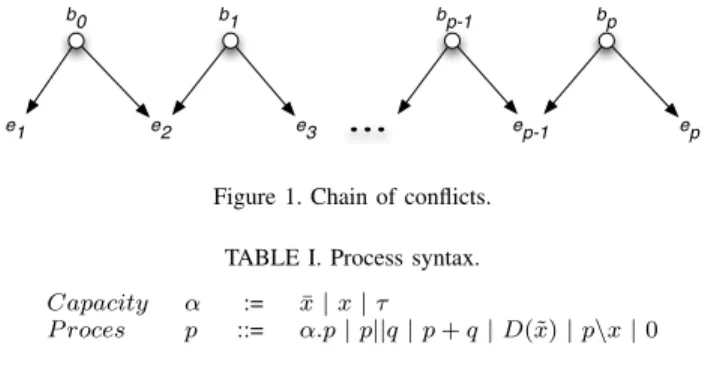
From a developer’s point of view an unfolding can be efficiently coded by a boolean table of events. This table describes every pair to pair relation between events. This table has been the starting point of our reflection: it stresses the point that a new connector can be defined to express that a set of events belong to the same process. This connector allows to aggregate all the events of a branching process. For example, a theorem is proposed to compute all the branching processes, in canonic form, for chains of conflicts of the kind illustrated in Figure 1.
e1 e2 ep-1 ep
b0 b1 bp-1 bp
e3
Figure 1. Chain of conflicts. TABLE I. Process syntax.
Capacity α := x | x | τ¯
P roces p ::= α.p | p||q | p + q | D(˜x) | p\x | 0
of combining process algebra [6][7] and Petri nets [8]. The axiomatic model of Milner’s process with Calculus of Communicating Systems (CCS) is compared with the branching processes and related to other works in Section II. Then, after a brief presentation of Petri nets and unfoldings in Section III, Section IV presents our contribution with the definition of an axiomatic framework and the description of properties. The last section presents examples, in particular, illustrating a conflict equivalence.
II. RELATEDWORK
Process algebra appeared with Milner [7] on the Calculus of Communicating Systems (CCS) and the Communicating Sequential Processes (CSP) of Hoare [6]. These approaches are not equivalent but share similar objectives. The algebra of branching process proposed in this paper is inspired by the process algebra of Milner. CCS is based on two central ideas: The notion of observability and the concept of synchronized communication; CCS is as an abstract code that corresponds to a real program whose primitives are reduced to simple send and receive on channels. The terms (or agents) are called processes with interaction capabilities that match requests communication channels. The elements of the alphabet are observable events and concurrent systems (processes). They can be specified with the use of three operators: sequence, choice, and parallelism. A main axiom of CCS is the rejection of distributivity of the sequence upon the choice. Let p and q be two processes, the complete syntax of process is described in the Table I. a b c a b c a
Figure 2. Milner: rejection of distributivity of sequence on choice.
Consider an observer. In the left automaton of Figure 2, after the occurrence of the action a, he can observe either b or c. In right automaton, the observation of a does not imply that b and c stay observable. The behavior of the two automata are not equivalent.
In CCS, Milner defines the observational equivalence. Two automata are observational equivalent if there are bisimular.
On a algebraic point of view, the distributivity of the sequence on the choice is rejected in equation (1):
a.(b + c) 6≡behaviorallya.b + a.c (1)
The key point of our approach is based on the fact that this distributivity is not rejected in occurrence nets. The timing of the choices in a process is essential [9]. The nodes of occurrence nets are events. An event is a fired transition of the underlying Petri net. In CCS, an observer observes possible futures. In occurrence nets, the observer observes arborescent past. This controversy in the theory of concurrency is an important topic of linear time versus branching time. In the model, equation (2) holds:
a ≺ (b ⊥ c) ≡ (a ≺ b) ⊥ (a ≺ c) (2)
Equation (2) is a basic axiom of our algebraic model. The equivalence relation differs then from bisimulation equiva-lence. This relation will be defined in the following with the definition of the canonic form of an unfolding.
Branching process does not fit with process algebra on numerous other aspects. For example, a difference can be noticed about parallelism. While unfolding keeps true paral-lelism, process algebra considers a parallelism of interleaving. Another difference is relative to events and conditions, which are nodes of different nature in an unfolding. Conditions and events differ in term of ancestor. Every condition is produced by at most one event ancestor (none for the condition standing for m0, the initial marking), whereas every event may have 1
or n condition ancestor(s).
In CCS, there is no distinction between conditions and events. Moreover, conditions will be consumed defining pro-cesses as set of events. However, a lot of works [5][9][10] have shown the interest of an algebraic formalization: it allows the study of connectives, the compositionally and facilitates reasoning (tools like [11]). Let have two Petri nets; it is questionable whether they are equivalent. In principle, they are equivalent if they are executed strictly in the same manner. This is obviously a too restrictive view they may have the same capabilities of interaction without having the same internal implementations. These works resulted to find matches (rather flexible and not strict) between nets. Mention may be made among other the occurrence net equivalence [12], the bisimulation equivalence [13], the partial order equivalence [14], or the ST-bisimulation equivalence [15]. These different equivalences are based either on the isomorphism between the unfolding of nets or on observable actions or traces of the execution of Petri nets or other criteria.
The approach developed in this paper proposes a new equivalence, which is weaker than a trace equivalence; it does not preserves traces but preserves conflicts. The originality of the approach is to encapsulate causality and concurrency in a new operator, which “aggregates” and “abstracts” events in a process. This new operator reduces the representation and accelerates the reduction process. This paper intends first, to give an algebraic model to an unfolding, and second,
to establish a canonic form leading to the definition of an equivalence conflict.
III. UNFOLDING APETRINET
In this section, Petri nets and unfolding of Petri nets are presented.
A. Petri Net
A Petri net [8] N =< P, T, W > is a triple with: P , a finite set of places, T , the finite set of transitions, P ∪ T are nodes of the net; (P ∩ T = ∅ signifies that P and T are disjoint), and W : (P × T ) ∪ (T × P ) → N , the flow relation defining arcs (and their valuations) between nodes of N . A marking of N is a multiset M: P → {0, 1, 2, ...} and the initial marking is denoted M0.
The pre-set (resp. post-set) of a node x is denoted •x = {y ∈ P ∪ T | W(y, x) > 0} (resp. x• = {y ∈ P ∪ T |
W(x, y) > 0}). A transition t ∈ T is said enabled by m iff: ∀p ∈•t, m(p) ≥ W(p, t). This is denoted: m→ Firing of tt
leads to the new marking m0 (m → mt 0): ∀p ∈ P, m0(p) =
m(p) − W(p, t) + W(t, p). The initial marking is denoted m0.
A Petri net is k-bounded iff ∀m, reachable from m0, m(p) ≤
k (with p ∈ P ). It is said safe when 1-bounded. Two transitions are in a structural conflict when they share at least one pre-set place; a conflict is effective when these transitions are both enabled by a same marking. The considered Petri nets in this paper are k-bounded.
Reset arcs constitute an extension of Petri nets. These arcs does not change the enabling rules of transitions [16]. If Rst(p, t) represents the set of reset arcs from a transition t to a place p. If M → Mt 0 then ∀p ∈ P such as Rst(p, t) = 0,
M0(p) = 0. But if W (t, p) > 0 then M0(p) = W (t, p). The firing rule is defined by the following relation
∀p ∈ P, M0= (M − P re(p, t)) . R(p, t) + P ost(p, t) where “.” is the Hadamard matrix product.
Definition 1 (Reset arc Petri Nets). A reset arc Petri Nets is a tuple NR=< P, T, W, R > with < P, T, W > a Petri nets
andRst : P × T → {0, 1} is the set of reset arcs (Rst(p, t) = 0 is there exists a reset arc binding p to t, else Rst(p, t) = 1).
B. Unfolding
In [3], the notion of branching process is defined as an initial part of a run of a Petri net respecting its partial order semantics and possibly including non deterministic choices (conflicts). This net is acyclic and the largest branching process of an initially marked Petri net is called the unfolding of this net. Resulting net from an unfolding is a labeled occurrence net, a Petri net whose places are called conditions (labeled with their corresponding place name in the original net) and
transitions are called events (labeled with their corresponding transition name in the original net).
An occurrence net [17] is a net O =< B, E , F > , where B is the set of conditions (places), E is the set of events (transitions), and F the flow relation (1-valued arcs), such that:
• for every b ∈ B, |•b| ≤ 1; • O is acyclic;
• for every e ∈ E, •e 6= ∅;
• O is finited preceded;
• no element of B ∪ E is in conflict with itself;
• F+, the transitive closure of F , is a strict order relation. M in(O) = {b | b ∈ B, |•b| = 0} is the minimal conditions set: the set of conditions with no ancestor can be mapped with the initial marking of the underlying Petri net. Also, M ax(O) = {x | x ∈ B ∪ E , |x•| = 0} are maximal nodes. A configuration C of an occurence net is a set of events satisfying:
• if e ∈ C then ∀e0 ≺ e implies e0 ∈ C (C is causally
closed);
• ∀e, e0∈ C : ¬(e ⊥ e0) (C is conflict-free).
A local configuration [e] of an event e is the set of event e’, such that e0 ≺ e.
Three kinds of relations could be defined between the nodes of O:
• The strict causality relation noted ≺: for x, y ∈ B ∪
E, x ≺ y if (x, y) ∈ F+ (for example e
3 ≺ e6, in
Figure 3.b).
• The conflict relation noted ⊥: ∀b ∈ B, if e1, e2 ∈ b•
(e16= e2), then e1and e2are in conflict relation, denoted
e1 ⊥ e2 (for example e4⊥ e5, in Figure 3.b).
• The concurrency relation noted o: ∀x, y ∈ B ∪ E (x 6= y), x o y ssi ¬((x ≺ y) ∨ (y ≺ x) ∨ (x ⊥ y)) (for example e2o e3, in Figure 3.b).
Remark 1. The transitive aspect of F+ implies a transitive definition of strict causality.
A set B ⊆ B of conditions such as ∀b, b0∈ B, b 6= b0⇒ b o b0
is a cut. Let B be a cut with ∀b ∈ B, @b0∈ B\B, b o b0, B is
the maximal cut.
Definition 2. The unfolding U nfF def
=< OF, λF > of a
marked net < N , m0 >, with OF def
=< BF, EF, FF > an
occurrence net and λF : BF ∪ EF → P ∪ T (such as
λ(BF) ⊆ P and λ(EF) ⊆ T ) a labeling function, is given by:
1) ∀p ∈ P, if m0(p) 6= ∅, then Bp def = {b ∈ BF | λF(b) = p ∧•b = ∅} and m0(p) = |Bp|; 2) ∀Bt ⊆ BF such as Bt is a cut, if ∃t ∈ T , λF(Bt) = •t ∧ |B t| = |•t|, then:
a) ∃!e ∈ EF such as•e = Bt∧ λF(e) = t;
b) if t• 6= ∅, then B0 t def = {b ∈ BF | •b = {e}} is as λF(B0t) = t•∧ |Bt0| = |t•|; c) if t• = ∅, then Bt0 def = {b ∈ BF | •b = {e}} is as λF(B0t) = ∅ ∧ |Bt0| = 1;
3) ∀Bt ⊆ BF, if Bt is not a cut , then @e ∈ EF such as •e = B
t.
Definition 2 represents an exhaustive unfolding algorithm of < N , m0 >. In 1., the algorithm for the building of the
unfolding starts with the creation of conditions corresponding to the initial marking of < N , m0 > and in 2., new events
are added one at a time together with their output conditions (taking into account sink transitions). In 3., the algorithm requires that any event is a possible action: there are no adding nodes to those created in items 1 and 2. The algorithm does not necessary terminate; it terminates if and only if the net < N , m0 > does not have any infinite sequence. The sink
transitions (ie t ∈ T , t•= ∅) are taken into account in 2.(c). Let be E ⊂ EF. The occurrence net O
def
=< B, E , F > associated with E such as B= {b ∈ Bdef F | ∃e ∈ E, b ∈•e ∪ e•}
and F = {(x, y) ∈ Fdef F | x ∈ E ∨ y ∈ E} is a prefix of OF if
M in(O) = M in(OF). By extension, U nf def
=< O, λ > (with λ, the restriction of λF to B ∪ E) is a prefix of unfolding
U nfF.
It should be noted that, according to the implementation, the names (the elements in the sets E and B) given to nodes in the same unfolding can be different. A name can be independently chosen in an implementation using a tree formed by its causal predecessors and the name of the corresponding nodes in N [3]. p3 p4 t 3 t 4 t 1 t 2 p1 p2 p5 (p3) (p4) (t3) (t4) (t1) (t2) (p1) (p2) (p4) (t2) (p2) (p3) (t1) (p1) (p5) (p5) (t4) b1 b2 b3 b4 b5 b6 b9 b8 b7 b10 e1 e2 e3 e6 e5 e4 e7 a) b) Figure 3. a) Petri net, b) Unfolding.
Definition 3. A causal net C is an occurrence net C =<def B, E, F > such as:
1) ∀e ∈ E : e•6= ∅ ∧ •e 6= ∅;
2) ∀b ∈ B : |b•| ≤ 1 ∧ |•b| ≤ 1.
Definition 4. Pi = (Ci, λF) is a process of < N , m0 > iff:
Ci def
=< Bi, Ei, Fi> is a causal net and λ : Bi∪ Ei → P ∪ T
is a labeling fonction such as: 1) Bi⊆ BF and Ei⊆ EF
2) λF(Bi) ⊆ P and λF(Ei) ⊆ T ;
3) λF(•e) =•λF(e) and λF(e•) = λF(e)•
4) ∀ei ∈ Ei, ∀p ∈ P : W(p, λF(e)) = |λ−1(p) ∩•
e| ∧ W(λF(e), p) = |λ−1(p) ∩ e•|
5) If p ∈ M in(P ) ⇒ ∃b ∈ Bi: •b = ∅ ∧ λF(b) = p
M ax(Ci) is the state of N . M in(Ci) and M ax(Ci) are
(resp. minimum) maximum cuts. Generally, any maximal cut B ⊆ Bicorresponds to a reachable marking m of < N , m0>
such as ∀p ∈ P, m(p) = |Bp| avec Bp= {b ∈ B | λ(b) = p}.
The local configuration of an event e is defined by: [e]=def {e0 | e0≺ e} ∪ {e} and is a process. For example of unfolding
in Figure 3.b: [e4] def
= {e1, e3, e4}.
The conflicts in an unfolding derive from the fact that there is a reachable marking (a cut in an unfolding) such as two or many transitions of a labelled net < N , m0 > are enabled
and the firing of one transition disable other. Whence the proposition:
Proposition 1. Let be e1, e2 ∈ EF. If e1 ⊥ e2, then there
∃(e0
1, e02) ∈ [e1] × [e2] such as•e01∩•e026= ∅ et•e01∪•e02is a
cut.
IV. BRANCHINGPROCESSALGEBRA
The Section III-B showed how unfolding exhibits causal nets and conflicts. Otherwise, every couple of events that are not bounded by a causal relation or the same conflict set are in concurrency. Then, an unfolding allows to build a 2D-table making explicit every binary relations between events. Practically, this table establishes the relations of causality and exclusion. If a binary relation is not explicit in the table, it means that the couple of events are in a concurrency relation. Let EB = E ∪ B a finite alphabet, composed of the events and the conditions generated by the unfolding. The event table (produced by the unfolding) defines for every couple in EB either a causality relation C, either a concurrency relation I or an exclusive relation X . These sets of binary relations dot not intersect and the following expressions can be deduced:
U nf /X = C ∪ I (3)
U nf /C = X ∪ I (4)
U nf /I = C ∪ X (5)
To illustrate these relation sets, the negation operator noted ¬ can be introduced. Then, equations (3), (4), (5) lead to (6), (7), (8):
¬((e1, e2) ∈ I) ⇔ (e1, e2) ∈ C ∪ X (6)
¬((e1, e2) ∈ C) ⇔ (e1, e2) ∈ I ∪ X (7)
¬((e1, e2) ∈ X ) ⇔ (e1, e2) ∈ C ∪ I (8)
Equation (8) expresses that if two events are not in conflict they are in the same branching process. Let us now define the union of binary relations C and I: P = C ∪ I. For every couple (e1, e2) ∈ P, either (e1, e2) are in causality or
in concurrency: P is the union of every branching process of an unfolding.
e0 e2 e3 e4 e5 e6 e1 Table : T(e0, e2)=#t T(e1, e3)=#t T(e1, e4)=#t T(e3, e5)=#t T(e4, e6)=#t T(e1, e5)=#t T(e1, e6)=#t T(e3, e4)=#f T(e3, e6)=#f T(e4, e5)=#f T(e5, e6)=#f Causalities Conflicts Figure 4. Unfolding.
a) Example: Figure 4 represents an unfolding (in the left part) and a Table T (right part), which defines the event relations of the unfolding.
In Figure 4, the Table T contains 7 causal relations and 4 conflict relations. (e0, e4) is not (negation) in the table, it
means that e0 and e4 are concurrent. Moreover, if two events
are not in conflict (consider e0 and e6): (e0, e6) is not a key
of the table, (e0, e6) are in concurrency and thus, those events
belongs to the same branching process.
A. Definition of the Algebra
The starting point of this work is based on the fact that the logical negation operator articulates the relation between two sets: the process set P and the exclusion set X . As mentioned in Section IV, C, I and P does not intersect, then semantically, if a couple of events is not in a relation of exclusion (noted ⊥), the events are in P. P contains binary relations between events that are in branching process.
To express that events are in the same branching process, a new operator noted ⊕ is introduced. An algebra describing branching process can be defined as follow:
{U , ≺ , o , ⊥ , ⊕, ¬}
Let us note; ∗ = ⊕, ≺, or ⊥, #t the void process, and #f the false process. Here is the formal signature of the language:
• ∀e ∈ EB, e ∈ U , #t ∈ U , #f ∈ U • ∀e ∈ U , ¬e ∈ U
• ∀(e1, e2) ∈ U2, e1∗ e2∈ U .
B. Definition of operators
1) Causality: C is the set of all the causalities between ev-ery elements of EB. e1≺ e2if e1is in the local configuration
of e2, i.e., the Petri net contains a path with at least one arc
leading from e1 to e2:
e1≺ e2 if e1∈ [e2] (9)
• ≺ is associative: e1≺ (e3≺ e5) ≡ (e1≺ e3) ≺ e5; • ≺ is transitive: (e1≺ e3) ∨ (e3≺ e5) ≡ e1≺ e5; • ≺ is not commutative: e1≺ e3 but e3¬ ≺ e1; • #t is the neutral element for ≺: #t ≺ e ≡ e; • every element of EB has an opposite: #f ≺ e ≡ ¬e.
b1 e1 b2 b4 e3 b3 b5 e2 e4 e5 b6 Figure 5. Causalite.
2) Exclusion: X is the set of all the exclusion relations between every elements of EB. Two events e and e0 are in exclusion if the net contains two paths b e1... e and b e2... e0
starting at the same condition b and e16= e2:
e1⊥ e2≡ ((•e1∩ •e26= ∅) or (∃ei, ei≺ e2 and e1⊥ ei))
(10) b1 e1 b3 b6 e4 b4 b7 e2 e5 b2 b5 e3 Figure 6. Exclusion. • ⊥ is commutative: e1⊥ e2≡ e2⊥ e1; • ⊥ is associative: e1⊥ (e2⊥ e3) ≡ (e1⊥ e2) ⊥ e3; • ⊥ is not transitive: (e1⊥ e2) ∨ (e2⊥ e3) but e1¬ ⊥ e3; • #f is the neutral element for ⊥: e ⊥ #f ≡ e;
• #t is the absording element for ⊥: e ⊥ #t ≡ #t.
3) Concurrency: I is the set of every couple of element of EB in concurrency. e1 and e2 are in concurrency if the
occurrence of one is independent of the occurrence of the other. So, e1o e2 iff e1 and e2 are neither in causality neither
in exclusion.
e1o e2≡ ¬((e1⊥ e2) or (e1≺ e2) or (e2≺ e1)) (11) • o is commutative: e1o e5≡ e5o e1;
• o is associative: e1o (e5o e7) ≡ (e1o e5) o e7; • o is not transitive: (e1o e5) ∨ (e5o e2) but e1⊥ e2; • #t is the neutral element for o: e o #t ≡ e; • #f is an absorbing element for o: e o #f ≡ #f .
4) Process: ⊕ aggregates events in one process. Two events e1 and e2 are in the same process if e1 causes e2 or if e1 is
b1 e1 b3 b6 e4 b2 b5 b8 e6 e3 b4 b7 e2 e5 b9 b10 b11 e8 e7 Figure 7. Concurrency. concurrent with e2: e1⊕ e2≡ (e1≺ e2) or (e2≺ e1) or (e1o e2) (12)
This operator constitutes an abstraction that hides in a black box causalities and concurrencies. The meaning of this opera-tor is similar to the linear connecopera-tor ⊕ of MILL [18]. It allows to aggregates resources. But, in the context of unfolding, events or conditions are unique and then they cannot be counted. Thus, this operator is here idempotent.
The expression e1⊕ e2 defines that e1 and e2 are in the
same process.
Note that (⊕ e1e2 ... en−1en) will abbreviate (e1⊕ e2⊕
e3⊕ ...en−1⊕ en) b1 e1 b2 b5 b8 b3 b6 e4 e6 e3 b4 b7 e2 e5 b1 b2 b5 b8 e6 e3 Processus 1 Processus 2 Figure 8. Process.
• ⊕ is commutative, associative, and transitive (definition
of ⊕); • Idempotency: e ⊕ e ≡ e • Neutral element: e ⊕ #t ≡ e • Absorbing element: e ⊕ #f ≡ #f • e ⊕ ¬e ≡ #f C. Axioms
The following axioms stem directly from previous assump-tions and definiassump-tions made upon the algebraic model: Axiom 1 (Distributivity of ≺).
e ≺ (e1⊥ e2) ≡def (e ≺ e1) ⊥ (e ≺ e2)
This first axiom constitutes the basis of our approach. As discussed in the Section II, on the contrary of CCS, e is distributed onto two expressions, giving alternative processes.
Axiom 2 (Definition of ⊕).
e1⊕ e2≡def (e1≺ e2) ⊥ (e2≺ e1) ⊥ (e1o e2)
⊕ aggregates two elements in a process. Two elements are in a process if they are concurrent or in a causality relation. Axiom 3 (≺).
e1≺ e2≡def ¬e1⊥ (e1⊕ e2)
A causality can be expressed by two processes in exclusion: either ¬e1: e1has not occurred either e1⊕e2: e1and e2within
the same process.
Axiom 4 (Duality between ⊕ and ⊥).
e1⊕ e2≡def e1¬⊥e2 e1¬⊕e2≡def e1⊥ e2
This axiom comes from the introduction of the operator ¬ discussed in the beginning of the Section IV. It expresses that P and X are complementary sets.
Axiom 5 (Exclusion).
e1⊥ e2≡def (¬e1⊕ e2) ⊥ (e1⊕ ¬e2)
The fifth axiom expresses that a conflict can be considered as two processes in conflict.
D. Distributivities
The distributivities over ⊥ are used in the transformation of an expression in the canonical form (Section V). The other distributivities will be used in the reduction process.
1) Distributivities overo: • ≺ is distributive over o: e ≺ (e1o e2) ≡ (e ≺ e1) o (e ≺ e2) • ⊥ is distributive over o: e ⊥ (e1o e2) ≡ (e ⊥ e1) o (e ⊥ e2) • ⊕ is distributive over o: e ⊕ (e1o e2) ≡ (e ⊕ e1) o (e ⊕ e2) 2) Distributivities over⊥:
• ≺ is distributive over ⊥ (Axiom 1):
e ≺ (e1⊥ e2) ≡ (e ≺ e1) ⊥ (e ≺ e2) • o is distributive over ⊥:
e o (e1⊥ e2) ≡ (e o e1) ⊥ (e o e2) • ⊕ is distributive over ⊥:
3) Distributivities over ⊕: • ⊥ is distributive over ⊕: e ⊥ (e1⊕ e2) ≡ (e ⊕ e1) ⊥ (e ⊕ e2) • o is distributive over ⊕: e o (e1⊕ e2) ≡ (e ⊕ e1) o (e ⊕ e2) E. Derivation Rules
This section gives a set of rules, which transform branching processes toward a canonical form. These transformations preserve conflicts whereas ≺ and o are transformed in ⊕.
Let us note b a condition, e an event and E a well formed formula on the algebra. These rules allow to reduct process:
1) Modus Ponens:
` ⊕ b ... ` ⊕ b ... ≺ e
` e M P1
` e ` e ≺ ⊕ b ...
` ⊕ e b ... M P2
Where ⊕ b ... stands for the general form for (⊕ b1 b2 ... bn). M P1 expresses that the set of
conditions ⊕ b ... are consumed by the causality, whereas in M P2, e stays in the conclusion.
2) Dual form: ` ¬e1 ` e1≺ e2 ` ¬e1⊕ ¬e2 M P 0 3) Simplification: ` ¬e1⊕ E ` E S1 ` ⊕ b ... E ` E S2
Those rules are applied, in fine, to clear not pertinent in-formations in the process. S1rule is applied, to clear the
negations, whereas S2is applied to clear the conditions,
which have not been consumed. 4) Reduction of o:
` e1o e2
` e1⊕ e2 P ar
This rule corresponds to the definition of ⊕
These rules have been defined to lead to a canonic form.
V. CANONICFORM ANDCONFLICTEQUIVALENCE
A canonic form is a relation expressed on elements of EB and with the operators ⊕ and ⊥ ordered by an alphanumeric sort on the name of its symbol. This definition of the canonic form allows to define an equivalence called a “conflict equiv-alence”.
Theorem 1 (Canonical form). Let us consider an unfolding U , this form can be reduced in the following form:
U = (⊥ P1 P2 ... Pn), where Pi= (⊕ ei1... ein)
This form is canonic and exhibits every processes Pi of the
unfolding.
Proof. In an unfolding every causality (≺) and every partial order (o) can be reduced in ⊕ by deduction rules Modus Ponens (M P, M P1, M P2), Simplification rule (S) and P ar
(see Section IV-E).
Moreover, ⊕ and ⊥ are mutually distributive, so ⊥ can be factorized in every sub-formula to reach the higher level of the formula. In fine, an alphanumeric sort on symbols of the processes can be applied to assure the unicity of the form.
This canonic form preserves conflicts, let us now define a conflict equivalence:
Definition 5 (Conflict Equivalence). Let us U1, U2unfoldings
of Petri nets:
U1≈conf U2 iff they have the same canonic form.
Remark 2. A process is an aggregate set of events, where ≺ and o are hidden. This equivalence is lower than a trace equivalence: each process Pi is an abstraction of a set of
traces.
A. Theorems
The properties of operators (definitions, axioms and dis-tributivites) allow to define theorems, which are congruences. Theorem 2 (Conflict).
e1≺ (e2⊥ e3) ≡ (e1≺ (e2⊕ ¬e3)) ⊥ (e1≺ (¬e2⊕ e3))
Proof.
e1≺ (e2⊥ e3) ≡Ax5 e1≺ ((e2⊕ ¬e3) ⊥ (¬e2⊕ e3)
≡dist (e1≺ (e2⊕ ¬e3)) ⊥ (e1≺ (¬e2⊕ e3))
This theorem expresses how to develop a conflict and the following theorem allows to reduce processes:
Theorem 3 (Absorption). Let E, F some processes: E ⊥ (E ⊕ F ) ≡ E ⊕ F
Proof.
E ⊥ (E ⊕ F ) ≡ (E ⊕ #t) ⊥ (E ⊕ F )
≡N eutral E ⊕ (#t ⊥ F )
≡ E ⊕ F
B. Chain of conflicts
This section presents a theorem that computes the branching process in canonic form of a chain of conflict illustrated in Figure 9.
e1 e2 ep-1 ep
b0 b1 bp-1 bp
e3
Figure 9. Chain of conflicts.
The axiomatic representation of the unfolding is: U = ((⊕ b0 b1 ... (b0≺ (e1⊥ e2))(b1≺ (e2⊥ e3))...)
After some steps of reduction (M P + S): U = (e1⊥ e2⊥ ... ⊥ ep)
Let us note:
• l1= (e1, e2, ...en), l2= (e2, ...en) • li the ithelement of a list l.
• If ei is an element of the list l, let us note indice(ei) the
position of ei in l.
Remark 3. In the list of event constituting a chain of conflict (l = (e1, e2, ...en)), for every event ei, the next (resp. previous)
event in the same branching process isei+2orei+3(resp.ei−2
or ei−3)
The next definition defines two processes Unand Vn, which
are aggregation of events, where the possible successor of an event ei is either l(indice(ei)+2) either l(indice(ei)+3).
Definition 6. Let us consider that n <= p,
U0= e1 U1 n= ln+21 ⊕ Un+22 U2 n= ln+31 ⊕ Un+32 Un= Un1 ⊕ Un2 Un: processes beginning bye1 V0= e2 V1 n= ln+22 ⊕ Vn+22 V2 n= ln+32 ⊕ Vn+32 Vn= Vn1 ⊕ Vn2 Vn: processes beginning bye2
where p is the index of the last event implied in the chain of conflict
Theorem 4. The canonic form of a chain of conflict C is Un⊕ Vn:
(e1⊥ e2⊥ ... ⊥ ep) ≡ Un⊕ Vn
Proof. Correctness: let us consider an incorrect process q ∈ Lp:
q = (⊕ eq1 eq2 ... eqp)
An incorrect process contains two event in conflict. Thus, this incorrectness implies the existence of two events in q such as eqi ⊥ eqi+1 and eqi, eqi+1 corresponding to two successive
events of l. This is in contradiction with the definition of the functions (U1
n, Un2, Vn1, Vn2) for which events are added with
either ln+2 either ln+3. For a correct process, indices cannot
be consecutive.
Completeness: let us consider a valid process: q = (⊕ eq1 eq2 ... eqp)
which is not included in Lp. ∀e ∈ q, if q is valid then
∀(ei, ej) ∈ q, ¬(ei ⊥ ej), so it implies that ei and ej
are not successive in l and every enabled event is in q. Moreover, as q is not included in Lp, thus, it exists at
least one couple (eqi, eqj), which does not correspond to the
construction defined by the functions (U1
n, Un2, Vn1, Vn2), which
define the possible successor of an event. This means that indice(eqj) > indice(eqi+ 3).
For every n = indice(eqj) − indice(eqi) greater than 3, let
us note i2= indice(eqi) + 2 the event eqi2 is a possible event,
which is not in q (contradiction).
VI. EXAMPLES
Examples VI-A and VI-B illustrate conflit equivalence, whereas the example VI-C contains reset arcs.
A. Example 1
Figure 10 gives a Petri net, which represents a chain of conflicts and its unfolding.
P1 t1 t2 P2 t3 P3 t4 P4 t5 e1 e2 e3 e4 e5 b2 b3 b4 b1
Figure 10. PN and unfolding of a chain of conflicts.
The unfolding gives a table of binary relations on events (see Section IV), which is represented by the following algebraic expression U2:
After some steps of reduction (M P + S), U1 becomes:
(e1⊥ e2⊥ e3⊥ e4⊥ e5) (13)
Theorem 4 allows to compute from (13) its following canonic form:
(⊥ (⊕ e1 e3 e5)(⊕ e1 e4 )(⊕ e2 e4)(⊕ e2 e5))
B. Example 2
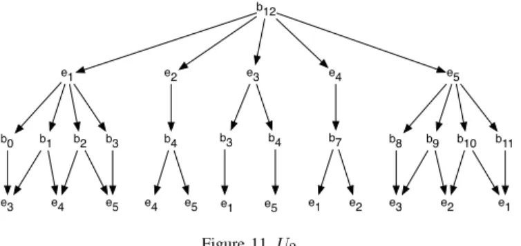
Let us consider the following Unfolding of Figure 11. The
e1 e2 e3 b12 b0 e4 e5 b2 b1 b3 e3 e4 e5 b4 e4 e5 b3 b4 e1 e5 b7 e1 e2 b8 b9 b10 b11 e3 e2 e1 Figure 11. U2.
table has been computed and the set of binaries relations between events leads to the following algebraic expression U2:
U2 = (⊕ b12 (b12≺ (e1⊥ e2 ⊥ e3⊥ e4⊥ e5)) (e1≺ (⊕ b0 b1b2 b3))(e2≺ b4)(e3≺ (⊕b5 b6)) (e5≺ (⊕b8 b9 b10b11))((⊕ b0 b1) ≺ e3) ((⊕ b1 b2) ≺ e4) (e4≺ b7) ((⊕ b2 b3) ≺ e5) (b4 ≺ (⊥ e4e5))(b5≺ e1) (b6≺ e5) (b7 ≺ (⊥ e1e2)) ((⊕ b8 b9) ≺ e3) ((⊕ b9 b10) ≺ e2) ((⊕ b10b11) ≺ e1)) (14)
Let us note P the aggregation of the five first lines of the previous Equation (14) becomes:
U2 = (⊕ b12 (b12≺ (⊥ e1 e2 e3 e4 e5)) P (15)
Rules M P 1, M P2 and theorem 1 reduce (15) in:
U2 = (⊥ (⊕ e1 P ) (⊕ e2 P ) (⊕ e3 P ) (⊕ e4 P ) (⊕ e5 P ) ) Distributivity of perp: U2 = (⊕ (⊥ (⊕ e1 b0 b1 b2 b3)(⊕ e2 b4)(⊕ e3 b5 b6) (⊕ e4 b7)(⊕ e5 b8 b9 b10b11)) ((⊕ b0 b1) ≺ e3) ((⊕ b1 b2) ≺ e4)((⊕ b2 b3) ≺ e5) (b4≺ (⊥ e4 e5)) (b5≺ e1) (b6≺ e5)(b7≺ (⊥ e1 e2)) ((⊕ b8 b9) ≺ e3) ((⊕ b9 b10) ≺ e2) ((⊕ b10 b11) ≺ e1)) Distributivity of ⊥ and M P1: U2 = (⊥ (⊕ e1 e3 e5 b1 b2)(⊕ e1 e4b0 b3)(⊕ e2 e4) (⊕ e2 e5) (⊕ e3 e1)(⊕ e3 e5)(⊕ e4 e1) (⊕ e4 e2)(⊕ e5 e1 e3 b9 b10) (⊕ e5 e2 b8 b11))
Theorem 2 : absorption of (⊕ e3 e1) and (⊕ e3 e5) in
(⊕ e1 e3 e5 b1 b2), idempotency of ⊥:
U2 = (⊥ (⊕ e1 e3 e5 b1 b2)(⊕ e1 e4 b0 b3)(⊕ e2e4)
(⊕ e2 e5) (⊕ e4 e1)(⊕ e5 e1 e3 b9 b10)
(⊕ e5 e2 b8 b11))
Rules of simplification S1and S2 and theorem 2:
U2= (⊥ (⊕ e1 e3 e5)(⊕ e1 e4)(⊕ e2 e4)(⊕ e2 e5))
The two unfoldings of examples 1 and 2 have the same canonic form, they are conflict-equivalent: U1≈conf U2
1) Reasoning about processes: Let us consider all the process p of U2: (⊕ e1 e3 e5), (⊕ e1 e4), ...
• ∀p ∈ U2 whenever e3 is present, e1 is present. • ∀p ∈ U2, ¬e3⊥ (e1⊕ e3⊕ e5)
This is the algebraic definition of ≺. Finally, from this chain of conflicts, the following causality can be deduced:
e3≺ (e1⊕ e5) (16)
• A similar reasoning can be made:
∀p ∈ U2, ¬(e1⊕ e5) ⊥ (e1⊕ e3⊕ e5)
This is the algebraic definition of:
(e1⊕ e5) ≺ e3 (17)
Equations (16) and (17) express that there is a strong link between e3 and the process (e1⊕ e5) but ≺ is no well
suited to encompass this relation. These two processes are like “intricated”.
• In the same manner:
¬e2⊥ (e2⊕ e4) ⊥ (e2⊕ e5)
≡dist¬e2⊥ (e2⊕ (e4⊥ e5))
≡def e2≺ (e4 ⊥ e5) (18)
e2 leads to a conflict
¬e1 ⊥ ((⊕e1e3e5) ⊥ (e1⊕ e4)
≡dist¬e1⊥ (e1⊕ ((e3⊕ e5) ⊥ e4))
≡def e1 ≺ ((e3 ⊕ e5) ⊥ e4) (19)
Equations (18) and (19) show that e1 and e2 transform the
chain of conflict in a unique conflict. New relations between events or processes can be introduced:
• Alliance relation: e1, e3 and e5 are in “an alliance
relation”. Every event of this set is enforced by the occurrence of the other events: e1⊕e3enforces e5, e1⊕e5
enforces e3 and e3⊕ e5 enforces e1.
• Intrication: the occurrence of e3 forces e1 ⊕ e5 and
reciprocally e1⊕ e5 forces e3. • Resolving conflicts (liberation):
– e1 resolves 3 conflicts on 4 (as e2, e4 and e5)
Semantically, e3can be identified as an important event in the
chain. Moreover, (⊕e1 e3 e5) is a process aggregated with
“associated events”. This chain of conflict can be seen as two causalities in conflicts:(e1≺ (e4⊥ (e3⊕ e5))) ⊥ (e2≺ (e4⊥
e5))
C. Example 3 (Cash dispenser)
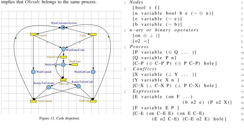
Let us consider a cash dispenser illustrated in Figure 12. The user has three tries (3 tokens are generated in place WaitEnterCode) to enter a valid code (OKcode), then he can get Cash or can Consult its account. In this example, a reset arc from OKCode allow to clear the tokens that have not be consumed (for example when the user has entered a valid code at its first or second try) and two reset arcs have been added from getConsult and getCash to clear ReadyT oConsult or ReadyT oGetCash.
It could be useful to prove that if the events GetCash implies that Okcode belongs to the same process.
3 3 1 WaitCustomerAction AnalyzeCode WaitEnterCode ReadyToGetCash WaitConsult WaitGetCash ReadyToConsult Consult GetConsult Cash EnterCode GetCash OkCode BadCode
Figure 12. Cash dispenser.
The unfolding of cash dispenser is given in Figure 13. A combinatory inflation of the net is caused by to the reset arcs and by the transitions, Consult and Cash, which produces 3 tokens each.
The reset arcs introduces for each events e9, e10, e11, e18,
e19, and e20(events relative the transition OKcode) two arcs,
which consumes adding conditions. The translation of reset arcs have been defined manually and is not yet implemented in reduction rules. The computing of the canonical form of the processes is following expression:
U 3 = (⊥ (⊕ Consult EnterCode OKcode GetConsult) (⊕ Consult EnterCode BadCode OKcode GetConsult)
(⊕ Consult EnterCode BadCode BadCode OKcode GetConsult) (⊕ Consult EnterCode BadCode BadCode BadCode)
(⊕ Cash EnterCode OKcode Getcash)
(⊕ Cash EnterCode BadCode OKcode Getcash)
(⊕ Cash EnterCode BadCode BadCode OKcode Getcash) (⊕ Cash EnterCode BadCode BadCode BadCode)
This expression formally proves that if GetCash is in a process then OkCode belongs to the same process.
VII. IMPLEMENTATION ASPECTS
A program [19] has been developed. It takes Petri Nets as inputs Romeo [20] unfolds and computes the canonical form. This program has been written in Lisp. The algebraic definitions and the reduction rules has been described with redex, a formal package introduced in [11].
A. Syntax of the language
The redex package allows to implement the syntactic rules of the language with an abstract and conceive way:
1 ; Nodes 2 [ b o o l t f ] 3 [ n v a r i a b l e b o o l b e ( ¬ ⊕ n ) ] 4 [ e v a r i a b l e ( ¬ e ) ] 5 [ b v a r i a b l e ( ¬ b ) ] 6 ; n−ary o r b i n a r y o p e r a t o r s 7 [ on ⊕ ⊥ o ] 8 [ o2 ≺ ] 9 ; P r o c e s s 10 [ P v a r i a b l e ( ⊕ Q . . . ) ] 11 [Q v a r i a b l e P n ] 12 [C−P ( ⊕ C−P P ) ( ⊕ P C−P) h o l e ] 13 ; C o n f l i c t s 14 [X v a r i a b l e ( ⊥ Y . . . ) ] 15 [Y v a r i a b l e X n ] 16 [C−X ( ⊥ C−X P ) ( ⊥ P C−X) h o l e ] 17 ; E x p r e s s i o n 18 [ E v a r i a b l e ( on F . . . ) 19 ( b o2 e ) ( P o2 X ) ] 20 [ F v a r i a b l e E P ] 21
[C−E ( on C−E E ) ( on E C−E)
22
( E o2 C−E) (C−E o2 E ) h o l e ] - The lines 2 to 5 define the basics nodes, which are
boolean, b conditions and e the events. The term variablein lines 3 to 5 allows to use in the language every symbols denoted as ni, bior ei. These symbols
are the terminal symbols of the alphabet.
- The lines 7 and 8 group the n-ary and the binary operators.
- Lines 10 to 12 define the process. A process P is constitued with ⊕ operator on Q, where Q is defined as a node n or a process P . Every non terminal symbol Pi is a process.
- Lines 14 to 16 define conflicts in a similar way. - Finally, lines 18 to 22 define expressions that are
built from conflicts, process and causality.
- For every term: Process, Conflicts and Expression, contexts are defined. The contexts capture prefixes
1
B 1 (WaitCustomerAction)
B 2 (WaitEnterCode)
B 3 (WaitEnterCode)
B 4 (WaitEnterCode) B 5 (WaitConsult) B 9 (WaitGetCash) B 6 (WaitEnterCode) B 7 (WaitEnterCode) B 8 (WaitEnterCode)
B 10 (AnalyzeCode) B 11 (AnalyzeCode) B 12 (AnalyzeCode) B 13 (AnalyzeCode) B 14 (AnalyzeCode) B 15 (AnalyzeCode)
B 16 (ReadyToGetCash) B 17 (ReadyToConsult) B 18 (ReadyToGetCash) B 19 (ReadyToConsult) B 20 (ReadyToGetCash) B 21 (ReadyToConsult) B 22 (ReadyToGetCash) B 23 (ReadyToConsult) B 24 (ReadyToGetCash) B 25 (ReadyToConsult) B 26 (ReadyToGetCash B 27 (ReadyToConsult) (WaitCustomerAction) B 29 (WaitCustomerAction) B 30 (WaitCustomerAction) B 31 (WaitCustomerAction) B 32 (WaitCustomerAction) B 33 (WaitCustomerAction) B 34 (WaitCustomerAction) B 35 (WaitCustomerAction) B 36 (WaitCustomerAction) B 37 (WaitCustomerAction) B 38 (WaitCustomerAction) B 39 (WaitCustomerActi E 1 (Consult) E 2 (Cash)
E 3 (EnterCode) E 4 (EnterCode) E 5 (EnterCode)
E 6 (EnterCode) E 7 (EnterCode) E 8 (EnterCode)
E 9 (OKcode) E 10 (OKcode) E 11 (OKcode) E 12 (OKcode) E 13 (OKcode) E 14 (OKcode)
E 15 (BadCode) E 16 (BadCode) E 17 (BadCode) E 18 (BadCode) E 19 (BadCode) E 20 (BadCode)
E 21 (GetConsult) E 22 (GetConsult) T 23 (GetConsult) E 24 (Getcash) E 25 (Getcash) E 26 (Getcash) E 27 (GetConsult) E 28 (GetConsult) E 29 (GetConsult) E 30 (Getcash) E 31 (Getcash) E 32 (Getcash)
Figure 13. Unfolding of Cash dispenser.
and suffixes of an expression and put them into a hole.
B. Reductions rules
Definitions have been implemented as reduction rules: (−−> ( i n − h o l e C−P ( ⊕ Q 1 . . . f Q 2 . . . ) ) ( i n − h o l e C−P f ) ”A⊕” ) (−−> ( i n − h o l e C−E ( ⊕ Q 1 . . . e 1 Q 2 . . . ( ¬ e 1 ) Q 4 . . . ) ) ( i n − h o l e C−E f ) ”F⊕” )
The particularities of this syntax are:
• Qi... is equivalent to the regular expression Q∗i, which
represents an ordered list of symbol Qi, which is
even-tually empty, finite or infinite.
• The contexts C-P or C-E allows to capture every sub-expression with every prefix and suffixe.
The first rule, labelled A⊕, illustrates that f is an absorbing
element. In this rule, C-P captures the context of a Process P and put into a hole. This reduction rule expresses that every sub-expression of the type (⊕Q1...f Q2...), which can
be reduced to the node f . This rule is named and thus, its use can be traced in a future proof.
The second rule F⊕ states the property defined in Section
IV-B4 : e1⊕¬e1≡ #f . This reduction rules defines that every
expression (for every context C-E) containing e1 and ¬e1 in
an ⊕ operator can be reduced to f .
C. Theorems
This section describes the implementation and the coding of theorems.
1) Theoreme 4: Theorem 4 has been stated from definition 6, which corresponds to the following statements:
( d e f i n e ( U1n n l ) ( i f (>= (− ( maxi l ) n ) 2 ) ( c o n s ( l i s t − r e f l ( + n 2 ) ) ( Rn ( + n 2 ) l ) ) empty ) ) ( d e f i n e ( V2n n l ) ( i f (>= (− ( maxi l ) n ) 3 ) ( c o n s ( l i s t − r e f l ( + n 3 ) ) ( Rn ( + n 3 ) l ) ) empty ) )
Finally, the implementation is coded like the union of the previous definitions:
( d e f i n e ( Rn n l )
( i f (>= (− ( maxi l ) n ) 1 )
( Union ( U1n n l ) ( U2n n l ) ) empty ) )
Note that the implementation of the definitions and the theorems are closed to their formal expression.
2) Theoreme 3: E ⊥ (E ⊕ F ) ≡ (E ⊕ F ) has been
implemented has a reduction rule: (−−> ( i n − h o l e C−E ( ⊥ E 1 . . . E E 2 . . . ( ⊕ E E 3 . . . ) E 4 . . . ) ) ( i n − h o l e C−E ( ⊥ E 1 . . . E 2 . . . ( ⊕ E E 3 . . . ) E 4 . . . ) ) ” T3 ” )
This code means that if E is in a “⊥ expression:” (⊥ E1... EE2...), then if a sub expression in ⊕ contains E, then
E can be suppressed of the “⊥ expression” for any context.
VIII. CONCLUSION AND FUTURE WORK
This work is a first attempt to present an axiomatic frame-work to the analyze of the processes issued of an unfolding. From a set of axioms, distributivities, and derivation rules, theorems have been established and a reduction process can lead to a canonic form. The unfolding process, definitions, theorems, and reduction rules have been coded in LISP[21] with a package named PLT/Redex[11][22]. This canonic form assets an equivalence conflicts (≡conf) between unfoldings
and then Petri nets.
Several perspectives are into progress. First, new theorems have to be established allowing to speed up the procedure of canonic reduction and to extend extraction of knowledge on relationship between events. Different kinds of relation-ship between events can be defined and formalized: Alliance relation, Intrication, etc. Moreover, as already outlined in the examples, algebraic reasoning can raise semantic informations about events from the canonic form. Another perspective is to extend the approach to Petri nets with inhibitor or drain arcs.
REFERENCES
[1] d. Delfieu, M. Comlan, and M. Sogbohossou, “Algebraic analysis of branching processes,” in Sixth International Conference on Advances in System Testing and Validation Lifecycle, 2014, pp. 21–27, best paper award.
[2] J. Esparza and K. Heljanko, “Unfoldings - a partial-order approach to model checking,” EATCS Monographs in Theoretical Computer Science, 2008.
[3] Engelfriet and Joost, “Branching processes of petri nets,” Acta Infor-matica, vol. 28, no. 6, pp. 575–591, 1991.
[4] J. Esparza, S. R¨omer, and W. Vogler, An Improvement of McMillan’s Unfolding Algorithm. Mit Press, 1996.
[5] McMillan and Kenneth, “Using unfoldings to avoid the state explosion problem in the verification of asynchronous circuits,” in Computer Aided Verification. Springer, 1993, pp. 164–177.
[6] C. A. R. Hoare, Communicating sequential processes. Prentice-hall Englewood Cliffs, 1985, vol. 178.
[7] R. Milner, Communication and concurrency. Prentice-hall Englewood Cliffs, 1989.
[8] C. A. Petri, “Communication with automata,” PhD thesis, Institut fuer Instrumentelle Mathematik, 1962.
[9] R. Glabbeek and F. Vaandrager, “Petri net models for algebraic theo-ries of concurrency,” in PARLE Parallel Architectures and Languages Europe, ser. Lecture Notes in Computer Science, J. Bakker, A. Nijman, and P. Treleaven, Eds. Springer Berlin Heidelberg, 1987, vol. 259, pp. 224–242.
[10] E. Best, R. Devillers, and M. Koutny, “The box algebra=petri nets+process expressions,” Information and Computation, vol. 178, no. 1, pp. 44 – 100, 2002.
[11] M. Felleisen, R. Findler, and M. Flatt, Semantics Engineering With PLT Redex. Mit Press, 2009.
[12] M. Nielsen, G. Plotkin, and G. Winskel, “Petri nets, event structures and domains,” in T. Theor. Comp. Sci., vol. 13(1), 1981, pp. 89–118. [13] J. Baeten, J. Bergstra, and J. Klop, “An operational semantics for process
algebra,” in CWI Report CSR8522, 1985.
[14] G. Boudol and I. Castellani, “On the semantics of concurrency: partial orders and transitions systems,” in Rapports de Recherche No 550, INRIA, Centre Sophia Antipolis, 1986.
[15] V. Glaabeek and F. Vaandrager, “Petri nets for algebraic theories of concurrency,” in CWI Report SC-R87, 1987.
[16] C. Dufourd, P. Janˇcar, and Ph. Schnoebelen, in Proceedings of the 26th ICALP’99, ser. Lecture Notes in Computer Science, J. Wiedermann, P. van Emde Boas, and M. Nielsen, Eds., vol. 1644. Prague, Czech Republic: Springer, Jul. 1999, pp. 301–310.
[17] T. Chatain and C. Jard, “Complete finite prefixes of symbolic unfoldings of safe time petri nets,” in Petri Nets and Other Models of Concurrency - ICATPN 2006, ser. Lecture Notes in Computer Science, S. Donatelli and P. Thiagarajan, Eds. Springer Berlin Heidelberg, 2006, vol. 4024, pp. 125–145. [Online]. Available: http://dx.doi.org/10.1007/11767589 [18] J.-Y. Girard, “Linear logic,” Theoretical computer science, vol. 50, no. 1,
pp. 1–101, 1987.
[19] D. Delfieu and M. Comlan, “Penelope,” http://penelope.rts-software.org/svn, Oct. 2013, tools for editing, unfolding and and to obtain canonical form for Petri Nets.
[20] G. Gardey, D. Lime, M. Magnin et al., “Romeo: A tool for analyzing time petri nets,” in Computer Aided Verification. Springer Berlin Heidelberg, 2005, pp. 418–423.
[21] G. L. Steele, Common LISP: the language. Digital press, 1990. [22] D. Delfieu and S. Mdssu, “An algebra for branching processes,” in
Control, Decision and Information Technologies (CoDIT), 2013 Inter-national Conference on, May 2013, pp. 625–634.