Algorithms for estimation and control of quadrirotors in physical interaction with their environment

HAL Id: tel-02895102

https://tel.archives-ouvertes.fr/tel-02895102

HAL is a multi-disciplinary open access archive for the deposit and dissemination of sci-entific research documents, whether they are pub-lished or not. The documents may come from teaching and research institutions in France or

L’archive ouverte pluridisciplinaire HAL, est destinée au dépôt et à la diffusion de documents scientifiques de niveau recherche, publiés ou non, émanant des établissements d’enseignement et de recherche français ou étrangers, des laboratoires

physical interaction with their environment

Quentin Delamare

To cite this version:

Quentin Delamare. Algorithms for estimation and control of quadrirotors in physical interaction with their environment. Robotics [cs.RO]. Université Rennes 1, 2019. English. �NNT : 2019REN1S099�. �tel-02895102�

T

HÈSE DE DOCTORAT DE

L’UNIVERSITÉ DE RENNES 1

COMUEUNIVERSITÉ BRETAGNE LOIRE

ÉCOLEDOCTORALEN°601

Mathématiques et Sciences et Technologies de l’Information et de la Communication

Spécialité : Automatique, Productique et Robotique Par

Quentin DELAMARE

Algorithmes

d’estimation

et

de

commande

pour

des

quadrirotors en interaction physique avec l’environnement

Thèse présentée et soutenue à Rennes, le 9/12/19 Unité de recherche : IRISA

Rapporteurs avant soutenance :

Nicolas Marchand Directeur de Recherche au GIPSA-lab, Université Grenoble-Alpes Pascal Morin Professeur à l’ISIR, Université Pierre et Marie Curie

Composition du Jury :

Président : Isabelle Fantoni Directrice de Recherche CNRS, LS2N Nantes Examinateurs : Isabelle Fantoni Directrice de Recherche CNRS, LS2N Nantes

Nicolas Marchand Directeur de Recherche au GIPSA-lab, Université Grenoble-Alpes Fabio Morbidi Maître de Conférences au MIS, Université de Picardie Jules Verne Pascal Morin Professeur à l’ISIR, Université Pierre et Marie Curie

Dir. de thèse : Paolo Robuffo Giordano Directeur de Recherche CNRS, IRISA/Inria Rennes Co-dir. de thèse : Antonio Franchi Chargé de Recherche CNRS, LAAS, Toulouse

Résumé de la thèse

Le domaine de la robotique aérienne est en plein essor grâce aux avancées tech-nologiques des dernières décennies. Le problème de la commande de ces systèmes volants, comme les quadrirotors par exemple, aura constitué un vrai défi du fait de leur sous-actionnement en général, et des phénomènes aérodynamiques complexes impliqués. Il faut noter que les techniques de commande développées sont principale-ment axées sur la captation de données et la cartographie en environneprincipale-ment ouvert. Au cours des dernières années cependant, le champ de la robotique aérienne pour l’interaction physique s’est beaucoup développé. Ce type de scénario fait intervenir un robot aérien devant appliquer un effort maîtrisé sur un objet ou sur l’environnement, alors qu’il vole. Des avancées significatives ont été réalisées, au travers notamment de projets européens centrés sur cette thématique, comme [2, 3, 8, 4].

Dans ces deux grandes familles d’approches, qui s’intéressent donc aux dépla-cements libres sans contact vs. avec interaction physique, l’environnement est gé-néralement traité comme une contrainte indésirée limitant les mouvements du robot. En d’autres termes, les tâches de déplacements libres/rapides et celles d’interactions physiques sécuritaires sont perçues comme antagonistes avec la présence d’éléments indésirés dans l’environnement. Une conséquence immédiate de ceci est que les mou-vements réalisés avec contact sont peu dynamiques. En s’inspirant de l’utilisation des contacts faite en robotique humanoïde, nous proposons dans cette thèse d’exploi-ter le contact physique avec l’environnement dans le but de réaliser de la locomo-tion aérienne. Autrement dit, nous proposons de considérer l’environnement comme une source de contacts exploitables à des fins de locomotion, plutôt que comme une contrainte à éviter. Avec cette approche, nous souhaitons exploiter pleinement la dy-namique des robots aériens en interaction physique.

Dans la première partie de cette thèse, nous détaillons les travaux réalisés relatifs à ce concept de locomotion aérienne. Cette idée est étudiée et démontrée au travers de simulations et expérimentations d’une nouvelle plate-forme robotique aérienne consis-tant en un quadrirotor équipé d’un bras robotique à un degré de liberté. Le premier chapitre détaille la dynamique particulière de ce système, qui comporte trois modes de fonctionnement différents. Les deux plus évidents correspondent aux dynamiques

collision est proposé pour comprendre et intégrer au mieux ce phénomène dans les développements consécutifs. Deux stratégies de commande sont également données afin de permettre à ce robot de suivre une trajectoire en temps-réel.

Dans le deuxième chapitre nous expliquons la démarche entreprise afin de mettre en place un algorithme d’optimisation de trajectoires adapté à ce système. Un cas élémentaire de locomotion est choisi, dans lequel le système doit exécuter une ma-nœuvre partant d’une configuration initiale en contact avec l’environnement (le bras "s’accroche" à un premier point de pivot), et terminant dans une configuration avec un autre point d’attache plus loin, en passant par une phase intermédiaire de vol libre. La structure du planificateur de trajectoires développé lui permet d’intégrer le compor-tement dynamique complet du robot, y compris une possible collision comme évoqué précédemment, ce qui lui donne la possibilité de tirer au mieux parti de ses particula-rités. Une fonction de coût spécifique est également développée afin de garantir une précision maximale du robot dans la phase la plus critique. Des trajectoires sont en-suite générées pour différentes conditions, à savoir pour différentes limites d’actionne-ment et quelques variations de la fonction de coût minimisée. Les trajectoires obtenues sont ensuite analysées au regard de la tâche de locomotion considérée.

Pour terminer, le chapitre 3 expose les détails de conception et de réalisation d’un prototype en vue de tester les simulations précédentes. Un système d’attache magné-tique est développé puis réalisé et testé, ce qui permet au robot de s’attacher au point de pivot dans des conditions propices à la locomotion. La phase de conception de ce sous-système est détaillée, notamment la modélisation de celui-ci qui a été réalisée en vue de simuler son comportement magnéto-mécanique et d’optimiser sa performance au vu des conditions. Le comportement thermique de ce sous-système est également modélisé afin d’assurer un fonctionnement nominal non destructif. Des éléments de conception mécanique sont également donnés.

Dans la seconde partie, nous nous intéressons au problème de la précision réali-sable par un robot en suivi de trajectoire lorsque le modèle est incertain, et plus préci-sément lorsque les paramètres du modèle sont entachés d’erreur. Une généralisation de la fonction de coût spécifique introduite auparavant (au chapitre 2) est proposée, améliorant le concept tout en le rendant applicable à une large gamme de robots. En

effet, nous avons étudié le problème de la génération de trajectoires dont la sensibilité aux paramètres du modèle de robot considéré est minimale, dans le cas général. Ce type de trajectoires est généralisé à n’importe quel robot présentant une dynamique avec des incertitudes sur les paramètres, et se révèle particulièrement approprié dans le cas du quadrirotor étudié dans cette thèse, du fait de l’incertitude importante concer-nant ses paramètres inertiels et d’actionnement. Pour traiter ce problème, nous propo-sons donc la nouvelle notion de "sensibilité de l’état aux paramètres en boucle fermée" et nous montrons comment cette quantité peut être utilisée dans un contexte d’optimi-sation de trajectoires afin de générer des trajectoires dont la sensibilité aux paramètres est minimale, garantissant ainsi une forte robustesse.

Le chapitre 4 propose une première approche de ce concept pour produire des trajectoires dites à “sensibilité minimale”, avec des analyses statistiques afin de tester l’efficacité de la méthode. Plusieurs cas sont considérés, faisant intervenir un robot mobile différentiel (unicycle) et un quadrirotor avec des lois de commande comprenant ou non un intégrateur, et avec une minimisation soit de la sensibilité de l’état final, soit de la sensibilité de l’état sur l’ensemble de la trajectoire (avec un coût intégral). Il en ressort que la méthode semble bien fonctionner en simulation pour les cas considérés, à savoir que les trajectoires générées donnent lieu à une erreur de suivi moindre par comparaison avec des trajectoires non optimisées ayant les mêmes conditions limites lorsque les paramètres du modèle sont mal calibrés.

Finalement, le chapitre 5 propose une généralisation de la méthode afin de produire une théorie plus générale, rigoureuse, et susceptible d’être appliquée plus largement à différents types de robots. Entre autres, la possibilité d’avoir une loi de commande imparfaite, c’est-à-dire, ici, qui n’est pas capable d’annuler l’erreur de suivi en dépit de paramètres bien calibrés et d’absence de perturbations, est intégrée dans la méthode. D’autres métriques issues de la sensibilité sont également calculées. En particulier, une utilisation de la sensibilité des entrées par rapport aux paramètres est proposée pour pallier leur manque de prédictibilité observé dans certains cas. Plusieurs ana-lyses statistiques sont ainsi réalisées sur des simulations, avec des résultats validant là aussi les méthodes proposées en terme de réduction d’erreur. Enfin, une série d’ex-périmentations est menée sur un robot réel de type robot mobile différentiel (modèle Pioneer 3DX), validant également la méthode en améliorant les performances de suivi de trajectoire obtenues.

Les éléments développés dans cette thèse ont fait l’objet de trois publications scien-tifiques listées ici :

(a) Q. Delamare, P. Robuffo Giordano, and A. Franchi, “Toward aerial physical lo-comotion : The contact-fly-contact problem,” in IEEE Robotics and Automation Letters (RAL), vol. 3, no. 3, pp. 1514–1521, 2018, au sujet de la locomotion aérienne. Un algorithme de génération de trajectoires adapté à cette tâche par-ticulière y est présenté et testé en simulation.

(b) P. Robuffo Giordano, Q. Delamare, and A. Franchi, “Trajectory generation for mi-nimum closed-loop state sensitivity,” in 2018 IEEE International Conference on Robotics and Automation (ICRA), 2018, concernant la génération de trajectoires minimisant la sensibilité de l’état aux paramètres. Une analyse statistique y est présentée qui valide l’utilité et l’efficacité de l’algorithme présenté.

(c) N. Staub, M. Mohammadi, D. Bicego, Q. Delamare, H. Yang, D. Prattichizzo, P. Robuffo Giordano, D. Lee, A. Franchi, “The Tele-MAGMaS : an Aerial-Ground Co-manipulator System,” in 2018 IEEE Robotics and Automation Magazine (RAM), vol. 25, no. 4, pp 66–75, 2018, qui présente un système de co-manipulation fai-sant intervenir un hexacoptère spécial et un manipulateur au sol en coopération pour mouvoir un objet.

Plusieurs vidéos ont été réalisées afin d’illustrer les résultats principaux associés à ces travaux, concernant la locomotion aérienne1_{, la génération de trajectoires à}

sensi-bilité minimale2_{, et le système Tele-MAGMaS présenté à la Hannover Fair à l’occasion}

des KUKA Innovation Awards3 4_.

1. video at https ://proxy.ens-rennes.fr/owncloud/index.php/s/Nrx5Rmm9S93TsmF 2. video at https ://proxy.ens-rennes.fr/owncloud/index.php/s/nxFbMCRzD7wCzQp 3. video at https ://proxy.ens-rennes.fr/owncloud/index.php/s/KZgB2TCAYfoJ6wW 4. video at https ://proxy.ens-rennes.fr/owncloud/index.php/s/6ZBXsf9peCaHX52

R

EMERCIEMENTS

Je tiens à remercier pour commencer mes directeurs de thèse, Paolo et Antonio, qui ont su faire preuve au cours de ces trois années d’un enthousiasme à toute épreuve et d’une ingéniosité riche et insolite, ce qu’il me fallait. Je remercie également les mem-bres de l’équipe Rainbow pour la bonne ambiance qui y règne. Un grand merci aux in-génieurs pour leur aide précieuse, Fabien, Pol, Thomas, ainsi qu’à Marie pour m’avoir permis d’accéder aux ateliers de l’INSA. Merci également à Tristan et Pascal pour les chouettes moments partagés durant leurs stages. Merci aussi aux collègues de l’ENS, qui m’ont accompagnés et soutenu dans cette aventure tant sur le plan scientifique que sur le plan de l’enseignement. Merci à tous ceux avec qui j’ai partagé de super sessions musicales.

Je remercie également mes proches pour leur soutien et leur patience (il en fallait). Merci à ma famille et Evelyne d’avoir été là plus que je n’ai été là pour eux. Je vous dois beaucoup. Merci aussi aux trois Fontaine de m’avoir abreuvé de moments de bonheur partagés, de randos (promis on l’aura ce vieux caillou), et autres repas à gogo. Merci à Simon pour ces 10 ans de bidouilles en tout genre (ce n’est que le début) et pour ces moments passés tous les 4, et merci aux Mektro12 pour le chemin parcouru ensemble.

Enfin je remercie Anaïs qui, au-delà de son indéfectible soutien, est le beurre salé de mes galettes, et avec qui je suis fier de partager la valse de la vie.

T

ABLE OF

C

ONTENTS

Introduction 13

Context . . . 13

Overview of the state of the art . . . 14

Aerial robotics . . . 14

Trajectory generation . . . 16

Thesis contributions . . . 18

Thesis structure . . . 19

I

Part I

21

1.4 Validation of the Control Strategy . . . 33

1.5 Conclusion . . . 35

2 Trajectory planning for the MonkeyRotor 37 2.1 Introduction . . . 37

2.2 Planning algorithm . . . 37

2.2.1 Optimization procedure . . . 38

2.2.2 Cost function . . . 41

2.3.1 Trajectory planning . . . 43

2.3.2 Trajectory tracking . . . 47

2.4 Conclusion . . . 48

3 Conception of the MonkeyRotor prototype 53 3.1 Introduction . . . 53

3.2 Design of the hooking system . . . 53

3.2.1 General concept . . . 53

3.2.2 Choice of the solution . . . 55

3.2.3 Magnetic coil design . . . 56

3.2.4 Rotating joint design . . . 69

3.3 Implementation . . . 70

3.3.1 Hardware manufacturing . . . 70

3.3.2 Software structure . . . 72

3.4 Conclusion . . . 73

II

Part II

77

4.2 Open-loop state sensitivity . . . 81

4.2.1 Simple integrator case . . . 82

4.2.2 More complex dynamics . . . 84

4.2.3 Computation of the sensitivity in the general case . . . 86

4.3 Closed-loop sensitivity . . . 88

4.3.1 Motivation . . . 88

4.3.2 Derivation . . . 89

4.4 Application to robotic trajectory generation . . . 92

4.4.1 Unicycle dynamics and control . . . 92

4.4.2 Planar quadrotor dynamics and control . . . 94

4.4.3 Trajectory generation . . . 97

4.4.4 Gradient derivation . . . 100

4.4.5 Simulations . . . 103

TABLE OF CONTENTS

4.6 Conclusion . . . 111

5 Improvements and generalization of the sensitivity minimization frame-work 113 5.1 Introduction . . . 113

5.2 Generalization to arbitrary outputs . . . 114

5.2.1 Solving procedure in the general case . . . 123

5.2.2 Final error compensation case study . . . 127

5.3 Other sensitivity metrics . . . 128

5.4 Statistical analysis . . . 131

5.5 Experimental validation . . . 137

5.6 Conclusion and perspectives . . . 143

Conclusion 145

I

NTRODUCTION

It is nowadays common to see quadrotor UAVs both in the domain of public enter-tainment with a large range of commercial products, as well as in professional appli-cations such as remote inspection, cartography, agricultural spraying, or even filming. As well known, this flourishing of the field of aerial robotics has been made possi-ble thanks to the common progress of on-board computational capabilities, together with the miniaturization of the associated electronics and power cells. Indeed, the mass/energy ratio of modern lithium-based batteries coupled with the high efficiency of synchronous motors allow the conversion of enough mechanical power to keep a multirotor aircraft in hover flight, for a non negligible duration. Moreover, the associated control algorithms have been heavily developed together with the computing capacity of on-board electronics.

As a result, current multirotor robots are more than ever autonomous, and present a huge potential for future robotic applications with complex tasks in complex environ-ments. It is clear however that this kind of robotic platforms are challenging to control by nature, because of the complex aerodynamics of the rotating propellers (especially when close to a surface or in adverse wind conditions) and because of their freedom in the 3D environment. The possibilities are thus vast, but still a lot of challenges need be dealt with to make this kind of aerial robots able to handle complex real-world situ-ations. To this extent, the field of aerial robotics have been developed a lot during the past decade, with substantial improvements in the control and localization of multirotor robots.

Context

The development and control of multirotor UAVs can be considered a practically solved problem for a wide range of navigation applications, mainly with surveillance or sensing tasks. Indeed, small aircrafts such as quadrotors are well suited to navigation tasks in tight or complex environments, because of their interesting agility and low price. Their relatively low weight associated with their important actuation capabilities

(in terms of force and torques) allows highly dynamical motions, thus such robots can achieve maneuvers that are adapted to difficult environments, for example in rescue or exploration applications.

Simultaneously, a number of recent works have also studied the possibility of having a contact between such a multirotor aircraft and its environment in the past years, which extends the robot applications a lot. The three main motivations for such studies are the ability of multirotors to

1. grasp some objects in the environment and displace them,

2. apply a force or, more generally, a wrench to some part of the environment such as a switch on a wall, a door handle to turn or some mechanism to screw (as can be found in the DARPA challenge for instance),

3. perform a proper (smooth) landing with special properties, e.g., land against a wall or on a moving platform [25, 46].

However, in these applications of aerial physical interaction, the structure of the environment is always a source of constraints that must be avoided in order to pre-serve both the integrity of the robot and of the environment. This is even more true for complex environments such as in indoor applications or in cluttered urban or industrial places, where possible collisions are numerous. As a consequence, in this kind of ap-plications, the behavior of aerial robots is mostly bounded by the need to avoid or to master the contacts with the environment.

Overview of the state of the art

Aerial robotics

In this context, numerous works have been conducted to assess the problems of estimation and robust command of quadrotors. The specific dynamics of this kind of aerial robot have been studied and leveraged so that, with the proper framework, one can locate and control them in order to track desired trajectories, see e.g. [22, 36, 44, 37]. The problem of the servoing of these robots has also been studied with a lot of different approaches, e.g., [37, 14, 22, 15, 53], ranging from sliding mode to H-infinity or LQR. These works propose control algorithms that either focus on the robustness, or on the fastness of the control loop.

Introduction

Note that in the vast majority of these works, the sensing relies on an external localization structure such as indoor motion capture in order to retrieve the location of the aircraft. A number of studies propose methods to improve the sensing component by means of on-board sensors (mainly vision) and relevant associated algorithms [27, 45, 56, 1]. More recently, we have also seen methods that are able to treat cases where only low quality information is available for sensing [52].

As stated before, the main applications of these works deal with navigation and data acquisition, which places the focus on the flight of the quadrotor itself. However, recent research has begun to leverage their operational potential in order to make them physically interact with their environment. With this kind of approach, the quadrotors can be used as aerial manipulators able to interact. The corresponding research field is called Aerial PHysical Interaction (APhI). For instance, [70, 54, 55] have explored the possibility for a multirotor equipped with an on-board ‘manipulator‘ (active or passive) to achieve manipulation tasks. Interestingly, we have also seen a few new concepts in the past years that tend to push the boundaries of multirotor capabilities by means of original features, e.g., [71] which studied an original stabilizing fast perching, or [7] which proposed a multi-part aerial robot with variable configuration for grasping, but also [61] which propose a framework for aerial interaction that is based on a special hexarotor with tilted propellers, thus fully actuated.

In parallel, some works have been focused more on the high level interaction with an operator, e.g., [26, 60], proposing algorithms for conveying information between an operator and the actual contact at best. This area of research presents several challenges since translating the control methods from grounded robots with physical interaction to equivalent aerial situations is not straightforward. This field have also been supported through the past years by large international projects such as [2, 3, 8, 4], which have focused on complex scenarios that tend to be more realistic.

As a consequence, we see that the current state of the art allows one to achieve some aerial robotic task with interaction with the environment. However, in all these works the interaction remains either highly restrictive, or needs to be controlled to follow a mastered mechanical wrench. Therefore, in this thesis we propose to change this perspective by considering the environment as a source of possible contacts that can be leveraged for the sake of locomotion. Indeed, the aerial robot may be able to benefit from the way certain particular contacts affect its dynamics, and thus achieve complex movements that improve its maneuverability.

Figure 1 – Examples of modern applications of aerial robotics. On the left, a commercial product that is designed for waterproof rescue missions. On the middle, a foldable quadrotor able to adapt its shape from [23]. On the right, a cooperative framework sharing the task of moving an object between a grounded manipulator and an aerial robot, from [60].

Trajectory generation

The second topic we are interested in throughout this thesis is the generation of robotic trajectories, in particular for mobile robots. Indeed, the foreseen concept of aerial locomotion is closely related to the ability of our algorithms to plan trajectories that achieve the desired maneuvers. This kind of behavior also rely a lot on the ability of the robot to track precisely the planned trajectory via its controller.

Research has been conducted on these subjects over the years, that led to different kind of strategies for trajectory generation. One of the most used techniques for gener-ating feasible trajectories that minimize some cost consists in leveraging the flatness of the robot, whenever this property is available. This concept was introduced in [24] and exploited for trajectory generation in [50]. Basically, featuring this property for a dynam-ical system means that it is possible to express both its input and output as functions of a certain ‘flat output‘ (and possibly some of its derivatives). In practice, this allows to easily compute the state of the system given a certain trajectory of the flat output, by means of an algebraic relation and thus without needing to integrate the dynamics. This makes the trajectory generation much more efficient in theory. A known pitfall of this method, however, is that the expression for the input (as function of the flat out-put) is often highly non-linear and computationally heavy, and thus tend to cancel the benefit of the method in cases where the actuation is part of the optimized elements, e.g., in presence of actuation bounds. Moreover, this relation as well as the one for the state require an high accuracy in the model parameters and often include the position of some center of mass and inertia which are difficult parameters to measure.

Introduction

The most common other methods for generating trajectories are simple direct tran-scription, i.e., forward integration of the dynamics, but also direct collocation [9]. The method of the (orthogonal) collocation consists of using orthogonal polynomials to rep-resent at the same time the input and output of the dynamics at knot points. Contrary to the flatness method or direct transcription where the dynamics is intrinsically re-spected by construction, here the relation between the input and output of the robot is enforced as a constraint at each considered knot point (but not between them in general). The precision of this approximation remains however controlled and can be arbitrarily reduced by increasing the number of considered knot points.

A number of works have applied these methods to multirotor UAVs in the past years, e.g., [57, 58, 67, 28, 52], with great success in the obtained performances. In all these studies, the achieved planned trajectories make it possible to optimize an objective (performance of a parameter estimation, observability) and/or respect special con-straints (collision avoidance, actuation limits). However, we note that in these works the trajectory tracking remains decoupled from the planning stage. Hence, the achieved performance when tracking the planned trajectory is bound to the strict respect of the conditions that are envisioned for the planning. In particular, any discrepancy that was not modeled at the planning stage, i.e., disturbances, unmodeled phenomena or poorly calibrated model, needs to be compensated by the real-time control loop, which will inevitably affect the tracking performance in an unmastered and potentially high pro-portion in case of inaccurate modeling.

Another kind of approach is to handle this difficulty by means of strategies that rely on a human-in-the-loop, see e.g. [42, 43, 41]. With such methods, some part of the task realization is given to the responsibility of the operator, which allows good compromises between the flexibility of the human operator and the achievable precision and strength of the robot.

Finally, a more recent class of strategies try to integrate the behavior of the control-loop at the planning stage in order to build ‘control-aware‘ schemes that leverage at most the information of the models, like in [28, 6, 21]. In this last kind of works, the way that the controller will behave during execution of the trajectory is taken into account from the planning stage. This approach makes the complete stack planner–controller more tightly coupled by making the planner ‘aware‘ of the real-time control loop.

In this thesis we will propose a control-aware trajectory planning framework that is adapted to robots with uncertain parameters, such as aerial robots which feature

complex aerodynamics that are difficult to model and compensate precisely.

Thesis contributions

In this thesis we develop strategies for trajectory generation, with the purposes of improving aerial locomotion capabilities, and improving the tracking of trajectories for systems that feature poorly known parameters. In particular, we focus on the two main issues that are raised when considering aerial locomotion, which are

1. the generation and tracking of trajectories for an aerial robot with switching dy-namics,

2. the generation of trajectories that are robustly tracked in presence of model parameter uncertainties.

The study of these thematics led to a new trajectory planning algorithm for aerial locomotion, described in

1 Q. Delamare, P. Robuffo Giordano, and A. Franchi, “Toward aerial physical lo-comotion: The contact-fly-contact problem,” in IEEE Robotics and Automation Letters (RAL), vol. 3, no. 3, pp. 1514–1521, 2018.

A video demonstrating simulations of the resulting trajectories for aerial locomotion is available5_{. A prototype have also been realized in the course of the thesis, including}

a magnetic hooking system and the robotic platform of the MonkeyRotor, which will allow further explorations of the concept of aerial locomotion.

Then, we developed a novel trajectory optimization framework for mobile robots with uncertain models, based on sensitivity metrics, which led to the following contribution:

2 P. Robuffo Giordano, Q. Delamare, and A. Franchi, “Trajectory generation for minimum closed-loop state sensitivity,” in 2018 IEEE International Conference on Robotics and Automation (ICRA), 2018,

This work was synthesized in a video showing the improvement in the tracking per-formance when using a trajectory that is optimized w.r.t. the closed-loop state sensitiv-ity, for a unicycle and a quadrotor6_{. It also led to further developments and validations}

of this theory as described in the last chapter of thesis, including new metrics of interest based on the sensitivity.

5. video at https://proxy.ens-rennes.fr/owncloud/index.php/s/Nrx5Rmm9S93TsmF 6. video at https://proxy.ens-rennes.fr/owncloud/index.php/s/nxFbMCRzD7wCzQp

Introduction

Finally, in relation with these two fields, we also participated in the development of the Tele-MAGMaS project presented at the Kuka Innovation Awards 2017 (finalist), which led to the following paper:

3 N. Staub, M. Mohammadi, D. Bicego, Q. Delamare, H. Yang, D. Prattichizzo, P. Robuffo Giordano, D. Lee, A. Franchi, “The Tele-MAGMaS: an Aerial-Ground Co-manipulator System,” in 2018 IEEE Robotics and Automation Magazine (RAM), vol. 25, no. 4, pp 66–75, 2018.

A video of the realized simulation framework is available7_{, as well as a video of the}

Hannover Fair demonstration8_.

Thesis structure

This thesis is split in two main parts. The first one, Part I, is dedicated to the study of the MonkeyRotor, a robot concept whose goal is to evaluate the properties and benefits of aerial locomotion. The second part, Part II, contains the theoretical development and validations of a new trajectory generation framework that aims at improving the track-ing performances of robots — especially when subject to uncertainties in their model parameters.

Outline of Part I

In this part, we develop the contact-fly-contact problem which is a case-study of aerial locomotion. The MonkeyRotor is introduced as the aerial robot dedicated to the study of this problem.

Chapter 1 provides an analysis of the particular dynamics and control of the

Mon-keyRotor. The specificities of this robot and how they can be leveraged in the context of aerial locomotion are discussed.

Chapter 2 details the trajectory generation algorithm that was designed for this

sys-tem. We show the important features of the realized aerial locomotion, with an analysis of the resulting generated trajectories among different planning conditions.

Chapter 3 gives the details about the realization of a prototype of the MonkeyRotor.

A novel magnetic hooking system is designed and realized, that makes it possible for

7. video at https://proxy.ens-rennes.fr/owncloud/index.php/s/KZgB2TCAYfoJ6wW 8. video at https://proxy.ens-rennes.fr/owncloud/index.php/s/6ZBXsf9peCaHX52

the system to alternate between states with and without contact as wished.

Outline of Part II

This part is dedicated to the novel algorithm for the generation of ‘minimum sensi-tive‘ trajectories.

Chapter 4 proposes a method that allows to generate trajectories resulting in a

minimization of the tracking error that are due to erroneous calibration of the model parameters. A statistical analysis is conducted which validates the soundness of the concept, based on a Monte Carlo simulation campaign.

Chapter 5 provides a generalization of the theory to robots that have controllers with

arbitrary tracking performance (including lag or filtering behaviors). Other sensitivity metrics of interest are also proposed which improve the robustness of the overall task realization. The concept is validated through large scale statistical analysis and real experiment on a unicycle.

PART I

CHAPTER1

M

ONKEY

R

OTOR CONCEPT AND

ANALYSIS

1.1

Introduction

In this chapter we will describe the theoretical study of a new robotic concept. As stated in the main introduction, the starting point lies in the observation that in aerial robotics the environment is usually considered as an obstacle to be avoided, or more generally, as a constraint. Conversely, in this Thesis we focus on the possibility of ex-ploiting a contact between the aerial robot and the environment for the sake of enhanc-ing the navigation capabilities.

To do so, we isolate a particular case-study which consists in making a quadrotor equipped with an arm able to locomote under two pivot points. More precisely, the goal of such a robot is to navigate through its environment not only by means of its own ability to fly, but also with phases where a physical contact with the environment happens and is leveraged to the benefit of the overall maneuver. This aerial robot thus has a particular dynamics because of its ability to be in physical contact with its environment. Figure 1.1 illustrates a possible depiction of this system when realizing a maneuver that utilizes a contact with a pivot point.

1.2

Dynamical modeling

The MonkeyRotor consists of a quadrotor UAV equipped with an actuated 1-DOF arm meant to grasp a pivot point (e.g., a branch) in the environment with its end-effector. In this section we illustrate the dynamical model of the MonkeyRotor during the two phases, i.e., hooked and free-flight, by borrowing from the previous works [69, 65] which have considered similar scenarios. In particular, [69] has considered a quadrotor

Figure 1.1 – Illustration of the concept of the MonkeyRotor: a quadrotor equipped with an arm which leverages a pivot point in the environment in order to achieve aerial locomotion.

with actuated arm but only in free-flight, while [65] has considered the hooked case but with a passive arm. As already done in many previous works on similar subjects, see, e.g., [29, 64, 49, 69, 65], we restrict the analysis to the vertical plane.

1.2.1

Definitions

With reference to Fig. 1.2, let FW be an inertial world frame with axes {xW, zW}

and origin OW, and FBa body frame attached to the quadrotor with axes {xB, zB}: the

axis zB represents the body-frame thrust direction, and the origin OB is placed at the

quadrotor center of mass (CoM). The configuration of the quadrotor can be specified by the position of OB in FW, denoted as pB = [xB zB]T ∈ R2, and the orientation of FB

w.r.t. FW here parametrized by the angle θB from zW to zB.

1.2. Dynamical modeling LB p1 d1 L1 ut ur τ fl fr θB θ1 pE xW zW OW OB zB x_B

Figure 1.2 – Geometry of the MonkeyRotor, a flying robot with an actuated arm. quadrotor CoM pB, around which it can rotate by an angle θ1defined as the angle from

zB to the arm direction. The CoM of the arm, denoted as p1, is placed at a distance

d1 from OB. The configuration of the whole MonkeyRotor (quadrotor + arm) is then

denoted as q = [pT

B θT]T ∈ R4 where we let θ = [θB θ1]T.

The quadrotor is equipped with two propellers generating two thrust vectors flzB

and frzB: the forces produced by the propellers result in a total thrust vector utzB =

(fr + fl)zB and torque ur = L₂B(fr − fl), with LB being the distance between the two

propellers. The arm is also assumed actuated by a torque τ acting at OB. These three

inputs for the whole MonkeyRotor are then denoted as u = [ut ur τ ]T ∈ R3. For

conve-nience, we also define the alternative input vector uf = [fr fl τ ]⊤= Ku where

K=      1/2 1/LB 0 1/2 −1/LB 0 0 0 1      . (1.1)

Indeed, while the MonkeyRotor dynamics are more naturally expressed in terms of the input vector u, the physical actuation constraints, i.e., min and max joint torque and propeller thrusts, affect the input uf. This distinction will be important in the next

developments. We finally let mB, JB, m1, J1 be the mass and inertia of the quadrotor

We now describe the dynamical model of the MonkeyRotor in the two considered phases of hooked and free-flight.

1.2.2

Hooked phase

represent the position of the arm end-effector in FW and p∗E ∈ R2 the (fixed) position

of the hook in FW. Following [65], the hook constraint pE(q) = p∗E restricts the

Mon-keyRotor motion to a circle centered at p∗

E. In this constrained case the MonkeyRotor

configuration is fully determined by the configuration variables θ: by applying standard techniques (Euler-Lagrange procedure), one can then obtain the following (reduced) dynamical model governing the behavior of the states (θ, ˙θ)

Mh(θ)¨θ+ gh(θ) = Gh(θ)u (1.3) where M_h(θ) =   JB 0 0 J1 + mBL21+ m1(L1− d1)2  , (1.4) Gh(θ) =   0 1 −1 L1sin(θ1) 0 1  , (1.5)

and gh(θ) = [0 (mBL1+m1(L1−d1))g sin(θB+θ1)]⊤. Since the matrix Gh(θ) is always full

rank, the hooked MonkeyRotor is overactuated, with two controlled variables θ for the three control inputs of u. We note that in [65] the joint arm was considered passive, i.e.,

τ = 0 thus resulting in a fully-actuated system with a singularity for θ1 = 0 as opposed

to the case under consideration which is singularity-free. Sect. 1.3.1 will elaborate more about the possible use of the MonkeyRotor overactuation.

The behavior of the remaining MonkeyRotor states (pB, ˙pB) can then be

alge-braically expressed as a function of θ and ˙θ by exploiting the hook constraint pE(q) =

p∗ E as pB = p∗E− L1   − sin(θ1 + θB) cos(θ1+ θB)   (1.6)

1.2. Dynamical modeling and ˙pB = L1( ˙θ1+ ˙θB)   cos(θ1 + θB) sin(θ1+ θB)  . (1.7)

1.2.3

Free-flying phase

The free-flying dynamical model of the MonkeyRotor is a particular case of the system presented in [69]. In particular one has

Mf(q)¨q+ cf(q, ˙q) + gf(q) = Gfu, (1.8)

where the expression of the various terms are given in [69].

We note that, as opposed to the hooked scenario, the MonkeyRotor is underactu-ated during free-flight (three inputs u for four configuration variables q). However, as discussed in [69], it is possible to find a flat output or linearizing output [24] which al-lows for full dynamic linearization of the system dynamics. More details about this point are given in Sect. 1.3.2.

1.2.4

Impact Model

One particularity of the concept of aerial locomotion is that the contact between the end-effector of the robot and the pivot point is possibly accompanied by a voluntary shock, which means that the hooking event itself may not be smooth for the sake of the global maneuver. Indeed, let th be the time at which the MonkeyRotor switches from

a free-flight phase to a hooked phase because the end-effector has reached the pivot location p∗

E and performed a successful hook. If ˙pE(t−h) 6= 0, i.e., the end-effector

ve-locity is non-zero just before hooking, a sudden impact will occur affecting the evolution of the MonkeyRotor state (q, ˙q).

Therefore, the goal of this section is to propose a simple impact model based on impulse theory, see, e.g., [47] able to capture the instantaneous change from ˙q(t−

h)

to ˙q(t+

h) because of a possible collision between the end-effector and the hook. As

customary, we assume continuity of q, i.e., q(t−

h) = q(t+h), in presence of an

instan-taneous impact [47]. The availability of this impact model will then allow us to have a complete model of the MonkeyRotor full dynamics that integrates the effects of a pos-sible collision. In a trajectory planning context, as it will be done later in this Thesis,

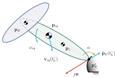
this allows the planner to be ‘aware’ of the possible collision, and thus generate more realistic motion plans that can also take advantage of this . For example, as far as the feasible trajectory space is large enough, the collision between end-effector and pivot can be controlled by the trajectory planner for quickly reducing the system kinetic en-ergy. Conversely, the magnitude of the impact can also be reduced in the same way if necessary. jn p1 p_eq pB p∗ E ˙pE(t−h) α ωeq v_eq(t− h)

Figure 1.3 – Notations for the collision model. The large and ‘instantaneous’ reaction force at E is synthesized in the impulse vector jn.

Recalling that ˙q = [ ˙pT B ˙θ

T

]T, we first consider the effects on the two angular veloc-ities ˙θ = [ ˙θB ˙θ1]T. First of all, we remark that the choice of placing the joint base at

the quadrotor CoM — a property also known as protocentricity [66] — implies that the rotational dynamics of the quadrotor base is completely decoupled from the dynamics of the collision. Indeed, the efforts that are transmitted through the arm joint are only linear forces (no torque), which do not generate any torque on the quadrotor base as they are directly applied to its CoM without offset. Therefore one has ˙θB(t+h) = ˙θB(t−h),

i.e., the rotational velocity of the quadrotor base is not affected by the impact. Concern-ing the angular velocity of the arm after the impact, we compute it by assimilatConcern-ing the MonkeyRotor to an equivalent body with the following properties for the sake of impact modeling:

1.2. Dynamical modeling

— CoM peq=

mBpB+ m1p1

meq

— inertia Jeq = J1+ m1kp1− peqk2+ mBkpB− peqk2,

and with an equivalent linear velocity veq = ˙peq and the total absolute angular velocity ωeq = ˙θB+ ˙θ1.

During the short time interval δt = t+

h − t

−

h, a force Fc is applied by the pivot to the

end-effector of the arm because of the collision. One can define the impulse vector j, which is the total momentum exchanged by the end-effector and the pivot during this impact: j= Z δtFcdt = jn = −j ˙pE(t − h) k ˙pE(t−h)k (1.9) with n the unit vector defining the direction of the impulse j, see Fig. 1.3. The duration of the collision is small enough for us to consider that this direction is given by the velocity before the impact −pE(t−h). Therefore, the direction n is determined by the

MonkeyRotor state at t−

h.

This quantity can be used for determining the precise effect of the impact. Indeed, the change in the linear and angular velocities veq and ωeqbefore and after the collision

can be modeled with

           meq(veq(t+h) − veq(t−h)) = j Jeq(ωeq(t+h) − ωeq(t−h)) = (p ∗ E − peq) × (jn) = jkp∗ E− peqk sin α (1.10) where p∗

E is the location of the pivot point where the collision occurs and α is the angle

between vectors p∗

E− peq(t−h) and n. Thus we get that

           v_eq(t+ h) = veq(t−h) + j meq ωeq(t+h) = ωeq(t−h) + j Jeq kp∗_E − peqk sin α . (1.11)

Moreover, one has the kinematics relationships

     veq(t+h) = ˙p1(th+) + S(ω(t+h)) · (p1− peq) ˙pE(t+h) = ˙p1(th+) + S(ω(t+h)) · (p1− pE) (1.12)

where S(a) =   0 a −a 0  ∈ R2×2.

Then, by combining eq. (1.11) with the kinematics of eq. (1.12), and by using the fact that the end-effector velocity is zero after the impact, i.e., ˙pE(t+h) = 0, one can

solve for the impulse norm j = kjk as

j = meqk ˙pE(t − h)k 1 + meqkpeq(t − h) − p∗Ek2 Jeq sin α . (1.13)

Note that j can be expressed in terms of only known quantities, in particular the MonkeyRotor state (q(t−

h), ˙q(t−h)) just before the collision. Therefore, plugging (1.13)

in (1.11) yields the value of ωeq(t+h) = ˙θB(t+h) + ˙θ1(t+h), which in turn determines ˙θ1(t+h)

since, as explained before, ˙θB(t+h) is known. Having obtained ˙θB(t+h) and ˙θ1(t+h), the

relationship (1.7) finally allows us to determine the remaining ˙pB(t+h) and, thus, the

whole vector ˙q(t+

h) as sought.

We observe that the obtained expression for the impulse norm j is such that 1) if the velocity of the end-effector before the impact is null, i.e., the hooking is done in a perfectly smooth way, then the impact has no effect, and, 2) the impulse is greater when the angle α is closer to zero, i.e., when the arm arrives frontally towards the pivot. Note that no parameter — like elasticity or any other mechanical property related to the materials — was required in this modeling of the collision, which makes it inde-pendent from the mechanical implementation of the end-effector, and from the detailed characteristics of the pivot. Indeed, the possible loss of kinetic energy that occurs with this impact event is purely linked to the direction of the velocity w.r.t. the target pivot.

1.3

Flight control

In this section we propose two control laws that allow the system to track some desired outputs both in the hooked and free-flying phases. The desired output to be tracked and their derivatives may be computed as trajectories in a prior planning stage, as it will be discussed in the next chapter. Then, the tracking policies that are described here compute a real-time input u for the system dynamics with the goal of bringing its output as close as possible to the desired one, even in the presence of perturbation.

1.3. Flight control

1.3.1

Hooked phase

The goal of the control in the hooked phase is to let the MonkeyRotor configuration

θtrack the reference optimal trajectory θ∗(t) generated by the planning algorithm. This can be accomplished by implementing a static feedback linearization of the Monkey-Rotor constrained dynamics (1.3)

u= G†_h(θ)(Mh(θ)ν + gh(θ)) + λnh (1.14)

where the .† _{operator indicates the usual Moore-Penrose pseudoinverse, λ ∈ R is a}

scalar gain and

nh =      1 −L1sin(θ1) L1sin(θ1)      (1.15) is a vector spanning the one-dimensional null-space of matrix Gh (due to the

Monkey-Rotor overactuation during the hooked phase).

By plugging (1.14) into (1.3), one then obtains the linearized dynamics ¨θ = ν which can be stabilized along the reference trajectory θ∗

(t) by choosing

ν = ¨θ∗+ kd( ˙θ

∗

− ˙θ) + kp(θ∗− θ) (1.16)

where kd> 0 and kp > 0 are suitable gains.

As well-known, setting λ = 0 in (1.14) yields the minimum-norm solution for vector u. However, the null-space term λnh can be exploited for accomplishing a secondary

objective besides the tracking of θ∗

(t). In our case, we chose to exploit this term for coping, as much as possible, with the actuation constraints:

u_f ≤ uf ≤ ¯uf. (1.17)

This is obtained as follows: by rewriting (1.14)–(1.16) as u = u∗ _{+ λn}

h, we seek the

optimal value λ∗ _{solving this linear minimization problem}

λ∗ = arg min |λ|

s.t. u_f ≤ Ku∗_{+ λKn}

h ≤ ¯uf.

(1.18) If a solution exists, then setting λ = λ∗ _{in (1.14) will guarantee fulfilment of the tracking}

task and, at the same time, of the actuation constraints with the smallest possible norm for the control input u. In case (1.18) does not admit a solution, no control action can meet the constraints while realizing the tracking task. In this case the input vector uf is

simply saturated. We note that this case is quite unlikely to occur in practice since the trajectory to be tracked θ∗

(t) is already compliant “by construction” with the actuation constraint. Any additional control authority needed to recover possible perturbations and disturbances during the flight can then be typically accommodated by exploiting the null-space term λ∗_n

h.

Note that in the case where we only seek a value for λ that makes the input respect the bounds without considering the cost minimization, one can solve analytically the corresponding problem. Indeed, the following equivalence holds:

         u1 ≤ λ · nh1+ uc1≤ u1 u2 ≤ λ · nh2+ uc2≤ u2 u3 ≤ λ · nh3+ uc3≤ u3 ⇐⇒ λmin ≤ λ ≤ λmax where _         λmin = max(min( ui− uci nhi ,ui− uci nhi ), ∀i ∈ [[1, 3]] λmax = min(max( ui− uci nhi ,ui− uci nhi ), ∀i ∈ [[1, 3]]

Hence, by calculating the values of λmin and λmax, a range is determined for λ that

guarantees that the inputs lie in their bounds. Among this range, we can then choose, e.g., the smaller λ in absolute value, which corresponds to minimizing the growth of the input norm implied by this null-space exploitation. In the case where λmin > λmax, there

is no solution and the input must be truncated.

1.3.2

Free-flying phase

As explained in Sect. 1.2.3, during free-flight the MonkeyRotor is underactuated but one can still achieve full dynamical linearization of its dynamics by acting on a suitable flat/linearizing output. In short, this is obtained as follows: let θ1B = θ1 + θB, define

y(q) = [pT

B θ1B]T ∈ R3 as the flat/linearizing output and let y∗(t) be the corresponding

reference optimal trajectory generated by a trajectory planner such as the one which will be presented in Sect. 2.2. Let also ¯u = [¨ut ur τ ]¨T be the new (extended) input

1.4. Validation of the Control Strategy

The new extended state which includes the dynamic extensions of the original inputs is then denoted as ¯x = [pT

B ˙pTB θT ˙θ T

ut ˙ut τ ˙τ ]T ∈ R12. With these settings, one can

show (see [69]) that differentiating the flat output y four times yields ....

y = ¯f(¯x) + ¯A(¯x)¯u (1.19)

where ¯A(¯x) is a square nonsingular matrix as long as ut 6= 0. System (1.19) can then

be inverted by choosing ¯u = ¯A(¯x)−1_{(¯ν − ¯f(¯x)). Tracking of the optimal trajectory y}∗_(t)

is then obtained by choosing, as usual, ¯ ν =....y∗ + k1( ... y∗ −...y ) + k2(¨y∗− ¨y) + k3( ˙y∗ − ˙y) + k4(y∗− y) (1.20)

where k1, k2, k3, k4 > 0 are suitable gains.

1.4

Validation of the Control Strategy

In order to test the validity of the proposed dynamics and control laws derived in the previous sections, we conducted simple simulations of the system in the two situations: hooked and free-flying. For the two cases, we design a simple polynomial trajectory for the desired output which allows us to derive the analytical expressions for the time derivatives. In this Thesis we mostly use polynomials for the trajectory representation.

Let γ be a representation function for the trajectory, which transforms a finite vector of coefficients a and a current time t into an evaluation of the corresponding trajec-tory at t. For a unidimensional trajectrajec-tory y∗_{(t) ∈ R, this means that the polynomial}

representation translates into the following expression

y∗_{(t) = γ(a, t) =} na−1 X i=0 ai+1 t tf !i (1.21) where the order of the polynomial is na − 1, and where tf is the duration of the

duplicating the expression for each coordinate, which can be written y∗(t) = γ(a, t) = N −1 X i=0         ai+1 ai+1+N ... ai+1+N (ny−1)         t tf !i (1.22)

where N − 1 is the order of the polynomials, such that na= N ny.

This definition of the trajectory also allows us to easily construct a vector of polyno-mial coefficients a which respects initial and final constraints synthesized in a vector d, by means of the linear relation

a= Mid (1.23)

where Mi is a simple matrix that only depends on the duration tf.

Figure 1.4 – Simulation of the hooked dynamics of the MonkeyRotor. On the left, the realized angles θB, θ1. On the right, the corresponding tracking errors: the controller

perfectly tracks the trajectory in these ideal conditions.

For the hooked phase, we test the control law on a simple trajectory that begins with angles [0, 0] and ends at [−π/6, π/2] rad. The final angular velocities arbitrary are set to [−π/4, π/4] rad/s, while the initial ones and other derivatives are set to zero. We observe on Fig. 1.4 that the tracking task is realized as expected, with decoupled dynamics for the two angles as wished. The tracking error is of the order of numerical precision of the solver, which means that the controller was able to perfectly track the desired trajectory. This is of course possible because the parameters of the system are perfectly known, and there is no unmodeled perturbation. However, this would not be the case in real conditions, because of these two sources of error.

1.5. Conclusion

Then, concerning the free-flying phase, note that for the sake of the implementa-tion we also use the flatness to derive expressions for the initial condiimplementa-tion (angle θ1 in

particular). For this test we set the initial position to [0, 0] and the final position to [3, 2] (m). The derivatives and angles are set to zero at the beginning, while a final velocity of [−1, 1] m/s is imposed in order to get a trajectory that excites the dynamics. Figure 1.5 illustrates the results of this simulation. We can see that the tracking is perfectly done: once again the controller was able to cancel the tracking error down to the numerical precision of the solver, which validates the choice of the control law.

Figure 1.5 – Simulation of the free-flying dynamics of the MonkeyRotor. On the left, the realized position x, z. On the right, the tracking error (in position and angle): the error is of the order of numerical precision, which shows that the controller perfectly tracks the trajectory in these ideal conditions once again.

1.5

Conclusion

In this chapter we have introduced the concept of aerial physical locomotion by considering the MonkeyRotor system — a quadrotor UAV equipped with a 1-DOF arm able to hook at some pivot points and to exploit these contacts for enhancing its ma-neuvering possibilities. To this end, a suitable dynamical model for both the hooked and free-flying phases has been presented. The specificities of the two corresponding dy-namics are mainly related to their degree of actuation: the system is overactuated when in contact, while underactuated when not. As a consequence, the maneuverability of the system varies along with its state, i.e., it is more maneuverable when in contact.

Thus, one can expect that a proper exploitation of the whole dynamics should leverage this particularity: the hooked phase should be subject to ‘informative‘ maneuvers.

We also introduced a collision model for the re-hooking event, which we think is of paramount importance for further exploration of the aerial locomotion concept. This model is based on global energy dissipation, which implies that it does not require any physical parameter. Two control laws for the two hooked and free-flying phases have also been proposed and tested in simulation. In ideal conditions, i.e., parameters perfectly known and no perturbations/unmodeled phenomenon (also no input satura-tion), the two controllers are able to track a desired trajectory that is submitted to them without any error.

CHAPTER2

T

RAJECTORY PLANNING FOR THE

M

ONKEY

R

OTOR

2.1

Introduction

This chapter is dedicated to the presentation of the trajectory planning algorithm that has been developed and tested in simulation specially for the MonkeyRotor. Still considering the case-study of the contact-fly-contact problem, the sought planner aims at building a trajectory that brings the robot from an initial hooked configuration under a first branch, to a second hooked configuration under another branch. Therefore, this planner is constructed in a way that includes the models of the two dynamics of the system (hooked and free-flying) that were described before, but also the impact that occurs at the rehooking.

2.2

Planning algorithm

As explained above, we focus in this chapter on the objective of bringing the Mon-keyRotor from the initial rest configuration under the first branch, to the final rest con-figuration under the second branch, while minimizing some cost. We formally describe this problem in this section.

To do so, we discuss here a trajectory planning strategy meant to generate feasible trajectories for letting the MonkeyRotor passing from a hooked configuration to another hooked configuration. Figure 2.1 depicts the considered scenario: let x = [qT _˙qT_]T _∈

Rnx, n

x = 8, represent the MonkeyRotor state, and assume two initial and final states

x0, xf are given corresponding to the MonkeyRotor hovering stationary while hooked to

the initial and final pivot point. represent the actuation constraints on the MonkeyRotor input uf = Ku (see (1.1)). The goal is to find an optimal (w.r.t. a cost of interest) and

x0

xr

xh(xr)

x_f

Figure 2.1 – Optimization scheme, where x0 is the initial state, xr the transition state

where the system passes from its hooked dynamics to its free flying one, xh the

recip-rocal one and xf the final state.

feasible trajectory for the pair (x(t), u(t)) over a time interval t ∈ [t0, tf] able to bring

the MonkeyRotor from x(t0) = x0 to x(tf) = xf while coping with the actuation

con-straints 1.17. Depending on the conditions (initial/final states, actuation concon-straints), one can expect the optimal trajectory to involve an initial ‘swinging’ (attached to the first pivot point) until the hook is released (state xr in Fig. 2.1), followed by a

free-flying phase, and subsequently a possible final ‘swinging’ when re-hooking with the next pivot point (state xh in Fig. 2.1). Indeed these swinging maneuvers can be

ex-ploited for efficiently building up/losing energy, thus fully exploiting the possibility to actively exchange forces with the environment (as in a locomotion task) in addition to the available thrust/torque inputs.

The complexity of this optimization problem, also due to the change in the Mon-keyRotor dynamics when switching from a hooked phase to a free-flying phase, does not allow for an analytical solution (i.e., finding the complete optimal trajectory over t ∈ [t0, tf]). Therefore, a numerical optimization method needs to be employed: among the

many possible strategies, we now discuss the adopted one which we found amenable to a numerical resolution despite the fact it is possibly slightly suboptimal as we will see.

2.2.1

Optimization procedure

In order to handle the optimization problem, we split it in two loops: the inner loop looks for an optimal trajectory given a candidate release state xr. The outer loop then

2.2. Planning algorithm

tries to optimize the candidate xr. This method is inspired from the concept of

dynami-cal programming where the global optimum is built from solutions of smaller problems, see [13]. However here, the cost function may differ between the considered subprob-lems as we will see next, and thus the procedure may not be globally ‘optimal‘ w.r.t. a single objective.

Inner loop

Given a candidate release state xr and a cost function J1(x) (to be specified later

on), this first optimization problem

J₁∗(xr) = min u(t), t∈[t0, tr] J1(x) subject to ˙x = fh(x) + Gh(x)u x(t0) = x0 x(tr) = xr u_f ≤ Ku ≤ ¯uf

returns the optimal trajectory w.r.t. the cost J1(x) for joining x(t0) = x0 with x(tr) = xr

at some release time tr > t0 to be determined by the optimization algorithm. Here,

˙

x = fh(x) + Gh(x)u is a shorthand for the MonkeyRotor constrained dynamics (1.3)–

(1.6–1.7). Note also that the optimal cost J∗

1(xr) is a function of the release state xr.

Subsequently, this second optimization problem

J∗ 2(xr) = min u(t), t∈[tr, th] J2(x) subject to ˙x = ff(x) + Gf(x)u x(tr) = xr pE(th) = p∗E k ˙pE(th)k ≤ vmax u_f ≤ Ku ≤ ¯u_f

finds an optimal trajectory for bringing the (now free-flying) MonkeyRotor from x(tr) = xr

to a hooked state with the second pivot point represented by the hook constraint

p_E(th) = p∗E, where th > tr (the hooking time) is to be determined by the

free-flying MonkeyRotor dynamics (1.8).

Note that the expected constraint ˙pE(th) = 0 (null end-effector velocity when

hook-ing) is here replaced by the milder k ˙pE(th)k ≤ vmax, with vmax > 0 being a small positive

threshold. Indeed, we empirically found that accepting a nonzero but small k ˙pE(th)k

fa-cilitates the optimization procedure since the optimal trajectory is allowed to ‘exploit’ a hard but controlled impact with the pivot for quickly reducing the system energy with-out spending control effort, in a way, again, reminiscent of how humans/animals exploit contact when moving. We note that the effects of a possible nonzero k ˙pE(th)k are taken

into account by the impact modeling discussed in Sect. 1.2.4). Finally, note that the op-timal cost J∗

2(xr) and the whole optimal state evolution x∗(t), t ∈ [tr, th], are again a

function of the release state xr. We will then denote with xh(th; xr) the final hook state

reached at th as a function of the release state xr.

Finally, this third optimization problem

J∗ 3(xr) = min u(t), t∈[th, tf] J3(x) subject to ˙x = fh(x) + Gh(x)u x(th) = Γ(xh(t−h; xr)) x(tf) = xf u_f ≤ Ku ≤ ¯uf

finds an optimal trajectory for bringing the MonkeyRotor which is now hooked from

x(th) to the final state x(tf) = xf, where tf > this to be determined by the optimization

algorithm. Here Γ(xh(t−h; xr)) is a shorthand for the reset action performed by the

collision model of Sect. 1.2.4 because of the possibly nonzero hooking velocity ˙pE(th).

Finally, the optimal cost J∗

3(xr) is, again, a function of the release state xr.

These three optimization problems are solved by exploiting the direct transcription method, in particular the Matlab implementation of the Drake libraries [63], on second order spline trajectories for x and u. Other possible approaches could include the use of the flatness property for the MonkeyRotor, in order to avoid numerical integration of the system dynamics [50, 40], or a direct collocation method [9]. We found out that the flatness approach is not very well suited to this case because the expressions of the input constraints are too complex, especially for the free-flying dynamics. Likewise, the direct collocation method, though it seems computationally interesting by construction, did not give a significant upturn in the solving speed, hence the choice of the direct