Fiber-level bi-axial braid simulation for braid-trusion

(1)

Title

: Fiber-level bi-axial braid simulation for braid-trusion

Auteurs:

Authors

:

Mohammad Ghaedsharaf, Jean-Evrard Brunel et Louis Laberge

Lebel

Date: 2017

Type:

Communication de conférence / Conference or workshop item

Référence:

Citation

:

Ghaedsharaf, M., Brunel, J.-E. & Laberge Lebel, L. (2017, juillet). Fiber-level

bi-axial braid simulation for braid-trusion. Communication écrite présentée à 10th

Canadian International Conference on Composites (CANCOM 2017), Ottawa, Ontario.

Document en libre accès dans PolyPublie

Open Access document in PolyPublie

URL de PolyPublie:

PolyPublie URL: https://publications.polymtl.ca/5279/

Version: Version officielle de l'éditeur / Published version _{Révisé par les pairs / Refereed} Conditions d’utilisation:

Document publié chez l’éditeur officiel Document issued by the official publisher

Nom de la conférence:

Conference Name:

10th Canadian International Conference on Composites (CANCOM 2017)

Date et lieu:

Date and Location: 2017-07-17 - 2017-07-20, Ottawa, Ontario

Maison d’édition: Publisher: CANCOM URL officiel: Official URL: Mention légale: Legal notice:

Ce fichier a été téléchargé à partir de PolyPublie, le dépôt institutionnel de Polytechnique Montréal

This file has been downloaded from PolyPublie, the institutional repository of Polytechnique Montréal

(2)

CANCOM2017 - CANADIAN INTERNATIONAL CONFERENCE ON COMPOSITE MATERIALS

1

ABSTRACT

Braid-trusion is a manufacturing process using a braided textile preform that is pulled into a pultrusion die. This process produces constant cross-section beams having reinforcement fibers oriented along the braid angle. The bi-axial braids are made from commingled yarns mixing carbon fibers and thermoplastic filaments. The bi-bi-axial braid architecture is locked by the contacts between the bulky carbon/thermoplastic yarns. During pultrusion, the thermoplastic filaments melt. At this moment, the processing tensile loads adjust the braid architecture. The braid angle and the braid diameter reduces by reaching another locked state. This second locked state is driven by contacts between carbon yarns. The aim of this research is to model the braid deformation at the fiber scale using a non-linear finite element method. The model geometry is set up by the helix sinusoidal relations of the yarns path along a braid pitch. The braid large deformation is precisely modeled via a bundle of three-dimensional beam elements. The intertwined fibers contacts are modeled within a dynamic explicit solution. The model is validated with CT Scans of carbon fiber braids. This work will help the design of braid architecture for braid-trusion manufacturing.

1 INTRODUCTION

Braiding is a traditional textile manufacturing technique highly attractive to create composite reinforcements due to their multi-directional fiber arrangement. Pultrusion process can manufacture thermoplastic composites with constant cross-section. The raw materials, i.e., the reinforcing fibers and the solid matrix, must be premixed to obtain a pultrusion precursor. Comingled reinforcing and matrix fiber yarns can be used as precursors [1]. The precursors are pulled through a hot pultrusion mold where the matrix polymer is melted. The pultrusion mold has a conical geometry that helps create an impregnation flow of the melted polymer inside the dry reinforcing fiber bundles. The polymer is then cooled down in a cooling die to obtain a consolidated thermoplastic composite. Most pultrusion processes employs unidirectional fiber yarns oriented along the pultrusion direction. Braids have been successfully pultruded, or braid-truded [2-4]. The braid-trusion is therefore a promising technique to produce constant cross-section rods with off-axis fiber orientation. However, braid-trusion has been realized mostly on tri-axial braids that cannot deform axially such as the bi-axial braids [4]. When submitted to the high pultrusion pulling force, the bi-axial braid will

FIBER-LEVEL BI-AXIAL BRAID SIMULATION FOR

BRAID-TRUSION

Ghaedsharaf, M

1,2

_{, Brunel, J.-E.}

3

_{, Laberge Lebel, L}

1,2*

1

_{Advanced Composite and Fiber Structure laboratory (ACFSlab), Polytechnique Montréal,}

Mechanical Engineering Department, Montreal, Canada

2

_{Research Center for High Performance Polymer and Composite}

Systems (CREPEC), Polytechnique Montreal, Montreal, Canada

3

_{Bombardier Product Development Engineering, Aerospace, Airframe}

Stress, Advance Structure Group, St-Laurent, Canada

* Corresponding author ( LLL@polymtl.ca )

(3)

2

behave like a “chinese finger trap”. Its length will increase, its diameter will decrease and the braided fiber angle with respect to the braid axis will reduce. Therefore, advanced modeling techniques are needed to design bi-axial braid for braid-trusion.

Braids are multi-scale discrete structures. Macro-scale braided fabrics are composed of discrete meso-sized yarns intertwined together. Yarns, themselves, are composed of discrete micron-sized fibers bundled together. Therefore, discrete modeling strategies must be followed to consider the yarn and fiber interactions. The discrete approaches are categorized into two levels, the yarn level and fiber level simulation. Fiber-level simulations provide more realistic representation of the fabric internal mechanical phenomena. They allow to simulate the fiber-to-fiber movements and interactions inside the yarn as well as between yarns.

Digital Element Approach (DEA) developed by Wang and her coworker to determine the meso- and micro-geometry of textile fabrics and simulate the textile processes [5-8]. In this method each fiber was modeled as a chain of rod elements connected with frictionless pins. Each yarn was composed of a bundle of fibers and a contact element was inserted between two contact nodes to model the fiber-to-fiber contact. Durville proposed a finite element approach to simulate fibrous material in which yarns assembled as a bundle of 3D strain beam elements [9-11]. Durville’s works have been focused on the beams/fibers interaction simulation. Contact between fibers are detected using an intermediate geometry defined between two beams’ proximity zone. When the intermediate geometry is identified, the contact element is applied on this zone. Solving is made using an implicit algorithm with the quasi-static procedure. Mahadik and Hallett [12] presented a model of a 3D woven with a layer-to-layer angle interlock structure. Based on the digital element approach, they simulated the yarn as an assembly of 19 fibers in which each fiber was modeled by a chain of beam elements. To reduce the fabric thickness, a thermal load was applied to the fabric yarns followed by compaction between two rigid plates. The model was meshed in the commercial Finite Element Modeling (FEM) software MSC Patran and then solved with LS-Dyna software. In another work, Green et al. [13] modeled a 3D woven built on the method initially introduced by Mahadik and Hallett [12]. To improve the representation of unit cell fabric deformation, they employed a periodic boundary condition. In this work, a Python script read an idealized TexGen [14] unit-cell model to generate a mesh of beam elements representing the multi-filament yarns of the loose 3D woven structure. A thermal load in the form of a temperature drop was applied on the binder yarns to simulate fabric compaction and obtain actual fabric architecture. Samadi and Robitaille [15] developed a discrete particle-based textiles modeling method. Fibers were modeled as a series of conjoined points. The fibers configurations were determined by a modified Metropolis algorithm [16] with Boolean function [17] and inter-particle strain energy terms. To define the textile geometry, the Metropolis algorithm iterated to obtain particle positions that minimized the strain energy. The strain energy contained the intra-fiber and inter-fiber strain energy. Intra-fiber strain energy included the tension/compression and bending strain energy within a single fiber. Inter-fiber strain energy is associated with the contact between fibers.

In this work, a non-linear FEM is used to simulate the braid tensile behavior at fiber level. The primary braid geometrical model is established by the helix sinusoidal relations of the yarns path within Python scripts in ABAQUS/Explicit. Then, three-dimensional beam elements are used to simulate the fibers flexibility. Each yarn contains many fibers that slip and stick on each other to model the contact between entangled fibers. Proper boundary conditions are set on the laminated unit-cell braid. A tension is applied to simulate the deformation of the bi-axial braid during pultrusion. To valid the model, it is compared with micro CT scan image of real carbon braid.

(4)

FIBER-LEVEL BI-AXIAL BRAID SIMULATION FOR BRAID-TRUSION

3

2 FINITE ELEMENT SIMULATION

2.1 Bi-axial braid geometrical model

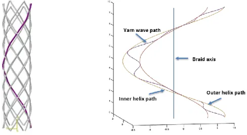
A Python script was programmed to parametrize and automate the generation of the model into the commercial FEM software ABAQUS. The script generates the nodes following yarn paths of a cylindrical bi-axial braids with user-defined properties. As shown in Figure 1, the braiding yarns track a periodic oscillating path between two parallel helical curves.

Figure 1: Braided yarn geometrical modeling features

:

The helices make a complete turn around the braid axis for one braid pitch. The helical equations bounding the yarn path can be considered as,

(1)

Where xin, yin, xout ,yout and z are the helices positions in the tree-dimensional Cartesian coordinates. Here, the subscripts ‘in’ and ‘out’ are used to denote the inner and outer helices between which the braided yarn oscillates. D is the braid diameter, ψ is the helical angle which 0<ψ<2π for a complete helix, P is the braid pitch and λ is the coefficient to characterize the yarn direction, if λ=1 yarns move in the clockwise and when λ= -1 yarns move in the counter-clockwise direction. While one set of braiding yarns are helically wrap around the braid, another set move in the opposite direction by crossing over and under the yarns. The braided yarn oscillating path is defined using the following equations,

𝑋

_𝑐

= 𝑥

_𝑖𝑛

+ 𝑥

_𝑣

𝐿 (1 + cos

2𝜋(𝑖−1)_𝑛

), 𝑌

_𝑐

= 𝑦

_𝑖𝑛

+ 𝑦

_𝑣

𝐿 (1 + cos

2𝜋(𝑖−1)_𝑛

), 𝑍

_𝑐

= 𝑧

with,

𝑥

_𝑣

= 𝑥

_𝑜𝑢𝑡

− 𝑥

_𝑖𝑛

, 𝑦

_𝑣

= 𝑦

_𝑜𝑢𝑡

− 𝑦

_𝑖𝑛

, 𝐿 = √𝑥

_𝑣2

_{+ 𝑦}

𝑣2 (2)      2 , sin 2 , cos 2 , sin 2 , cos 2 P z D y D x D y D x out out out out in in in in           2 , sin 2 , cos 2 , sin 2 , cos 2 P z D y D x D y D x out out out out in in in in           2 , sin 2 , cos 2 , sin 2 , cos 2 P z D y D x D y D x out out out out in in in in           2 , sin 2 , cos 2 , sin 2 , cos 2 P z D y D x D y D x out out out out in in in in           2 , sin 2 , cos 2 , sin 2 , cos 2 P z D y D x D y D x out out out out in in in in     

(5)

4

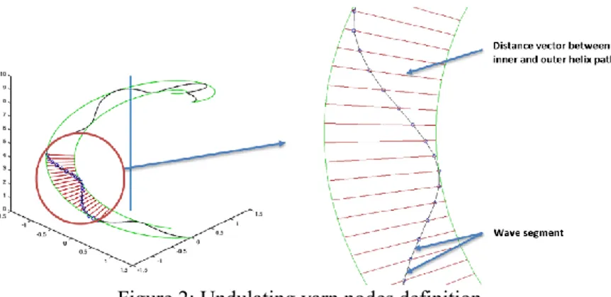
Where xv and yv and z are the vector coordinates of the shortest distances between outer and inner helix circles. These shortest distance line segments are laying on planes perpendicular to the braid axis defined at each z. Xc, Yc and Zc are points defined on each shortest distance line segments. They define the yarn node positions during a cosine wave where n is the number of wave segment and i=1 to n+1. For the FEM meshing, each segment is automatically attributed an element along the fiber path. Figure 2 presents the yarn node positions and yarn segments.

Figure 2: Undulating yarn nodes definition

The yarn cross-sections are assumed to be circular with constant diameter. The fibers are assembled as a concentric layer of circles packed into a yarn. The Python script automatically generates the fibers through a circle packing algorithm. The diameter of fibers is varying depending on the amount of fibers inside a yarn. Different yarn fibering examples are shown in Figure 3.

(a) (b) (c)

Figure 3: Circular packing of fibers in the braided yarn. (a) Yarn contains 7 fibers; (b) Yarn contains 19 fibers; (c) Yarn contains 37 fibers.

For demonstration and validation purposes, a braid containing 12 yarns was selected. The geometrical properties of the selected braid are presented in Table 1.

Yarn radius (m) Pitch length

(m) Din (m) Dout (m)

3.9088E-4 0.02 0.005 0.0066

Table 1: Selected bi-axial braid geometrical properties.

2.2 Mesh generation

Three-dimensional solid beam elements with circular cross-section are assigned along a fiber. Beam elements are Timoshenko beams (shear flexible) with two-node linear interpolation formulations. Six degrees of freedom, three translational and three rotational motion, are active for each node in three-dimensional space. To simulate the fiber’s flexibility, elements are joined together at their two end nodes. Therefore, the end-to-end connected nodes share their

(6)

5

translational and rotational degrees of freedom. Each yarn is modeled as the bundle of beam elements inside the braid. The beams can suffer different mechanical loads such as tension and compression along the element axis, bending perpendicular to the element axis, shear transverse to the element axis and torsion parallel to the axis of beam element. All beam elements have equal length. The aspect ratio (c=le/de) varies depending on the number of fibers per yarn and elements per fiber.

2.3 Contact simulation

The fibers interactions are modeled by ABAQUS/Explicit general contact algorithm. This algorithm allows to detect many contact regions automatically and is appropriate for beam-to-beam contacts and complex topology. In addition, general contact is considerably faster than other contact algorithms in ABAQUS. After contact detection, there is no penetration observed between the contacted beams. The mechanical tangential and normal behavior are defined for contact properties. Penalty friction formulation is selected with a friction coefficient of 0.3, no limit shear stress and infinite elastic slip stiffness for mechanical tangential behavior. To minimize the penetration between touching fibers, the “hard” contact is used in the pressure-overclosure relationship for the contact mechanical normal behavior.

2.4 Material properties

Carbon fibers are anisotropic materials. It should be noted that isotropy is taken as the main assumption for material properties of beam elements, there is no anisotropy characteristics of beam elements in ABAQUS software. Therefore, isotropic elastic material properties are considered for the carbon fibers material. The material properties of carbon fibers assigned for fibers model are presented in Table 2.

E (GPa) 230

ρ (Kg/m3₎ ₁₇₅₀

ν 0.22

Table 2: Material properties applied to beam fiber elements.

2.5 Boundary conditions and loading rate

Only the axial translational movement is fixed on the last node of each fiber. These nodes are allowed to translate and rotate in all other directions. Also, axial tensions are smoothly applied on the fiber nodes of the other end of the braid. In a quasi-static solution, immediate loading may lead to the propagation of a stress wave through the model and generate noisy and inaccurate solution. Ramping up the loading gradually from zero removes this detrimental effect. In order to increase accuracy and efficiency, the model requires the use of tension forces as smooth as possible. Therefore, the quasi-static procedure is upgraded by applying loads gradually using a smooth loading curve.

2.6 Speed up the simulation: Mass scaling

The textile FEM consumes time to detect contact between fibers. This has a detrimental effect on the total computing time. Moreover, increasing the number of fibers per yarn inside the model increase the computing cost. For example, the single layer of braid model with 37 fibers assembled in each yarn requires more than one week running on a system using four 3.00 GHz cores. Therefore, the mass scaling technique may be used to achieve a reasonably economical computing time. Impressive computing time is saved in quasi-static procedure using the mass scaling technique. In quasi-static explicit analysis, increasing the stable time increment (∆t) leads to a reduction in computing cost. The stable increment time was estimated by the following relations,

(7)

6

,

(3)

Where Le_{is the smallest characteristic element length, c}

d is the dilatational wave speed of the material, E is the young modulus and ρ is the material density. Clearly increasing the material density causes to increase the stable time increment and finally reduce the total computing time. According to above relations, if the material density is artificially increased by a factor of f 2_{, the stable increment time will be increased by factor of f. Table 3 compares} the computer run time of the braid model with 37 fibers assembled in each yarn with different mass scaling factor. It is obvious that increasing the density by mass scaling reduces the CPU time. However, this technique may yield inaccurate reliable results if excessive mass scaling is employed.

f Computing time

1 8 days

1E3 11 h

10E3 93 min

1E6 14 min

Table 3: Computing time with different mass scaling factor.

2.6.1 Mass scaling evaluation using energy balance

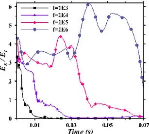
Using a high level of mass scaling increase the kinetic energy can lead to wrong results. To ensure that successful implementation of mass scaling and keep quasi-static simulation, the kinetic energy must be a small fraction (less than 5%) of strain energy [18]. The Figure 4 shows the ratio of kinetic energy (EK)-to-internal energy (EI) along the simulation time of the models which are evaluated for different mass scaling factors associated with the values of Table 3. The mass scaling evaluation has shown that for a mass scaling factor more than 10,000, the kinetic energy is high in comparison to the internal energy during the analysis. Therefore, they cannot be considered as a quasi-static procedure for these mass scaling values. Hence, the mass scale with factor of 10,000 is considered for all analyses.

Figure 4: Comparison ratio of kinetic energy (EK)-to-internal energy (EI)

for different mass scaling factor (f=1E3, f=1E4, f=1E5, f=1E6).

d e

c

L

t







E

c

_d



(8)

7

2.7 Convergence and accuracy studies

Since the simulation with a great number of fibers, i.e. 12K yarn, is impossible, the sufficient number of fibers per yarn must be determined for fabric modeling. Models containing 7, 19, 37 and 61 fibers per yarn were simulated to study the convergence of the model to reproduce an accurate braid structure. The deformed cross-sections of these models at an arbitrary coordinate of z = 0.02 m are shown in Figure 5. The cross-section figures demonstrate that the yarn with more fibers predicted yarn configuration more accurately while extremely increasing the computing time. Therefore, using 19 fibers per yarn has provided a reasonable analysis without leading to unmanageable computing time. The yarn cross-sections in Figure 5b to d have similar geometries. Therefore, it can be said that geometrical convergence was reached by using 19 fibers per yarns. The small fibers penetration can be seen in some neighboring fibers even if no error was reported during simulation. The model requires some contact modifications to remove these unwanted penetrations.

a) b) c) d)

Figure 5: The braid cross-section comparison. Each yarn contains 7 fibers. b) Each yarn contains 19 fibers. c) Each yarn contains 37 fibers. d) Each yarn contains 64 fibers.

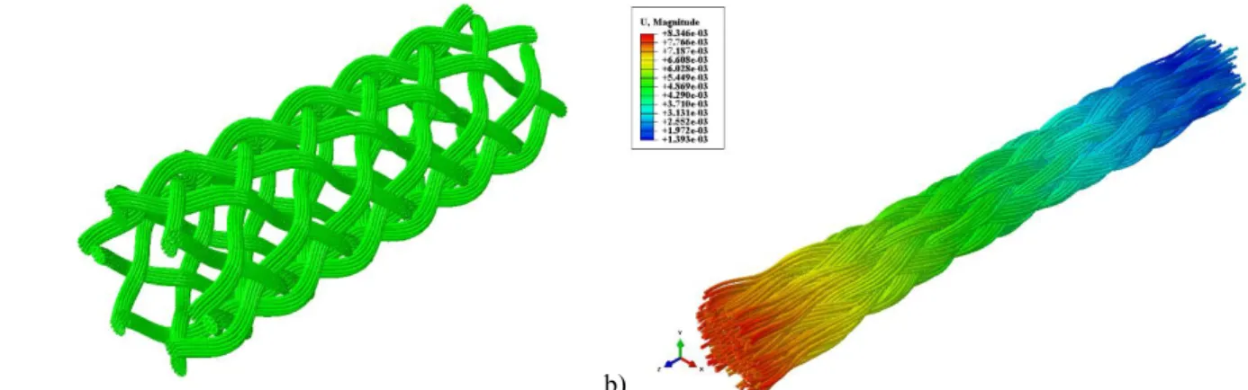
The un-deformed and deformed braid model configuration with 19 fibers assembled in each yarn is shown in Figure 6.

a) b)

(9)

8

3 EXPERIMENT

3.1 Braid manufacturing and CT-scanning

A carbon fiber braid was manufactured by 24 carrier braiding machine and 12K carbon yarns. 12 yarns were used to produce the bi-axial diamond (1/1) braid pattern. A specimen of carbon braid was cut to assess the internal structure of the braid and compare with the model using micro CT-scanning (XT H 225, Nikon). To hold the braid specimen and applying in-situ axial tension on it during the CT-scanning, a fixture mechanism was designed and assembled comprising an acrylic tube, two caps and eyebolts and nuts as shown at Figure 7. The braid specimen was located concentrically inside the acrylic tube while the two ends of the specimen were tied to the eyebolts. Tightening the nuts allowed to apply the suitable in situ axial tension on the braid specimen simultaneously with micro CT-scanning. The micro structure, internal architecture and cross-sectional view of the braid can be observed after the micro CT-scanning.

a) _b)

Figure 7: The acrylic tubed fixture. a) The schematic image. b) Fixture installed on the CT -scan holder.

3.2 Results validation

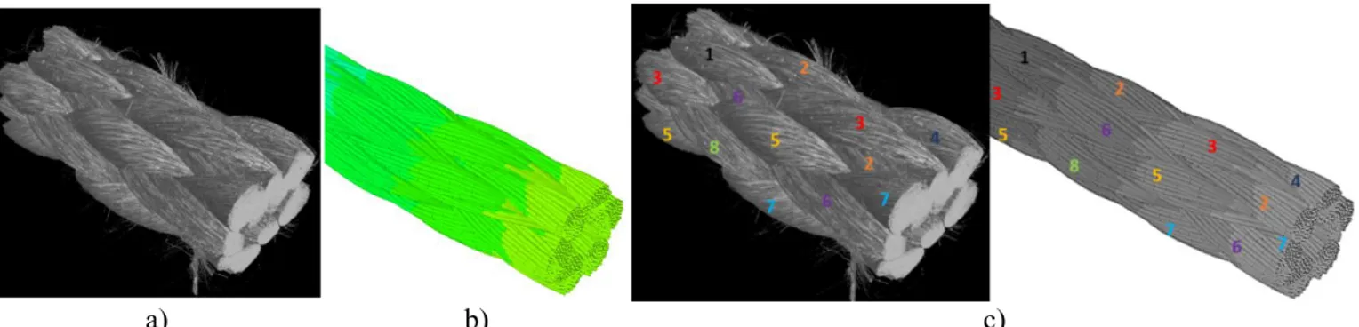
Figure 8 shows the results of simulations compared with the 3D micro CT scan of the real carbon braid specimen. There is an excellent agreement of the model results with the real carbon braid. Yarn by yarn comparison between CT image and model is shown at Figure 8c.

a) b) c)

Figure 8: Comparison results. a) 3D CT image of carbon braid. b) Braid model. c) Correspondence of yarn numbering on CT-Scan and braid model.

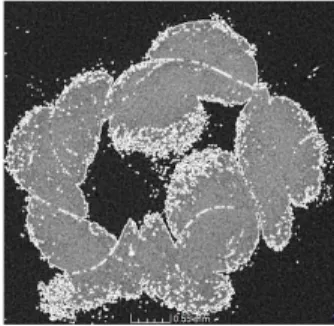
Also, the model accurately predicts the hollow center of braid as shown in Figure 9. The model cross-section always remains circular in shape but the specimen cross-section is deformed. This deformation is attributed to the braid

(10)

9

attachment fixture. Nevertheless, the yarns cross-sections in the left-side of the real braid tend to correspond to the model.

Figure 9: Comparison of the braid cross-sections. a) CT scan cross-section image. b) Braid model cross-section.

4 CONCLUSION

A braid model at fiber level/micro scale was presented. Each yarn of braid is modeled as a bundle of 3-D Timoshenko beam elements using Python scripting in commercial FE software ABAQUS/Explicit. ABAQUS/Explicit general contact algorithm was used to model the fiber-to-fiber (beam-to-beam) interactions. An effective computing time was saved in quasi-static procedure by the mass scaling technique. The mass scaling factor of 10 000 reduced the computing time from 8 days to 93 minutes without generating kinetic energy levels outside the quasi-static assumption. To validate the method, a specimen of braided carbon fiber was prepared for micro CT scanning. Comparing the CT images with the primary results obtained from the model reveals that the model predicts the behavior of the fiber structure with a reasonable tolerance. The presented method could accurately determine fiber position in braided structures by considering the fiber to fiber interactions. The effect of the friction coefficient, elasticity modulus, linear and quadratic elements on the model will be investigated. The model will be used for the analysis of the various steps of manufacturing of thermoplastic composite braided rod. Moreover, the method will be able to model other types of fabric reinforced composites.

5 ACKNOWLEGEMENTS

The authors would like to thank Bombardier Aerospace, Pultrusion Technique, NSERC

(CRDPJ488387-15) and Prima Quebec for financing this research project.

6 REFERENCES

[1] Wiedmer, S. and M. Manolesos, An experimental study of the pultrusion of carbon fiber-polyamide 12 yarn. Journal of Thermoplastic Composite Materials, 2006. 19(1): p. 97-112.

[2] Michaeli, W. and D. Juerss, Thermoplastic pull-braiding: pultrusion of profiles with braided fiber lay-up and thermoplastic matrix system (PP). Composites Part A: Applied Science and Manufacturing, 1996. 27(1): p. 3-7.

[3] Bechtold, G., et al. Pullbraiding of commingled GF/PP yarn: influence of processing parameters. in Proceedings 4th International Symposium for Textile Composites (TexComp). 1998. Kyoto, Japan.

[4] Lebel, L.L. and A. Nakai. Design and Manufacturing of an L-Shaped Thermoplastic Composite Beam by Braid-Trusion.

(11)

10

[5] Y. Wang and X. Sun, "Digital-element simulation of textile processes," Composite Science and Technology, vol. 61, pp. 311-319, 2001.

[6] G. Zhou, X. Sun, and Y. Wang, "Multi-chain digital element analysis in textile mechanics," Composites Science and

Technology, vol. 64, pp. 239-244, 2004.

[7] Y. Miao, E. Zhou, Y. Wang, and B. A. Cheeseman, "Mechanics of textile composites: Micro-geometry," Composites

Science and Technology, vol. 68, pp. 1671-1678, 2008.

[8] L. Huang, Y. Wang, Y. Miao, D. Swenson, Y. Ma, and C.-F. Yen, "Dynamic relaxation approach with periodic boundary conditions in determining the 3-D woven textile micro-geometry," Composite Structures, vol. 106, pp. 417-425, 2013. [9] D. Durville, "Simulation of the mechanical behaviour of woven fabrics at the scale of fibers," International Journal of

Material Forming, vol. 3, pp. 1241-1251, 2010.

[10] D. Durville, "Contact-friction modeling within elastic beam assemblies: an application to knot tightening," Computational

Mechanics, vol. 49, pp. 687-707, 2012.

[11] T. D. Vu, D. Durville, and P. Davies, "Finite element simulation of the mechanical behavior of synthetic braided ropes and validation on a tensile test," International Journal of Solids and Structures, vol. 58, pp. 106-116, 2015.

[12] Y. Mahadik and S. R. Hallett, "Finite element modeling of tow geometry in 3D woven fabrics," Composites Part A:

Applied Science and Manufacturing, vol. 41, pp. 1192-1200, 2010.

[13] S. D. Green, A. C. Long, B. S. F. El Said, and S. R. Hallett, "Numerical modeling of 3D woven preform deformations,"

Composite Structures, vol. 108, pp. 747-756, 2014.

[14] texgen.sourceforge.net/index.php/Main_Page

[15] R. Samadi and F. Robitaille, "Particle-based modeling of the compaction of fiber yarns and woven textiles," Textile

Research Journal, vol. 84, pp. 1159-1173, 2014.

[16] N. Metropolis, A. W. Rosenbluth, M. N. Rosenbluth, A. H. Teller, and E. Teller, "Equation of state calculations by fast computing machines," The journal of chemical physics, vol. 21, pp. 1087-1092, 1953.

[17] Y. Crama and P. L. Hammer, Boolean functions: Theory, algorithms, and applications: Cambridge University Press, 2011.

[18] A. Prior, "Applications of implicit and explicit finite element techniques to metal forming," Journal of Materials