HAL Id: hal-00862364
https://hal.archives-ouvertes.fr/hal-00862364
Submitted on 16 Sep 2013
HAL is a multi-disciplinary open access
archive for the deposit and dissemination of
sci-entific research documents, whether they are
pub-lished or not. The documents may come from
teaching and research institutions in France or
abroad, or from public or private research centers.
L’archive ouverte pluridisciplinaire HAL, est
destinée au dépôt et à la diffusion de documents
scientifiques de niveau recherche, publiés ou non,
émanant des établissements d’enseignement et de
recherche français ou étrangers, des laboratoires
publics ou privés.
Extension of the transmission line theory application
with modified enhanced per-unit-length parameters
Sofiane Chabane, Philippe Besnier, Marco Klingler
To cite this version:
Sofiane Chabane, Philippe Besnier, Marco Klingler. Extension of the transmission line theory
appli-cation with modified enhanced per-unit-length parameters. Progress In Electromagnetics Research,
2013, 32, pp.257. �10.2528/PIERM13072308�. �hal-00862364�
1
EXTENSION OF THE TRANSMISSION LINE
THEORY APPLICATION WITH MODIFIED
ENHANCED PER-UNIT-LENGTH
PARAMETERS
S. Chabane1, P. Besnier1 and M. Klingler2
1 IETR: Institute of Electronics and Telecommunications of Rennes, CNRS UMR 6164, INSA of Rennes,
20 av. des Buttes de Coësmes, CS 14315, Rennes Cedex 35043, France E-mail: sofiane.chabane@insa-rennes.fr
2 PSA Peugeot-Citroën, Centre Technique de Vélizy, 2 route de Gisy, 78943 Vélizy-Villacoublay Cedex,
France
E-mail: marco.klingler@mpsa.com
Abstract- This paper introduces a modified enhanced transmission-line theory to account for higher-order
modes while using a standard transmission line equation solver or equivalently a Baum, Liu and Tesche (BLT) equation solver. The complex per-unit-length parameters as defined by Nitsch et al. are first cast into an appropriate per-unit-length resistance, inductance, capacitance and conductance (RLCG) form. Besides, these per-unit-length parameters are modified to account for radiation losses with reasonable approximations. This modification is introduced by an additional per-unit-length resistance. The reason and explanations for this parameter are provided. Results obtained with this new formalism are comparable to those obtained using an electromagnetic full-wave solver, thus extending the capability of conventional transmission line solvers.
1. INTRODUCTION
Complex systems such as automobiles or other vehicles have to meet electromagnetic compatibility (EMC) requirements. Design engineers need to predict the performances of their products in the early stage of their development. EMC simulation tools should be able to help developers to analyze the EMC performances of the vehicle and its electrical and electronic architecture.
The most vulnerable point of a vehicle is its equipment, since faults caused to the equipment modules may lead to various types of malfunctions. These faults may be the consequence of the induced currents and voltages on the wires of the harnesses. The electromagnetic interference calculations at the end of harness networks are still a challenge for many equipment modules or systems. Topology of harnesses and the important number of individual wires is one obvious reason for this.
Hopefully, given the relative proximity of wires to the surrounding large metallic or conducting structures, the transmission line theory (TLT) is applied in most cases. It thus reduces the complexity and the cost of calculations. Using the field to transmission line (TL) coupling formalism such as Agrawal’s model [1], it is possible to split calculations into two decoupled problems. First, the field calculation along the routes of the harnesses in absence of the wiring is performed by the means of a 3D Maxwell’s equation solver. Then, a multi-conductor transmission line solver is used to calculate currents and voltages induced on the wires, using the field values calculated in the first step.
However, TLT is limited by some assumptions that are not always under control and cannot always be used. Indeed, the classical TLT equations can easily be derived from Maxwell's equations after approximating the Green’s function relating the sources (incident electromagnetic field) to the reaction of the wire (induced currents and voltages) [2]. The main assumption is that the distance between the TL and its return path should be much smaller than the minimum considered wavelength of the current flowing in it. As a consequence of this simplification, the result of the Green's function integral along the TL contains no imaginary part, i.e. the radiation resistance is altogether neglected and the wave is considered totally guided along the TL.
Nevertheless, there are some situations for which this approximation may not stand. Obviously, it’s difficult to establish a definite limit of the separation distance that must not be exceeded unless one imposes an
2
arbitrary criterion. Moreover, this approximation may yield to inaccurate current estimations at the resonance frequencies, since in this case the radiation resistance may play an important role.
For these reasons, extending the ability of the TLT to handle higher order modes while keeping the simplicity of its formalism would be a significant improvement.
Numerous advanced studies have met some success in this direction. Some new models have been directly derived from Maxwell’s equations without the height limitation. However, most of these models are based on iterative time- and memory-consuming solutions, and are rather suitable either for mono conductor situations [3] or for short conductors such as the interconnects [4].
The more general and rigorous formalism is the one known as the transmission line super theory [5]. This theory presents a rigorous derivation of Maxwell's equations for non-uniform transmission lines into a set of coupled equations which resembles the telegrapher's equations. The per-unit-length (p.u.l.) parameters, which are position- and frequency-dependent, are calculated through a rather complex iterative procedure. Besides, the computation of the solution of these equations remains cumbersome and needs an entire new software development.
The enhanced transmission line p.u.l. parameters defined in [6] allow taking into account higher-order modes for uniform transmission lines using a rigorous derivation of the integral of the Green's function. However, these enhanced p.u.l. parameters cannot directly be used in a TLT solver (like the Baum, Liu and Tesche (BLT) equation-based solver [7, 8]) and therefore require an entire new software development.
The purpose of this paper is, on the one hand, to derive a proper representation of these parameters easy to embed in a classical TL solver or in its BLT form solver and, on the other hand, to show how the energy related to the radiation is dissipated. Indeed, putting the complex p.u.l. parameters defined in [6] under a resistance, inductance, capacitance, conductance (RLCG) form leads only to the decomposition of the modes in terms of TEM modes supported by the real part of the characteristic impedance, and radiating modes (or antenna mode) supported by the imaginary part of the characteristic impedance. Therefore, in this paper we will also present a modified version of these enhanced parameters that will converge to the solution of the differential currents at the ends of the TL. This solution allows calculating these currents using a classical BLT solver with a good approximation, even at critical resonant frequencies or when the conditions of application of the classical TLT are not fulfilled. In this paper, we present and validate this method for a single wire above a perfect ground plane.
2. ENHANCED TRANSMISSION-LINE THEORY
Let us consider a lossless TL above a perfectly conducting (PEC) ground plane in presence of an external electromagnetic field as shown in figure 1.
From Maxwell's equations, and using the thin wire approximation, the field-to-transmission line coupling equations are given by [2]:
) z , h ( E ) ' z ( d ) ' z ( I ) ' z z ( g j dz ) z ( dV e z L s
0 0 4 (1) 0 4 0 0
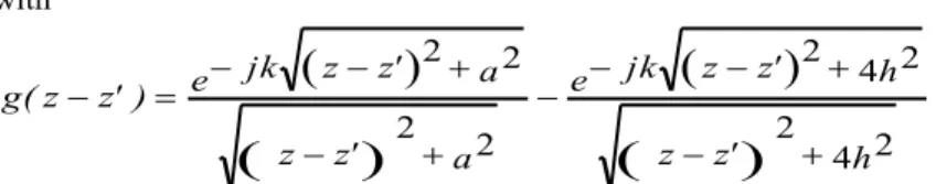
g(z z' )I(z' )dz' j Vs(z) dz d L (2)3 with
z z'
h e jk z z' h a ' z z e jk z z' a ) ' z z ( g 4 2 2 4 2 2 2 2 2 2 (3) ) z (Vs represents the scattered voltage as defined in the classical TLT [1, 2], I(z' )is the current amplitude, )
z , h (
Eze is the incident tangential electric field, zand z'stand respectively for the position of the observation point and the source points to the origin, and g(zz' )is the Green's function of this configuration.
Figure 1. Geometry of the studied problem
Thus, considering the observation point being far enough from the ends of the wire and the current locally constant, the integral limits can be taken from to and the current distribution placed out the integral [2]. Then, from [6] and using some Bessel functions properties, we can easily find:
Y hk Y ak
j
J
hk J
ak
' dz ) ' z z ( g 0 2 0 0 2 0 (4) Here J0 and Y0are, respectively, the 0-order Bessel functions of first and second kind.Now, using the expansion form of Y0 as given in [9]:
1
1
1
2
2
2
1
2
0
2
2
0
k
k
m
m
!
k
z
k
k
)
(
z
J
z
ln
)
z
(
Y
(5)and after some rearrangements the above integral (4) can be rewritten as:
j
J
hk
J
ak
k
m
m
k
k
!
k
ak
k
k
m
m
k
k
!
k
hk
k
ak
J
ak
ln
hk
J
hk
ln
a
h
ln
'
dz
)
'
z
z
(
g
0
2
0
1
1
1
2
2
2
1
1
1
1
2
2
1
2
1
0
2
1
2
0
2
2
2
(6)The classical approximation for this integral consists in assuming that all terms are negligible with respect to the first one on the right-hand side of (6). In the following these terms are considered as a correction factor. Hereafter, we express the real part of this correction factor as:
4
k m k k k k m k k k F m ! k ak m ! k hk ak J ak ln hk J hk ln C 1 1 2 2 1 1 2 2 0 0 1 2 1 1 1 2 1 2 1 2 2 (7)and the imaginary part as:
CF
J0
2hk J0
ak
(8) Using these definitions and substituting them in (1) and (2), we get:
j L R
E (h,z) ) z ( I dz ) z ( dV e z HF HF s (9)
0 Vs(z)j CHF GHF dz ) z ( dI (10) where the explicit forms of these p.u.l. parameters are given by:
F ' HF L C L 4 0 0 (11)
F HF C R 4 0 (12)
a h ln C C a h ln C a h ln C a h ln C C F F F F ' HF 2 2 2 4 2 4 2 2 2 2 2 0 (13)
a h ln C C a h ln C a h ln C C G F F F F ' HF 2 2 2 4 2 4 2 2 2 0 (14)and where the classical p.u.l. parameters are given by: a h ln L' 2 2 0 0 (15) and a h ln C' 2 2 0 0 (16)
Note that (9) and (10) have exactly the same form as the classical ones. Hence, to solve this system all the known methods of resolution in the classical case can be used here. In our case, we use the BLT formulation of the TL equations.
Besides, the new enhanced p.u.l. parameters are now frequency-dependent and are not limited to the quasi-static approximation but reduced to the classical ones where the classical TLT assumptions are fulfilled.
The resistance and the (negative) conductance parameters account for higher-order modes whereas the frequency-dependent inductance and capacitance can differ significantly from the classical ones, especially when the quasi-static approximation is no longer valid.
Since the p.u.l. parameters are enhanced and become frequency-dependent, we can expect that the characteristic impedance is also frequency-dependent.
From (4), (1) and (2), we find that the enhanced p.u.l. impedance is given by:
Y hk Y ak j J hk J ak
j z 02 0 0 2 0 4 0
(17) The enhanced per-unit-length admittance is written as:5
Y hk Y ak
j
J
hk J ak
j y 0 0 0 0 0 2 2 4 (18) Using the classical definition of the characteristic impedance as the square root of the ratio between the impedance and the admittance:y z
Zc (19) It can easily be proven that the enhanced characteristic impedance is complex and is given by:
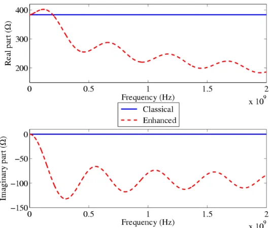
Y hk Y ak j J hk J ak
Zc 0 0 0 0 0 0 2 2 4 1 (20) Thus, the characteristic impedance, even for a lossless transmission line, becomes complex and frequency-dependent (fig. 2).Figure 2. Comparison between the classical and enhanced characteristic impedance for a lossless TL above a PEC ground, height=0.3m, radius=1mm.
Now, we investigate the effect of the enhanced p.u.l. parameters on the propagation constant. The propagation constant, in its general form is given by:
j (21) where
and
are, respectively, the attenuation and phase constants.The propagation constant is calculated through:
2 ZY RHF jLHF GHF jCHF (22) Replacing ZY in (22) by (17) and (18), we get:
0 0 2 2
(23) Since the result of the product is a pure negative real value, the propagation constant is a pure imaginary term. This means that the use of these new p.u.l. parameters will not lead to energy dissipation. In other words, the energy is still stored in the TL. Nevertheless, these enhanced parameters allow to split the energy propagating on the TL into TEM and radiated modes as shown below.
6 Indeed, (19) can also be written as:
HF HF HF HF c C j G L j R Z (24) Considering that GHFCHF and using (8), (12) and (20) we can easily get:
k R j C L Z HF HF HF c (25)
The energy of the TEM mode is related to the real part of the characteristic impedance whereas the energy of the radiated mode is related to the imaginary part.
3. MODIFIED-ENHANCED P.U.L PARAMETERS
As shown above, the enhanced p.u.l. parameters lead only to the separation of the TEM mode and radiated mode on a TL. It means that the currents and voltages at the ends of the TL are not affected and using these enhanced parameters does not provide more accurate results. In order to dissipate the radiated energy, a possible method is to calculate appropriate reflection coefficients at the ends of the TL [2]. We rather introduce a more convenient and new method that consists in adding another p.u.l. resistance that will be related to the radiated energy.
This additional resistance
R
is inserted in series with RHF and LHF. The following developments present the theory related to this additional resistance in the case of a single wire above a ground plane.Since an additional resistance
R
is introduced, the attenuation constant
is non-null.The wave attenuation factor for the square of the current (or of the voltage) over the length
L
of the TL can be written as:) L exp( ) L ( A 2 (26)
The power to be radiated can be associated with the ratio between the imaginary part and the real part of the characteristic impedance, which is shown, in the following, to be equivalent to the definition of the quality factor Q of the TL.
From (25) this Q factor can easily be written as:
HF HF HF HF HF line R L C L R Q (27)
When an additional resistance
R
is added to the p.u.l. parameters, (22) becomes:
2 RHF R jLHF GHF jCHF (28)
Considering the property RHFCHF LHFGHF and after rearrangement, we get:
2 RHF RGHF LHFCHF 2 jRCHF (29)
In the following, we assume that
RHFR
GHF LHFCHF2. Nevertheless, this assumption will be verifieda posteriori. It must be noted that this condition is also equivalent to:
22 HF HF
HF R R L
R (30)
If this assumption is fulfilled, then 2 can be approximated as: 2 LHFCHF 2 jRCHF (31)
Since
j
, it follows that: 2 2 2 2 2 2 1 2 HF HF HF HF HF L R C L C L (32)
The second term under the square root is verified to be much smaller than one. Then, a first order series expansion can be used to extract 2:
7
HF HF L C R 4 2 2 (33)Using the definition of the attenuation factor in (26), (27) and (33), we find that the attenuation on the TL introduced by R is equal to:
HF HF HF HF L R L L C R exp ) L ( A ) ( A 1 0 (34)
In order to determine R, this attenuation is identified with the inverse of the Q factor of the TL. Finally, we obtain: L R L R ln C L L R HF HF HF HF HF 1 1 (35)
As expected, the p.u.l. additional resistance is equivalent to the imaginary part of the characteristic impedance (25) distributed along the TL and is frequency-dependent (fig. 3a). Besides, this additional resistance does neither affect the phase constant nor the characteristic impedance but only the attenuation constant (fig. 3b). This is due to the fact that it is relatively small compared to the p.u.l. resistance (35).
(a) The additional correction resistance.
(b) Characteristic impedance and propagation constant.
Figure 3. Characteristics of the modified enhanced p.u.l. parameters for a lossless TL above a PEC ground, height=0.3m, radius=1mm.
8
4. RESULTS
In order to validate this new model, some simulations have been carried out. The p.u.l. parameters are calculated either using their classical form or using their modified enhanced version presented previously. They are inserted in a BLT equation solver. Both results are compared to those obtained with an electromagnetic full-wave method of moments (MoM) solver (FEKO). The current in the load is calculated as a function of the frequency of the excitation signal. Though the p.u.l. parameters, the associated characteristic impedance and the propagation constant were calculated up to 2GHz, in the following the currents will be calculated only up to 500MHz to keep the clarity of the figures.
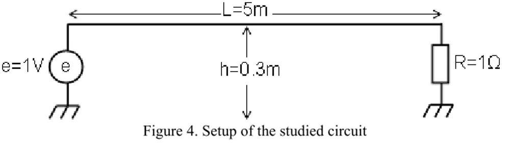
The configuration studied is presented in Fig. 4. It consists in a perfectly conducting and non-coated wire of 5m length and 1mm radius at 30cm above a perfectly conducting ground plane. It is fed by a sinusoidal voltage source e of 1V at one end and loaded with a resistance R of 1 at the other end.
Figure 4. Setup of the studied circuit
Fig.5 shows the current that flows in the resistance calculated from three different methods. The black curve is calculated with the classical TL equations. It highlights that the resonance levels are quite high and their amplitude does not follow a regular pattern since they depend strongly on the frequency sampling points. Since no losses are taken into account, the highest peak level is expected to be 0 dBA. The green curve shows the result of our modified enhanced version of the TL solver. The level of the resonances follow a much more regular evolution with frequency and calculations predict much lower peak levels as expected. For comparison, the calculation performed with the MoM solver is presented in red.
Below roughly 300 MHz, results obtained with our model are in good agreement with the full-wave solver. Beyond this frequency, the modified enhanced model does not provide results in agreement with the MoM calculations. This can be explained by the effect of the vertical wires that are only modeled in the full-wave solver (for practical reasons) and not in the TL approach. The effect of these vertical wires can be approximately taken into account through the addition of a p.u.l. resistance of these wires calculated from the radiation resistance of a monopole antenna [10, 11]. As expected (Fig. 6), this produces slightly better results (5 dB beyond 400 MHz). However, even with this correction, if we compare to the MoM results in fig. 5, there are still some differences higher in frequency. This is due to the monopole model used for the vertical wires and possibly to the effect of the coupling between the horizontal and vertical wires. Nevertheless, in real cases, wires are not perfect conductors and as a consequence, the amplitudes of the current induced in the loads are even lower than predicted by the results in Fig. 5 and 6. Therefore, the proposed model leads to responses much more realistic than the classical TLT model, and provides, in general, a better approximation especially for the most critical first resonances.
9
Figure 5. Current amplitude as a function of the frequency at the end of the TL, using the modified enhanced p.u.l. parameters.
Figure 6. Current amplitude as a function of the frequency at the end of the TL, using the modified enhanced p.u.l. parameters and including the vertical wires.
10
5. CONCLUSIONS
In this letter, we have presented a modification to the enhanced per-unit-length (p.u.l.) parameters of a single transmission line (TL) which were first explicitly extracted from [6]. This modification was necessary since the enhanced parameters only enable to split the energy propagating on the TL into TEM and radiated modes. Thus, to dissipate energy, an innovative solution has been demonstrated which consists in adding a supplementary p.u.l. resistance to the enhanced p.u.l. resistance and inductance. This additional p.u.l. resistance corresponds approximately to the imaginary part of the characteristic impedance of the TL. The results obtained are comparable to those obtained with a full-wave software even at resonant frequencies. This new formalism is currently being generalized to take into account multi-conductor configurations and coated wires.
AKNOWLEDGMENT
This work is sponsored by the French CNRS and PSA Peugeot-Citroën.
References
1. Agrawal, A. K., Price, H. J. and Gurbaxani, S. H.: ‘Transient response of a multiconductor transmission tine excited by a nonuniform electromagnetic field,’ IEEE Trans. Electromagn. Compat., vol. EMC-22, No 2, pp. 119-129, May 1980.
2. Rachidi, S.V, and Tkachenko, V.S. :’Electromagnetic field interaction with transmission lines. From classical theory to HF radiation effects’, WITpress, 2007.
3. Tkachenko, S.V., Rachidi, F. and Ianoz, M., "Electromagnetic Field Coupling to a Line of Finite Length: Theory and Fast Iterative Solutions in Frequency and Time Domains", IEEE Trans. on Electromagn. Compat., vol. 37 No 4, pp.509-518, Nov. 1995.
4. Maffucci, A., Miano, G. and Villone F., "An Enhanced Transmission Line Model for Conducting Wires", IEEE Transactions on Electromagnetic Compatibility, Vol. 46 No 4, pp. 512-528, Nov. 2004.
5. Nitsch, J., Gronwald, F. and Wollenberg, G., Radiating Nonunifrom Transmission-Line Systems and the Partial Element Equivalent Circuit Method: John Wiley & Sons, 2009.
6. Nitsch, B. J., and Tkachenko, V. S.: ‘Complex-valued transmission-line parameters and their relation to the radiation resistance’, IEEE Trans. Electromagn. Compat., vol. 46, No 3, pp. 477-487, Aug. 2004.
7. Baum, C.E., Liu, T.K., and Tesche, F.: ‘On the analysis of general multiconductor transmission line networks’, Interaction Notes 350, Kirtland,AFB, NM, Nov. 1978.
8. Parmantier, J. P. and Degauque, P.: ’Topology-based modeling of very large systems’, in Modern Radio Science, J. Hamelin, Ed. London, U.K.: Oxford Univ. Press, pp. 151–177, 1996.
9. Watson, G.N.,: ‘A treatise on the theory of Bessel functions’, Cambridge University Press, 1922.
10. Schelkunoff, S.A, and Friis, H.T. :’Antennas - theory and practice’, New York, John Wiley & Sons, Inc., 1952.
11. Pignari, S. A., and Bellan, D.: ‘Incorporating vertical risers in the transmission line equations with external sources’, Proc. Int. Symp. on Electromagn. Compat., vol. 3, pp. 974-979, Aug. 9-13, 2004.