HAL Id: hal-01021210
https://hal.inria.fr/hal-01021210
Submitted on 9 Jul 2014HAL is a multi-disciplinary open access archive for the deposit and dissemination of sci-entific research documents, whether they are pub-lished or not. The documents may come from teaching and research institutions in France or abroad, or from public or private research centers.
L’archive ouverte pluridisciplinaire HAL, est destinée au dépôt et à la diffusion de documents scientifiques de niveau recherche, publiés ou non, émanant des établissements d’enseignement et de recherche français ou étrangers, des laboratoires publics ou privés.
Bayesian Updating of Probabilistic Time-Dependent
Fatigue Model: Application to Jacket Foundations of
Wind Turbines
Benjamin Rocher, Franck Schoefs, Marc François, Arnaud Salou
To cite this version:
Benjamin Rocher, Franck Schoefs, Marc François, Arnaud Salou. Bayesian Updating of Probabilistic TimeDependent Fatigue Model: Application to Jacket Foundations of Wind Turbines. EWSHM -7th European Workshop on Structural Health Monitoring, IFFSTTAR, Inria, Université de Nantes, Jul 2014, Nantes, France. �hal-01021210�
B
AYESIAN UPDATING OF
P
ROBABILISTIC TIME
-
DEPENDENT FATIGUE
MODEL
:
APPLICATION TO JACKET FOUNDATIONS OF WIND TURBINES
Benjamin Rocher1,2, Franck Schoefs1, Marc François1, Arnaud Salou2
1 LUNAM Université, GeM, UMR CNRS 6183, Université de Nantes, 2 rue de la Houssinière, BP 92208 44322 Nantes Cedex 3
2 STX France Solutions SAS, Avenue Chatonay, CS 30156 44613 Saint-Nazaire Cedex
benjamin.rocher@univ-nantes.fr
ABSTRACT
Due to both wave and wind fluctuation, the metal foundations of offshore wind turbines are highly submitted to fatigue. To date, current methods of fatigue design proposed in the regulations are an obstacle to the structural optimization and to the consideration of some time-variant hazards. In this context, we propose an incremental two scales model of damage in order to follow the time evolution of the damage. This temporal notion is important for updating of the model parameters using records from the Structural Health Monitoring. In this paper, we focus on sensitivity analysis and updating the parameters of the damage model using experimental data and the method of Bayesian updating based on a Monte Carlo Markov Chain algorithm.
KEYWORDS: Fatigue, Damage, Reliability, Bayesian updating. INTRODUCTION
In offshore wind turbines industry, design of foundations is quite different from those encountered in the offshore Oil and Gas. The great number of foundation in a wind farm is the opposite to the prototype character of the offshore platforms in Oil and Gas industry. Moreover, the economic context of profitability of electric energy in the context of competition between sources (sun, coal, nuclear…) requires manufacturers to optimize their foundations in order to reduce production costs. This requires a low number of structural elements which implies a lower safety margin in the calculations. Risk analysis let it because the human and ecological consequences are much less than in Oil and Gas industry.
For the design of offshore steel structures, fatigue is one of the key points of engineering. After summarizing weaknesses of the spectral fatigue method currently used in this field, we propose an incremental analysis of crack initiation. Indeed, this choice can limit the risk of loss of structural elements in a preventive approach of the crack initiation. This approach contrasts with current design rules where times of crack initiation and failure are combined [1]. It contrasts too with some recent approaches of fatigue reliability focus on the crack propagation [2]. A key idea is that the time of crack propagation in less redundant structures can be neglected in comparison with the initiation time.
The challenge is the ability to implement this method in a reliability design process of a complex structure. A second challenge is to be able to apply it and use it with an acceptable and compatible implementation time according to industrial constraints present in STX France Solutions SAS. Two levels of locks need to be solved. The first one relates to the calibration of the model from experimental tests. The second one is the reduction of time computation which is a disadvantage of the temporal method chosen. This last point is not discussed in this article. Here, we focus on the first lock in a study of a steel structure called jacket consisting of welded tubes assemblies (Figure 1).
1 FATIGUE:STATE OF THE ART AND MODEL PROPOSED 1.1 State of the art
In offshore wind industry, the rule commonly used for fatigue design method is the DNV [1]. It is based on the use of computation of vibration with beam finite elements models. This is a current modelling for a full jacket and is adapted to model the distribution of loads on the structure (Morison equation).
This method combines the stresses resulting from the normal force and bending moments using stress concentration factors dependent of the geometrical properties of the tubes and the shape of their connection. The combination is based on empirical formulas commonly known as Efthymiou formulas. This allows studying the fatigue level of a geometric discontinuity of high stress concentration with a simple model of the structure. This method can be classified into the family of random one-dimensional approaches. The randomness may arise from the behaviour law of the material and natural loads.
Figure 1: Stress computation points around the circumference of a welded tubular joint and Jacket structure realized by STX France for Alstom onshore prototype Haliade 150 (photo courtesy of Bernard Biger)
For the stress range computed in each of the eight points regularly spaced along the weld, we can determine a number of cycles to failure obtained using a multi-linear relationship (in log-log scale) called S-N curve. It reflects the relationship between stress range and number of allowable cycles in a one-dimensional fatigue approach. According to the Miner rule, the damage can be calculated knowing , the number of cycles at which the structure is subjected to a stress range . Then, it checks that it is less than a critical value taken equal to 1.
Efforts that generate these stress ranges are mainly from two environmental phenomena, waves and wind. They can be presented in the form of spectra or time series. Depending on the shape of the data available, the fatigue analysis can be of two types, spectral or temporal. However, their only purpose is to determine . The calculation of the damage remains the same.
Spectral fatigue is most commonly used. However, by its nature, it does not allow updating of random variables as a function of time and is therefore not suitable for Structural Health Monitoring (SHM): that is the cases for corrosion, crack initiation, local stresses, marine growth, … that can be recorded during the service lifetime. In addition, many simplifying assumptions are made and can be widely questioned. For instance, there is not taking into account of the effect of mean stress and loading history, the linear cumulative law of damage of Miner is said to be questionable too especially in presence of complex sea-states as explained by Quiniou [3].
1.2 Proposed model
We propose a new fatigue approach for the design of offshore structures based on a two scales damage model which was originally proposed by Lemaitre [4]. It postulates that in a structure with an elastic constitutive law, there are inclusions where the material properties are degraded (yield strength lower than the one at the global scale, elastoplastic constitutive law damageable elasticity). The link between the two scales is the location rule of Lin-Taylor which presupposes equality between strains of both scales. The model is based on the Thermodynamics of Irreversible EWSHM 2014 - Nantes, France
Processes (TIP). Here, the model is used for welding areas (Figure 3) commonly identified as apparition areas of cracks.
Plasticity generated at the microscopic scale takes into account the whole stress tensor components. Thus, the model has a multiaxial aspect. As a first approximation, we retain linear kinematic hardening plasticity. Thereafter, the hardening can be modified if this choice is not satisfying.Here, it is assumed that the generated damage is isotropic. This procedure induces an evolution of the damage rate :
( ) ( ) (1)
Where is the release rate of elastic energy, and are material parameters. The fatigue damage occurs when the cumulative plastic strain reaches a threshold where depending on the yield strength at the microscopic scale , the hardening modulus and the rate of plastic strain . This is indicated by , the Heaviside function. The damage increases up to a limiting value called the critical damage at which the crack initiation takes place. Note that the damage evolution is directly linked to the rate of cumulative plastic strain √ ⁄ ‖ ‖. The
incremental model can be written as:
( ( ) ̃ ) (2)
Recently, the assumption of weak domains proposed by Lemaitre has been justified by thermal imaging of the high cycle fatigue phenomenon (see for ex. Poncelet [5]). The heat, which reflects the plastic evolution, is located only on few points. This is opposite to what is observed during a test of monotonic loading. Thus, we must account for the notion of local and microscopic damage statistically distributed.
We can cite many advantages of this modelling we consider as essential, such as:
– The time evolution of the damage which is essential for SHM and the consideration of historical loading;
– The taking into account of all components of the stress tensor and of effect of an average value for the stress;
However, it presents two major drawbacks. The first one concerns the computation time which can be significant if a strategy is not implemented. The second one concerns the model for which it is necessary to lead a calibration over experimental tests by playing with the influential parameters. The whole process of fatigue design is confronted with the presence of uncertainties. It is important to be able to identify, quantify and spread them for a calculation of lifetime. After that, the reduction of some of these uncertainties is necessary to realize a better design of the structures. 2 IDENTIFICATION OF UNCERTAINTIES SOURCES AND USE OF SHM.
It is possible to classify the encountered uncertainties in different categories. The first level of classification consists to distinguish random uncertainties and epistemic uncertainties. Random uncertainties are also called intrinsic uncertainties (natural). The second level distinguishes two types of epistemic uncertainty, both connected to the model uncertainty.
2.1 Random uncertainties (intrinsic)
These uncertainties are internal to the phenomena and it is not possible to reduce them whatever the efforts. In our case, they are present at two levels. (i) The distribution of the results of fatigue (Wöhler curve) cannot be reduced to a deterministic value. The microstructures of the steels are different from a casting sheet or welding to another. Thus, for a given level of applied load, it will always remain a distribution of the number of cycles to failure. (ii) The second phenomenon concerns the environmental data of wave and wind and also marine growth. The uncertainty is especially present in the randomness of the sequence of heights, periods and directions of waves and in the succession of different speeds and directions of wind.
2.2 Epistemic uncertainties
Unlike random uncertainties, epistemic uncertainties can be reduced by making more efforts (improving the quality of manufacture, weld shape, or measurement techniques, strain measurement, increasing the number of experimental trials ...). It is impossible to restore the data distributions to deterministic values, but it is possible to reduce the dispersion.
It is important to take into account the uncertainty integrated in the model. Indeed, no model can perfectly represent reality because of assumptions used. We incorporate uncertainty associated with two scales damage model.
As explained above, the parameters need to be identified to calibrate the model on experimental trials. These tests include an epistemic uncertainty. For instance, it may be reduced by increasing the number of tests and by using sensors whose accuracy is higher.
Environmental data are also affected by epistemic uncertainties because of the precision of the measuring devices (satellite, anemometer ...). This was presented by Magnusson [6]. We can therefore improve knowledge of the phenomenon accumulating records on site. This allows refining the probability density function of environmental parameters.
2.3 Uncertainty assessment from SHM
Some of these uncertainties can be continuously monitored on site: wave and wind parameters from dedicated measurement masts or equipment of structures (with a specific care on corrosion and local stress). For some of them, measurement is still a challenge: marine growth, thickness and roughness, or crack detection and measurement. If continuous monitoring is not available, expensive discrete inspections should be carried out. In this paper, we focus on the benefit of stress monitoring until damage.
3 UPDATING FROM LABORATORY TESTS OR IN SITU RETURNS OF EXPERIENCE
From the literature, we determine a prior distribution of the two scales model parameters from Lemaître [4], [7]. Then, we propose a Bayesian updating of these distributions based on limited experimental trials by De Jesus [8]. For this, an analytical expression of the model ( ) is deduced from Equation (2) by stating where is the number of cycles at the rupture for a compression-tension test of specimen and is the vector of random variables:
( ) ( ) ( ̃ ( ̃ ) ) (3) with: ( ) ( ) and
Where is the elastic modulus, is the shear modulus and is the stress range applied.
Figure 2: Wohler curve, steel S355J2 by De Jesus [8]
EWSHM 2014 - Nantes, France
Figure 2 shows the trajectories of the applied stress range depending on the number of cycles to failure. Experimental trials by De Jesus [8] are performed by imposing symmetric strain cycles with zero mean to 10 steel specimen. The stress range is found and shown in the figure for each 1/10th of a decade of number of cycles. The end point of each curve corresponds to the breaking point of the specimen. The Wöhler curve is the curve passing through all these points of rupture. It is possible to identify three curves where the stress range cannot be considered constant during the test. We therefore decided to exclude these values (red dots).
The computation time for identification is a major issue in the case of SHM where the model will be extended to a numerical model involving a calculation of complete structure (in particular the structural node). It is therefore important to limit the size of our probabilistic space. To this end, we propose, in a first step, a sensitivity analysis by elasticity. Indeed, we do not have prior distributions of the parameters in the literature. This will let us to classify parameters depending upon their influenceand to consider as deterministic parameters with minor influence.
4 SENSIBILITY ANALYSIS BY ELASTICITY
4.1 Choice of variation ranges of parameters and of their midpoint
A literature review has identified some values of the model parameters. This therefore gives a first assumption on their range of possible variation. The values found were not obtained for steel strictly identical to ours. In a first approach, we must extend the range of variation in the values that seem correct.
Table 1: Ranges of variation
[MPa] [MPa] [MPa]
The sensitivity analysis by elasticity is achieved with the central values of variation ranges of the model parameters and a stress range that we consider interesting ( ). This value is retained because it is the intersection between the phase of low cycle fatigue and high cycle fatigue. This corresponds to a change of slope of the Wöhler curve.
4.2 Analytical expressions for the sensitivity analysis
Following the approach suggested in [9] for monotonic models, we realize a first order Taylor expansion (Equation (4)) of Equation (3) around the mean values, which determines the relative sensibility
𝛿
⁄
from the logarithmic derivative of Equation (3).𝛿
∑ 𝛿 (4)
With , the weight associated with the parameter . We present for example in Equation (5) the expression of the weight associated with parameters .
( )( ) ( ) ( ( ( ) ) ( ) ( ) ) (5)
In the case of monotonic regular perturbation around the mean values, the sensitivity can also be expanded as:
𝛿 (6)
4.3 Results analysis
We present the weight obtained from the study of elasticity by considering the ranges of variation and central values of the parameters in table 2.
Table 2: Sensitivity of the parameters and associated weights
There is a disparity in variables weight, for to for . This analysis
shows that the most influential variables are , and . The s parameter has a significant weight because it is an exponent of Equation (2). This first classification should be confirmed by the relative uncertainties on these parameters. These data are not available. Thus, we retain all the variables for the update. In the following, we therefore consider that all the parameters have a prior uniform distribution over the intervals shown above. By considering the classification of both the elasticity study and the uncertainty identification, we will suggest a probabilistic modelling for this steel in section 5.
5 PROBABILISTIC MODELLING AND BAYESIAN UPDATING 5.1 Probabilistic modelling
Before updating, a key issue is to consider the usual steps of a probabilistic mechanical problem: - Identification of the basic variables.
- Choice of marginal distributions.
- Dependence between variables (co-moments ...).
Accordance with the preceding section, we choose ( , , , , , ) as random variables. The probabilistic space is dimension 6. It also decided to consider the elastic modulus and Poisson's ratio as deterministic parameters because of their low (example : 5% for ). The choice of a uniform prior distribution includes a non-informative aspect unlike to normal or lognormal distributions for example. Also, we use independent random variables. We are aware that this assumption is strong but at this stage of our study and from expert judgement, no other assumption can be stated.
5.2 Bayesian updating by MCMC
When the state of a structure is inspected and when some predictions of this state from a model has been made, it is interesting to compare them. Differences are observed.
In order to optimize future predictions, it is interesting to update the input parameters of the degradation model taking into account the inspections. To this end, we decide to use Bayesian updating combined with the variability of input parameters [10]. In this article, we carry out this exercise based on experimental fatigue tests published by De Jesus [8] (Figure 2) and with the analytical model ( ).
Let be a random vector of dimension n and ( ) the a priori probability density of . This function can be estimated from experimental data or expert judgment. We consider uniform distributions.Let be a set of observations for samples at time :
{ ( ) } (7)
The observations are realizations of the random vector . Thus, Bayes' theorem gives the posterior probability density of the random vector by:
( ) ( ) ( ) (8)
Where ( ) is the likelihood of the observations taking into account the distribution law
of . A normalization constant is used to define the probability density function ( ).
Here, we focus on the material parameters updating from model outputs [11]. We consider our model ( ) where is the vector of random variables presented above. We use , a set of
EWSHM 2014 - Nantes, France
observations of model outputs ( ). Two errors can be identified, measurement errors and approximation errors of the model results. Assuming that these errors are independent, we can add them.
(9)
Each observation corresponds to a realization of the measurement/model error .
{ ( ) } (10)
The results of these observations can be written as a function of model ( ) and the realization of the measurement/model error .
( ) ( ) ( ) (11)
We consider that the error follows a normal distribution and the observations are independent.
( ) (12)
Taking into account the prediction model ( ), the likelihood of the observations can be written:
( ) ∏ ( ( ) ( ))
(13)
Where is the probability density function of the error. Thus, posterior distributions of the input parameters are defined by:
( ) ( ) ( ) ∏ (
( ) ( ) )
(14)
The MCMC procedure is solved using a sequential Metropolis-Hastings algorithm. 5.3 Results
After identification, the coefficients of variation calculated from discrete posterior distributions are given in table 3. The discarded initial samples are known as burn-in: their size is 10000 in our application of the MCMC algorithm and acceptation levels are given in table 3.
Table 3: Coefficients of variation and acceptation levels
Acceptation levels
Some CoV are high, probably because of the limited available data. Therefore, it will be necessary to have more data to improve the probabilistic model. The on-site monitoring will help it. The effect of the choice of the prior distribution is also important if we have limited data, which is our case.
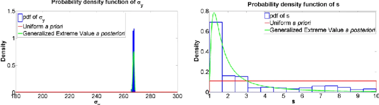
Figure 3: Superposition of the uniform prior distribution, the discrete posterior distribution and the adjusted posterior distribution ( on the left and on the right)
Figure 3 shows the posterior distributions of two parameters. There are non-symmetric distributions that already provide a first level of information about the probabilistic modelling of the variables (Weibull, Lognormal, etc.). The parameter is interesting: it shows that this parameter does not necessarily need to have a wide range of variation. It comes from the model shape and benefits our model because it is very sensitive to this parameter which corresponds to an exponent of Equation (1). Informations about are significant too. The model is very sensitive to this parameter because cannot be chosen far from . We can also consider that is a deterministic variable.
CONCLUSION
The results presented have shown a strong dependence of the model to the material parameters. The parameter is one of the most important. To limit its significant effect on the model response, we shall control its variation range. The updating method has this property and avoids assumptions on the random variables without measurements. The realization of tests will help to enrich the database and to increase confidence in the posterior distributions. This will be possible through crack monitoring or inspections. Indeed, in this article, Bayesian updating is training because we exactly know the experimental tests associated with a Wöhler curve. The SHM let us to know the real time series of stress undergone by the structure. Thus, we will be able to update the material parameters of the model and to predict the remaining lifetime. One condition is to provide a robust and not time-consuming structural model, which is a perspective of this work.
REFERENCES
[1] DNV-RP-C203, Fatigue Design of Offshore Steel Structure, 2011
[2] Dong W., Moan T., Gao Z., “Fatigue reliability analysis of the jacket support structure for offshore wind turbine considering the effect of corrosion and inspection”, Reliability Engineering and System Safety, Elsevier, 2012
[3] Quiniou V., Statistical models of the metocean environment for engineering uses - An operator's needs regarding metocean specifications, September 30, 2013, Brest, France
[4] Lemaitre J., A Course on Damage Mechanics, Dunod, 1996.
[5] Poncelet M., Multiaxialité, hétérogénéité intrinsèques et structurales des essais d’auto-échauffement et de fatigue à grand nombre de cycles, Thèse de doctorat, LMT Cachan, 2007.
[6] Magnusson A. K., Variability of sea state measurements and sensor dependence, September 30, 2013, Brest, France
[7] Lemaitre J., Desmorat R., Engineering Damage Mechanics, Springer, 2004.
[8] De Jesus A. M. P., “A comparison of the fatigue behavior between S355 and S690 steel grades”, Journal
of Construction Steel Research, 2012
[9] Schoefs F., “Sensitivity approach for modelling the environmental loading of marine structures through a matrix response surface”, Reliability Engineering and System Safety, Elsevier, 2008
[10] Dubourg V., Adaptive surrogate models for reliability analysis and reliability-based design optimization, Thèse de doctorat, Université de Blaise Pascal – Clermont II, 2011.
[11] Berveiller M., Le Pape Y., Sudret B., Perrin F., “Bayesian updating of the long-term creep strains in concrete containment vessels using a non-intrusive stochastic finite element method”, ICASP 2007, Application of Statistics and Probability in Civil Engineering, Kanda, Takada and Furuta (eds), 2007, Talor and Francis Group.
[12] Schoefs F., Boukinda M., Guillo C., Rouhan A., “Fatigue of jacket platforms: effect of marine growth modelling”, 24th International Conference on Offshore Mechanics and Arctic Engineering (OMAE), June
12-17, 2005, Halkidiki, Greece
EWSHM 2014 - Nantes, France

![Figure 2: Wohler curve, steel S355J2 by De Jesus [8]](https://thumb-eu.123doks.com/thumbv2/123doknet/8123199.272624/5.892.141.750.708.1091/figure-wohler-curve-steel-s-j-de-jesus.webp)