Infering population history with DIY ABC: a user-friendly
approach to Approximate Bayesian Computation
Jean-Marie Cornueta,b, Filipe Santosb, Mark A. Beaumontc,
Christian P. Robertd, Jean-Michel Marine, David J. Baldinga,
Thomas Guillemaudf and Arnaud Estoupb
April 11, 2008
aDepartment of Epidemiology and Public Health, Imperial College, St Mary’s Campus Norfolk Place, London W2
1PG, U.K.
bCentre de Biologie et de Gestion des Populations,INRA, Campus International de Baillarguet, CS 30016
Montferrier-sur-Lez, 34988 Saint-G´ely-du-Fesc Cedex, France
cSchool of Biological Sciences, Lyle Building, The University of Reading Whiteknights, Reading RG6 6AS, UK
dCEREMADE, Universit´e Paris-Dauphine, Place Delattre de Tassigny,
75775 Paris cedex 16, France
eINRIA Saclay, Projet select, Universit´e Paris-Sud, Laboratoire de Math´ematiques (Bˆat. 425), 91400 Orsay, France
Running head: ABC inference of population history
Corresponding author: Jean-Marie Cornuet
Department of Epidemiology and Public Health, Imperial College St Mary’s Campus, Norfolk Place, London W2 1PG, U.K.
Tel :+44 2075943420
e-mail :[email protected]
Keywords: ABC, Microsatellite, Coalescent, Software, Statistical inference
Abstract: Genetic data obtained on population samples convey information about their evo-lutionary history. Inference methods can extract this information (at least partially) but they re-quire sophisticated statistical techniques that have been made available to the biologist community (through computer programs) only for simple and standard situations typically involving a small number of samples. We propose here a computer program (DIY ABC) for inference based on Approximate Bayesian Computation (ABC), in which scenarios can be customized by the user to fit many complex situations involving any number of populations and samples. Such scenar-ios involve any combination of population divergences, admixtures and stepwise population size changes. DIY ABC can be used to compare competing scenarios, estimate parameters for one or more scenarios, and compute bias and precision measures for a given scenario and known values of parameters (the current version applies to unlinked microsatellite data). This article describes key methods used in the program and provides its main features. The analysis of one simulated and one real data set, both with complex evolutionary scenarios, illustrates the main possibilities of DIY ABC.
Until now, most literature and software about inference in population genetics concern simple
standard evolutionary scenarios: a single population (GRIFFITHS AND TAVARE, 1994; STEPHENS´
ANDDONNELLY, 2000; BEAUMONT, 1999), two populations exchanging genes (HEY ANDNIELSEN,
2004; DEIORIO ANDGRIFFITHS, 2004) or not (HICKERSONet al., 2007) or three populations in
the classic admixture scheme (WANG, 2003; EXCOFFIERet al., 2005). The main exception to our
knowledge is the computer program BAT W IN G (WILSONet al., 2003) which considers a whole
family of scenarios in which an ancestral population splits into as many subpopulations as needed. However, in practice, population geneticists collect and analyse samples that rarely correspond to one of these standard scenarios. If they want to apply methods developed in the literature and for which computer programs are available, they have to select subsets of samples (to fit these standard situations), at the price of lowering the power of the analysis. The other solution is to develop their own software, which requires specific skills or the right collaborators. Rare examples of inference
in non standard scenarios can be found in O’RYANet al. (1998) including 3 populations and two
successive divergences, or ESTOUP et al. (2004) (10 populations that sequentially diverged with
initial bottlenecks and exchanging migrants with neighbouring populations).
Inference in complex evolutionary scenarios can be performed in various ways, but all are based on the genealogical tree of sampled genes and coalescence theory. A first approach used in
pro-grams such as IM (HEY AND NIELSEN, 2004) or BAT W IN G consists in starting from a gene
genealogy compatible with the observed data and exploring the parameter space through MCMC algorithms. In this approach, the tree topology and the branch lengths are parameters in the analysis in the same way as are the scenario parameters. One difficulty with this approach is to be sure that the MCMC has converged, because of the huge dimension of the parameter space. With a complex scenario, the difficulty is increased. Also, although not impossible, it seems quite challenging to write a program that would deal with very different scenarios. A second approach developed by
BEAUMONT (2003) consists in combining MCMC exploration of the scenario parameter space
with an Importance Sampling (IS) based estimation of the likelihood. The strength of this ap-proach is that the low number of parameters ensures a (relatively) fast convergence of the MCMC. Its weakness is that the likelihood is only approximated through IS, sometimes resulting in poor
acceptance rates.
Whith complex scenarios, both previous approaches raise difficulties that mainly stem in the computation/estimation of the likelihood. This prompted a new line of research including the works
of TAVARE´ et al. (1997), WEISS AND VON HAESELER (1998), PRITCHARD et al. (1999) and
MARJORAMet al.(2003) which developed in a new likelihood-free approach termed Approximate
Bayesian Computation (or ABC) by BEAUMONT et al. (2002). In this approach, the likelihood
criterion is replaced by a similarity criterion between simulated and observed data sets, similarity usually measured by a distance between summary statistics computed on both data sets. Among examples of inference in complex scenarios given above, all but one (the simplest) have used this approach, showing that it can indeed solve complex problems.
The ABC approach presents two additional features that can be of interest for experimental
biologist. One characteristic, already noted by EXCOFFIERet al.(2005), is the possibility to assess
the bias and precision of parameter estimates for simulated data sets produced with known values of parameters with y little extra computational cost. To get the same important information with likelihood-based methods would require a huge amount of additional computations whereas, with ABC, the largest proportion of computations used for estimating parameters can be recycled in a bias/precision analysis. The second feature is the simple way by which the posterior probability
of different scenarios applied to the same data set can be estimated (E.G. MILLER et al., 2005;
PASCUALet al., 2007; FAGUNDESet al., 2007).
However, in its current state, the ABC approach remains inaccessible to most biologists because there is not yet a simple software solution. In order to fill this gap, we developed the program DIY ABC that performs ABC analyses on complex scenarios. By complex scenarios, we mean scenarios which include any number of populations and samples (samples possibly taken at differ-ent times), with populations related by divergence and/or admixture evdiffer-ents and possibly experienc-ing changes of population size. The current version is restricted to unlinked microsatellite data. In this article, we describe the rationale for some methods involved in the program. Then we give the main features of DIY ABC and we provide two complete example analyses performed with this program to illustrate its possibilities.
KEY METHODS INVOLVED IN DIY ABC
Inference about the posterior distribution of parameters in an ABC analysis is usually performed in three steps (Figure 1). The first one is a simulation step in which a very large table (the refer-ence table) is produced and recorded. Each row corresponds to a simulated data set and contains the parameter values used to simulate the data set and summary statistics computed on the simu-lated data set. Parameter values are drawn from prior distributions. Using these parameter values, genetic data are simulated as explained in the next section. The summary statistics correspond to those traditionnally used by population geneticists to characterize the genetic diversity within and among samples (e.g. number of alleles, genic diversity and genetic distances). The idea is to extract maximum genetic information from the data, admitting that exhaustivity or sufficiency are generally out of reach. The simulation step is generally the most time-consuming step since the
number of simulated data sets generally lies between 105 and 107. The second step is a rejection
step. Euclidian distances between each simulated and the observed data set in the space of sum-mary statistics are computed and only the simulated data sets closest to the observed data set are retained. The parameter values used to simulate these selected data sets provide a sample of
param-eter values approximately distributed according to their own posterior distribution. BEAUMONT et
al. (2002) have shown that a local linear regression (third step = estimation step) provides a better
approximation of the posterior distribution.
This synoptic of ABC is now well established and we now concentrate on more specific issues that are implemented in DIY ABC.
Simulating genetic data in complex scenarios
Thanks to coalescence theory, it has become easy to simulate data sets by a two steps procedure. The first step consists of building a genealogical tree of sampled genes according to rather simple rules provided by coalescence theory (see below). The second step consists of attributing allelic states to all the nodes of the genealogy, starting from the common ancestor and simulating muta-tions according to the mutation model of the genetic markers. In a complex scenario, only the first
step needs special attention and we will concentrate on it now.
In a single isolated population of constant effective size, the genealogical tree of a sample of genes is simulated backward in time: starting from the time of sampling, the gene lineages are merged (coalesced) at times that are drawn from an exponential distribution with rate j(j − 1)/4N , when there are j distinct lineages and the (diploid) effective population size is N . The genealogical tree is completed when there remains a single lineage.
Consider now two isolated populations (effective population sizes N1 and N2respectively) that
diverged td generations before their common sampling time. Since the two populations do not
exchange genes, lineages within each population will coalesce independently. Coalescence simula-tion will stop either when there remains a single lineage or when the simulated time is beyond the divergence (looking back in time). In the latter case, the coalescence event is simply discarded. De-pending on whether the last (not discarded) coalescence or the divergence time comes first (looking backward in time), there will remain one or more gene lineages in each population at generation
td. In any case, the remaining lineages of both populations are simply pooled and will coalesce
in the ancestral population. Because of the memoryless property of the exponential distribution, the time to the first coalescence in the ancestral population is independent of the times of the last coalescence in each daughter population and can be simulated as in the single isolated population above. Again, the genealogical tree is completed when there remains a single lineage in the ances-tral population. Note that the two populations need not be sampled at the same generation since this has no bearing on the simulation process other than giving the two populations different number of generations for simulating coalescences before divergence.
Consider now the classic admixture scenario with one admixed and two parental populations,
as in Figure 1 in EXCOFFIER et al. (2005). Simulating the complete genealogical tree can be
achieved with the following steps: i) coalesce gene lineages in each population independently until reaching admixture time, ii) distribute remaining lineages of the admixed population among the two parental populations, each with a Bernoulli draw with probability equal to the admixture rate, iii) coalesce gene lineages in the two parental populations until reaching their divergence time, iv) pool the remaining gene lineages of the two parental populations and place them into the ancestral
population, and v) coalesce gene lineages in the ancestral population.
We first note the modular form of this algorithm which involves only three modules:
1. a module that performs coalescences in an isolated constant size population between two given times/generations,
2. a module that pools gene lineages from two populations (for divergence),
3. a module that splits gene lineages from the admixed population between two parental popula-tions (for admixture).
We also note that discrete changes of population size can be simulated with the first module just varying the effective population size parameter value when the time of change is reached. It might also be extended to include continuous (linear or exponential) size variations.
We have introduced a fourth module that proves useful in many instances. It performs the (simple) task of adding a gene sample to a population at a given generation. The interest of this module is to allow for multiple samples of the same population taken at different generations. By combining the aforementionned four modules, it is possible to simulate genetic data involving any number of populations according to a scenario that can include divergence, admixture events as well as population size variations. In addition, populations can be sampled more than once at different times. Compared to our previous definition of complex scenarios, the only restriction so far concerns the absence of migrations among populations. If migrations have to be taken into account, coalescences in two (or more) populations exchanging migrants are no longer independent and should be treated in the same module. Such a module would require to consider simultaneously two kind of events, coalescences of lineages within population and migrations of gene lineages from one population to another. In the current stage of DIY ABC, this has not yet been achieved.
Two ways of simulating colescence events
Simulating coalescences can be performed in two ways. The most traditional way is based on the usually fulfilled assumption that the effective population size is large enough so that the probability
of coalescence is small and hence that the probability that two coalescences occur at the same generation is low enough so that it can be neglected. Time is then considered as a continuous
variable in computations (see NORDBORG (2007) for a detailed explanation). The corresponding
algorithm, called here the continuous time (CT) algorithm, consists in drawing first times between
two successive coalescence events (these times are exponentially distributed with rates equal to (k2)
when there are k remaining lineages) and then drawing 2 lineages at random at each coalescence event).
However, in practice, population size can be so small (e.g. during a bottleneck) that multiple coalescences at the same generation become common, including with the same parental gene (pro-ducing multifurcating trees). Simulating gene genealogies with multiple coalescences is possible,
(E.G. LAVAL AND EXCOFFIER, 2004). In effect, lineages are reconstructed one generation at a
time: lineages existing at generation g are given a random number drawn in U [1, 2N ] and lin-eages with the same number coalesce at generation g+1. This second algorithm is termed here the generation by generation (GbG) algorithm. It corresponds exactly to the Wright-Fisher model definition.
The CT algorithm is much faster in most cases and is generally prefered in many softwares, but in some circunstances, the approximation becomes inacceptable. The solution taken in DIY ABC is to swap between the two methods according to a criterion based on the effective population size, the time during which the effective size keeps its value, and the number of lineages at the start of the module. The criterion is such that the generation per generation (GbG) algorithm is taken whenever it is faster (this can occur when the effective size is very small) or when the continuous time (CT) algorithm produces on average a number of lineages at the end of the module that is more than 5% larger than that obtained through the GbG algorithm.
A specific comparison study has been performed to establish this criterion. For different time
periods (counted in generations), effective population sizes (Ne) and number of entering lineages
(nel), coalescences have been simulated according to each algorithm 10,000 times and the average
number of remaining lineages at the end of the period have been recorded as well as the average computation duration of each algorithm. Three types of output were distinguished:
1. the CT algorithms produced an average number of coalescences that differred from that of GbG by at least 5%;
2. the CT algorithm produced an average number of coalescences within 5% of that produced by the GbG, but the GbG was faster;
3. the CT algorithm produced an average number of coalescences within 5% of that produced by the GbG, and it was faster.
Only in the situation (3) is the CT advantageous over the GbG. Figure 2 shows that the boundary separating situation (3) from the other two is quasi-linear with zero intercept and a slope that varies with the duration (g counted in generations) of the coalescence module. We found that a piecewise approximation of the slope as a function of g provided a good fit of the limit of the area in which the CT algorithm could advantageously replace the GbG algorithm. DIY ABC hence uses the following decision rules:
if (1 < g ≤ 30) do CT if nel/Ne< 0.0031g2− 0.053g + 0.7197 else do GbG
if (30 < g ≤ 100) do CT if nel/Ne< 0.033g + 1.7 else do GbG
if (100 < g) do CT if nel/Ne < 5 else do GbG
Comparing scenarios
Using ABC to compare different scenarios and infer their posterior probability has been performed in two ways in the literature. Starting with a reference table containing parameters and summary statistics obtained with the different scenarios to be compared (or pooling reference tables, each obtained with a given scenario), data sets are ordered by increasing distance to the observed data set. A first way (termed hereafter the direct approach) is to take as an estimate of the posterior
probability of a scenario the proportion of data sets obtained with this scenario in the nδ closest
data sets (MILLER et al., 2005; PASCUAL et al., 2007). The value of nδ is arbitrary and unless
the results are quite clear cut, the estimated posterior probability may vary with nδ.
Following the same rationale that introduced the local linear regression in the estimation of
et al., 2007) suggested to perform a weighted polychotomous logistic regression to estimate the posterior probability of scenarios (termed hereafter the logistic approach). In the estimation of parameters, a linear regression is performed with dependent variable the parameter and predictors the differences between the observed and simulated statistics. This linear regression is local at the point (in the predictor space) corresponding to the observed data set, using an Epanechnikov kernel based on the distance between observed and simulated summary statistics . Parameters values are then replaced by their estimates at that point in the regression. Since that point is the origin of the predictor space (null coordinates), the estimate is the sum of the constant term of the regression (intercept) and the residual in the regression.
Keeping the differences between observed and simulated statistics as the predictor variables in the regression, we consider now the posterior probability of scenarios as the dependent variable. Because of the nature of the ”parameter”, an indicator of the scenario number, a logit link function is applied to the regression. The local aspect of the regression is obtained by taking the same Epanechnikov weights as in the linear adjustment of parameter values as described in BEAUMONT
et al.(2002). Confidence intervals for the posterior probabilities of scenarios are computed through
the limiting distribution of the maximum likelihood estimators. See Appendix 1 for more details.
Quantifying confidence in parameter estimations on simulated test data sets
In order to be confident in estimates, these should be unbiased and precise enough. In order to measure bias and precision, we need to simulate data sets (i.e. test data sets) with known values of parameters and compare estimates with their true values. In the ABC estimation procedure, the most time-consuming task is to produce a large enough reference table. However, when such a reference table has been produced, e.g. for the analysis of a real data set, it can also be used to quantify bias and precision on test data sets as well.
Measuring bias is straightforward, but precision can be assessed with different measures. In DIY ABC, the latter include the relative square root of the mean square error, the relative square root of the mean integrated square error, the relative mean absolute deviation, the 50 and 95%
coverages and the factor 2. See Appendix 2 for precise definitions of these indices.
DIY ABC: A COMPUTER PROGRAM FOR POPULATION BIOLOGISTS
Main features
DIY ABC is a program that performs ABC inference on population genetics data. In its current state, the data are genotypes at microsatellite loci of samples of diploid individuals representative of populations. The inference bears on the evolutionary history of the sampled populations by quantifying the relative support of data to possible scenarios and by estimating posterior densities of associated parameters. DIY ABC is a program written in Delphi running under a 32-bit Windows operating system (e.g. Windows XP) and it has a user-friendly graphical interface.
The program accepts complex evolutionary scenarios including any number of populations and samples. Scenarios can include unsampled as well as multi-sampled (at different times) popula-tions. Missing data are allowed. Scenarios can include any number of the following timed events: stepwise change of effective population size, population divergence and admixture. The main re-striction regarding scenario complexity is the absence of migrations between populations after they have diverged.
Since the program has been written for microsatellite data, it proposes two popular mutation models, namely the stepwise mutation model and the generalized stepwise mutation model
(ES-TOUPet al., 2002). In addition, it includes single nucleotide mutations to simulate uneven
inser-tion/deletion events commonly observed in real microsatellite data sets ( PASCUAL et el., 2007;
see also example in section 2.2.2). Note that the same mutation model has to be applied to all microsatellite loci, but these may have different values of mutation parameters except for the prob-ability of a single nucleotide mutation which is common to all loci.
The historico-demographic parameters of the studied evolutionary scenarios may be of three types: effective sizes, times of events (in generations) and admixture rates. Marker parameters are mutation rates and the coefficient of the geometric distribution (under the GSM only). The program
effective population size, t the time of an event and µ the mean mutation rate. Prior distributions are defined for original parameters and those for composite parameters are obtained via an assumption of independence of their component prior densities. Priors for historico-demographic parameters can be chosen among four common distributions: Uniform, Log-uniform, Normal and Log-normal. Users can set minimum and maximum (for all distributions), mean and standard deviation (for Normal and Log-normal) and a step value that can be used to round values. In addition, priors can be modified by setting binary conditions on pairs of parameters of the same category (two effectives sizes or two times of event). These binary conditions are >, <, ≥ and ≤. This is especially useful to control the relative times of events when these are parameters of the scenario. For priors of mutation parameters, only the Uniform and the Gamma distribution are considered, the latter being defined by the mean and the shape. The choice of the mean is meant to facilitate the implementation of a hierarchical scheme, with a mean mutation rate or coefficient P drawn from a given prior and individual loci parameter values drawn from a gamma distribution around the mean.
Available summary statistics are usual population genetic statistics averaged over loci: e.g. mean
number of alleles, mean genic diversity, FST, (δµ)2or admixture rates.
Regarding ABC computations, the program can i) create a reference table or append values to an existing table, ii) compute the posterior probability of different scenarios on the same data set, iii) estimate the posterior distributions of original and/or composite parameters for one or more scenarios and iv) compute bias and precision for a given scenario and given values of parameters . Finally, the program can be used simply to simulate data sets in a format compatible with the
program Genepop (RAYMOND ANDROUSSET, 1995).
Two examples of analysis with DIY ABC
Illustration on a simulated data set: In order to illustrate the capabilities of DIY ABC, we take first an example based on a simulated data set. To produce this data set, we used the corresponding option of the program. The data set has been simulated according to a complex scenario including
three splits and two admixture events1 (scenario 1 in Figure 3). The scenario also includes six populations: two of them have been sampled at time 0, the third one at time 2 and the fourth one at time 4, the last two have not been sampled. Each population sample includes 30 diploid individuals and data are simulated at 10 microsatellite loci. Each locus has a possible range of 40 contiguous allelic states and is assumed to follow the GSM with µ drawn from a Gamma(mean=0.0005 and shape=2) and P drawn from a Gamma(mean=0.22 and shape=2). Our ABC analysis will address the following questions:
1. Suppose that we are not sure that the scenario having produced our example data set does include a double admixture and that we want to challenge this double admixture scenario with two simpler scenarios, one with a single admixture (scenario 2 in Figure 3) and the other with no admixture at all (scenario 3 in Figure 3). What is the posterior probability of these three scenarios, giving them identical prior probabilities ?
2. What are the posterior distributions of parameters, given that the right scenario is known ? 3. What confidence can we have into the parameter estimation ?
We need first to build up the reference table. Using different screens of DIY ABC, i) we code the three scenarios and define the prior distribution of parameters (Figure S1 provided in Supple-mentary data), ii) we select the GSM and define prior distribution for the mutation parameters (Figure S2), iii) we set the motif size and the allele range of each locus (Figure S3) and iv) we select a set of summary statistics (Figure S4). Eventually, we start running simulations and after some hours (on a laptop), we get a reference table with 6 million simulated data sets (i.e. 2 million per scenario).
To answer the first question, we run the option ”compute posterior probabilities of scenario”,
taking the nδ=60,000 (1%) simulated data sets closest to the pseudo-observed data set for the
lo-gistic regression and nδ=600 (0.01%) for the direct approach. The answer appears in two graphs
1This scenario is not purely theoretical as it could be applied for instance to European populations of honeybees in which the Italian populations
(Apis mellifera ligustica result from an ancient admixture between two evolutionary branches (FRANCKet al., 2000) that would correspond here
to population samples 1 and 4. Furthermore, in the last 50 years, Italian bees have been widely exported in other countries and sample 2 could well correspond to a population of a parental branch that has been recently introgressed by Italian queens. This example also stresses the ability of DIY ABC to distinguish two events that are confounded in the usual admixture scheme: the admixture event itself and the time at which the real parental populations in the admixture diverged from the population taken as ”parental”.
(Figure 4). Clearly both approaches are congruent and show that scenario 1 is significantly better supported by data than any other scenarios.
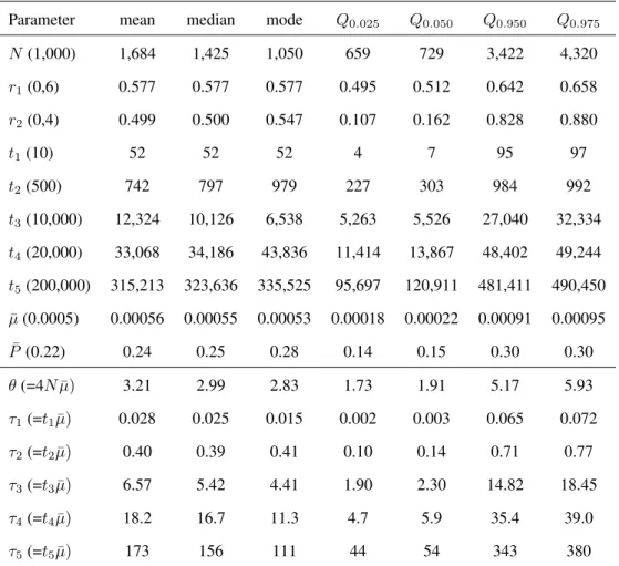
To answer the second question, we run the option ”estimate parameters” choosing the first sce-nario. Here again, we take the 20,000 (1%) closest simulated data sets. Output include graphs providing the prior and posterior distributions of the corresponding parameter, as well as mean, median, modes and four quantiles (Figure S5). Under each graph on the DIY ABC screen are given the mean, median and mode as well as four quantiles (0.025, 0.05, 0.95 and 0.975) of the posterior distribution (Table 1). Since we know the true values, we can remark that some parame-ters are rather well estimated with peaked posteriors such as the common effective population size
and the admixture rate r1, whilst data are not very informative for other parameters.
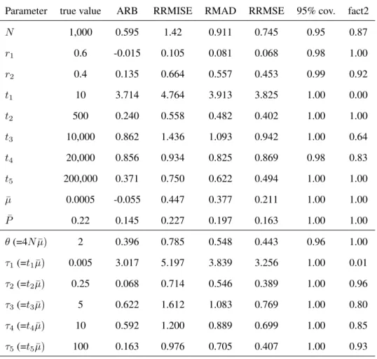
To evaluate quantitatively the amount of confidence that can be put into the parameter estima-tions, we run the option ”compute bias and precision” on 100 test data sets with known parameter values, using the same proportion (1%) of closest simulated data sets as above. This requires a few hours at the end of which we have a complete table (see extract in Table 2) showing relative biases and dispersion measures. It is clear that several parameters are biased and/or dispersed, the worst
case being that of parameter t1. The bias is undoubtedly related to the lack of information in the
data, so that point estimates are drawn towards the mean values of prior distributions.
Illustration on a real data set: As a second example to illustrate analysis with DIY ABC, we have chosen a real microsatellite data set obtained from several Pacific island populations of
the bird Zosterops lateralis lateralis, commonly named silvereye (ESTOUP AND CLEGG, 2003).
During the 19th and 20th century, this bird colonised Southwest Pacific islands from Tasmania. The importance of single founder events in the microevolution of this species has been questioned
in a study based on a six microsatellite loci data set (CLEGG et al, 2002), where single founder
events were found to have relatively low impact on shaping the neutral genetic variation of at least some island populations of silvereyes.
Our analysis with DIY ABC differs by at least four aspects from the initial ABC analysis
are treated here in the same analysis whereas, for tractability reasons, the populations have been treated independently by pair with Tasmania as source population in each pair and different
num-ber of founder events by ESTOUP AND CLEGG (2003). Second, because parameter estimation in
DIY ABC is based on the local linear regression method of BEAUMONT et al. (2002), we could
use a much larger number of statistics (see below), and hence better summarize information from
the data, than in the initial ABC treatment that was based on the algorithm of PRITCHARD et al.
(1999). Third, we have chosen non informative flat priors for all demographic parameters. Fourth, because DIY ABC is able to treat samples collected at different times, we did not have to pool samples collected at different years from the same island and average sample year collection over islands. We hence end up with a colonization scenario involving five populations and seven sam-ples, two samples having been collected at different times in two different islands (Figure 5). The sequence and dates of colonisation by silvereyes to New Zealand (South and North Island) and outlying islands (Chatham and Norfolk islands) have been historically documented. This allows fixing the times for the putative population size fluctuation events in the coalescent gene trees, and hence to limit the number of parameters in our sequential colonization with founder event scenario. Our scenario was specified by six variable demographic parameters: the stable effective population
size (NS) which was assumed to be the same in all islands, potentially different effective number
of founding individuals in Norfolk island, Chatham island and the South and North island of New
Zealand (NF 1, NF 2, NF 3and NF 4, respectively), and the duration of the bottleneck associated with
the foundation of new populations (DB), which was assumed to be the same for all colonization
events. As in ESTOUP ANDCLEGG(2003), we also assumed that all populations evolved as totally
isolated demes after the date of colonisation.
We chose uniform prior distributions bounded between 300 and 30,000 for NS, between 2 and
500 for all NF i and between 1 and 5 for DB. It is worth noting that the durations of the
bottle-neck, the effective numbers of individuals during the bottlenecks and the stable effective popula-tion size are barely individually identifiable in the likelihood. Therefore, we also computed for each colonized population a combined parameter called the bottleneck severity index computed
and their posterior distributions were computed from the original parameters values obtained after
the regression step using the R package (IHAKA AND GENTLEMAN, 1996). Prior information
regarding the mutation rate and model for dinucleotide repeats was the same as in the previous example, except that observed allele size differences indicate a larger possible range of contiguous allelic states (set to 70 for all loci). Regarding uneven insertion/deletion events that could be sus-pected for most loci from observed allele sizes, we used a Gamma prior distribution with mean=
2.5 × 10⁻⁸ and shape=2 for drawing single locus insertion-deletion mutation rates (PASCUAL et
al., 2007). Genetic variation within and between the seven population samples was summarized
with the same summary statistics as in MILLER et al. (2005) and PASCUAL et al. (2007), i.e.
the mean number of alleles (A), the mean genic diversity (H ; NEI, 1987), the mean ratio of the
number of alleles over the range of allelic sizes per population expressed in base pairs (M ; GARZA
ANDWILLIAMSON, 2001), FST between pairs of population samples (WEIR ANDCOCKERHAM,
1984), and the mean classification index for individuals collected in the population sample i and assigned to the population j (also called mean individual assignment likelihood; cf. formula 9 in Rannala and Mountain 1997). We hence had a total of 84 summary statistics. We produced a reference table with 1 million simulated data sets and estimate parameter posterior distributions taking the 10,000 (1%) simulated data sets closest to the observed data set for the local linear re-gression, after applying a logit transformation to parameter values. Similar results were obtained when taking the 2,000 to 20,000 closest simulated data sets and when using a log or log − tangent
transformation of parameters as proposed in ESTOUPet al. (2004) and HAMILTONet al. (2005)
(options available in DIY ABC).
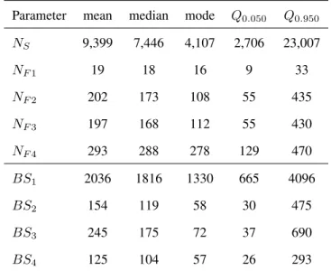
Results for the main demographic parameters are presented in Table 3. They indicate the colo-nization by a small number of founders and/or a slow demographic recovery after foundation for
Norfolk island only (median NF 1value of 18 individuals). Other island populations appear to have
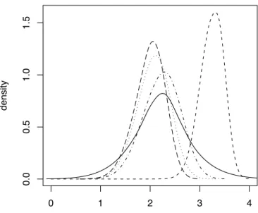
been founded by silvereye flocks of larger size and/or have recovered quickly after foundation. In agreement with this, the bottleneck severity was more than one order of magnitude larger for the population from Norfolk than for other island populations (Figure 6). These results are in the same
Discrepancies in parameter estimation are observed however (e.g. larger NS values and more
pre-cise inferences for NF 2, NF 3 and NF 4 in the present treatment). Such discrepancies are expected
due to the differences in the methodological design underlined above. With the possibility of treat-ing all population samples together, DIY ABC allows a more elaborate and satisfactory treatment
compared to previous analyses (ESTOUP ANDCLEGG, 2003; MILLERet al., 2005).
Conclusion
So far, the ABC approach remained inaccessible to most biologists because of the complex com-putations involved. With DIY ABC, non specialists can now perform ABC-based inference on various and complex population evolutionary scenarios, without reducing them to simple standard situations and hence making a better use of their data. In addition, this programs also allows them to compare competing scenarios and quantify their relative support by the data. Eventually, it pro-vides a way to evaluate the amount of confidence that can be put into the various estimations. The main limitations of the current version of DIY ABC are the assumed absence of migration among populations after they have diverged and the mutation models which mostly refer to microsatellite loci. Next developments will aim at progressively remove these limitations.
Acknowledgements
The development of DIY ABC has been supported by a grant from the French Research National Agency (project M ISGEP OP ) and a grant from the European Union awarded to JM Cornuet as an EIF Marie-Curie Fellowship (project StatInf P opGen) that allowed him to spend two years in DJ Balding’s Epidemiology and Public Health department at Imperial College (London, UK) where he wrote the major part of this program.
We are most grateful to Sonia Clegg for authorizing the use of Silvereye microsatellite data in our second example.
References
BEAUMONT, M.A., 1999. Detecting population expansion and decline using microsatellites. Ge-netics, 153, 2013-2029.
BEAUMONT, M.A., 2003. Estimation of population growth or decline in genetically monitored populations, Genetics, 164, 1139-1160.
BEAUMONT, M.A., 2008. Joint determination of topology, divergence time, and immigration in population trees. In Simulation, Genetics, and Human Prehistory, eds. S. Matsumura, P. Forster, C. Renfrew. McDonald Institute Press, University of Cambridge (in press).
BEAUMONT, M. A., W. ZHANG ANDD. J. BALDING, 2002. Approximate Bayesian Computation
in Population Genetics. Genetics 162, 2025-2035.
BERTORELLE, G.ANDL. EXCOFFIER, 1998. Inferring admixture proportion from molecular data.
Mol. Biol. Evol.15, 1298-1311.
CHOISY, M., P. FRANCK AND J.M. CORNUET, 2004. Estimating admixture proportions with
microsatellites: comparison of methods based on simulated data. Mol. Ecol. 13, 955-968.
CHAKRABORTYR AND L JIN, 1993. A unified approach to study hypervariable polymorphisms:
statistical considerations of determining relatedness and population distances. EXS. 67, 153175.
CLEGGS.M., S.M. DEGNAN, J. KIKKAWA, D. MORITZ, A. ESTOUP ANDI.P.F. OWENS, 2002.
Genetic consequences of sequential founder events by an island colonising bird. Proc. Nat. Acad.
Sc.99, 8127-8132.
DE IORIO, M. AND R.C. GRIFFITHS, 2004. Importance sampling on coalescence histories. ii:
subdivided population models. Advanc. Appl. Probab. 36, 434-454.
ESTOUP, A., I. J. WILSON, C. SULLIVAN, J. M. CORNUET AND C. MORITZ, 2001. Inferring
population history from microsatellite et enzyme data in serially introduced cane toads, Bufo marinus. Genetics, 159, 1671-1687.
ESTOUP, A., P. JARNE AND J.M. CORNUET, 2002. Homoplasy and mutation model at microsatel-lite loci and their consequences for population genetics analysis. Mol. Ecol., 11, 1591-1604.
ESTOUP, A.ANDS. M. CLEGG, 2003. Bayesian inferences on the recent islet colonization history
by the bird Zosterops lateralis lateralis. Mol. Ecol. 12: 657-674.
ESTOUP, A., M.A. BEAUMONT, F. SENNEDOT, C. MORITZ ANDJ.M. CORNUET, 2004. Genetic
analysis of complex demographic scenarios: spatially expanding populations of the cane toad, Bufo marinus. Evolution,58, 2021-2036.
FAGUNDES, N.J.R., N. RAY, M.A. BEAUMONT, S. NEUENSCHWANDER, F. SALZANO, S.L.
BONATTO ANDL. EXCOFFIER, 2007. Statistical evaluation of alternative models of human
evo-lution. Proc. Natl. Acad. Sc., 104 : 17614-17619.
FRANCK, P., L. GARNERY, G. CELEBRANO, M. SOLIGNAC ANDJ.M. CORNUET, 2000. Hybrid
origins of honeybees from Italy (Apis mellifera ligustica) and Sicily (A. m. sicula). Mol. Ecol., 9, 907-92.
EXCOFFIER, L., A. ESTOUP ANDJ.M. CORNUET, 2005. Bayesian analysis of an admixture model
with mutations and arbitrarily linked markers. Genetics 169, 1727-1738.
FU, Y.X.ANDR. CHAKRABORTY, 1998. Simultaneous estimation of all the parameters of a
step-wise mutation model. Genetics, 150, 487-497.
GARZA J.C. AND E. WILLIAMSON, 2001. Detection of reduction in population size using data
from microsatellite DNA. Mol. Ecol. 10,305-318.
GOLDSTEIN D.B., A.R. LINARES, L.L. CAVALLI-SFORZA AND M.W. FELDMAN, 1995. An
evaluation of genetic distances for use with microsatellite loci. Genetics 139, 463471.
GRIFFITHS, R.C. AND S. TAVARE, 1994. Simulating probability distributions in the coalescent.´
Theor. Pop. Biol.46, 131-159.
social regulation of immigration in patrilocal populations than in matrilocal populations. Proc. Natl. Acad. Sci. USA, 102, 7476-7480.
HEY, J. AND R. NIELSEN, 2004. Multilocus methods for estimating population sizes, migration
rates and divergence time, with applications to the divergence of Drosophila pseudoobscura and D. persimilis. Genetics, 167, 747-760.
HICKERSON, M.J., E. STAHL ANDN. TAKEBAYASHI, 2007. msBayes: Pipeline for testing
com-parative phylogeographic histories using hierarchical approximate Bayesian computation. BMC Bioinformatics, 8, 268-274.
IHAKAR. ANDR. GENTLEMAN, 1996. R: a language for data analysis and graphics. J. Comput.
Graph. Stat., 5, 299-314
LAVAL, G., AND L. EXCOFFIER, 2004. SIMCOAL 2.0: a program to simulate genomic diversity
over large recombining regions in a subdivided population with a complex history. Bioinformat-ics, 20: 2485-2487.
MARJORAM, P., J. MOLITOR, V. PLAGNOL AND S. TAVARE, 2003. Markov chain Monte Carlo´
without likelihood. Proc. Natl. Acad. Sc., 100, 15324-15328.
MILLER N, A. ESTOUP, S. TOEPFER, D BOURGUET, L. LAPCHIN, S. DERRIDJ, K.S. KIM, P
REYNAUD, F. FURLAN AND T. GUILLEMAUD, 2005. Multiple Transatlantic Introductions of
the Western Corn Rootworm. Science, 310, p. 992
NEIM., 1987. Molecular Evolutionary Genetics. Columbia University Press, New York, 512 pp.
NORDBORG, M., 2007. Coalescent theory p843-877 in Handbook of Statistical Genetics Ed. by D.J. Balding, M. Bishop and C. Cannings, 3rd ed., Wiley & Sons, Chichester, U.K.
OHTA, T. AND M. KIMURA, 1973. A model of mutation appropriate to estimate the number of
electrophoretically detectable alleles in a finite population.
HARLEY, 1998. Genetics of fragmented populations of African buffalo (Syncerus caffer) in South Africa. Animal Conservation, 1, 85-94.
PASCUAL, M., M.P. CHAPUIS, F. MESTRES, J. BALANYA, R.B. HUEY, G.W. GILCHRIST,´
L. SERRA AND A. ESTOUP, 2007. Introduction history of Drosophila subobscura in the New
World: a microsatellite based survey using ABC methods. Mol. Ecol., 16, 3069-3083.
PRITCHARD, J., M. SEIELSTAD, A. PEREZ-LEZAUN AND M. FELDMAN, 1999. Population
growth of human Y chromosomes: a study of Y chromosome microsatellites. Mol. Biol. Evol. 16, 1791-1798.
RANNALA, B., AND J. L. MOUNTAIN, 1997. Detecting immigration by using multilocus
geno-types. Pro. Nat. Acad. Sci. USA 94, 9197-9201.
RAYMOND M.,AND F. ROUSSET, 1995. Genepop (version 1.2), population genetics software for
exact tests and ecumenicism. J. Hered., 86, 248-249
STEPHENS, M. AND P. DONNELLY, 2000. Inference in molecular population genetics (with
dis-cussion). J. R. Stat. Soc. B 62, 605-655.
TAVARE´ S., D.J. BALDING, R.C. GRIFFITHS AND P. DONNELLY, 1997. Inferring coalescence
times from DNA sequences. Genetics, 145, 505-518.
WANG, J., 2003. Maximum-likelihood estimation of admixture proportions from genetic data. Genetics, 164, 747-765.
WEIR B.S.AND C.C. COCKERHAM, 1984. Estimating F-statistics for the analysis of population
structure. Evolution 38: 1358-1370.
WEIS, G. AND A. VON HAESELER, 1998. Inference of population history using a likelihood
ap-proach. Genetics, 149, 1539-1546.
WILSON, I.J., M.E. WEALE AND D.J. BALDING, 2003. Inferences from DNA data: population
histories,evolutionary processes, and forensic match probabilities. J. R. Stat. Soc. A 166, 155-187.
Figure legends
Figure 1 : The three steps of an ABC analysis. The two boxes with a double line correspond to the case where there are more than one scenario.
Figure 2 : Which algorithm for the coalescence module ? Graphs indicate in light grey the area of the plane for which the generation by generation (GbG) algorithm is faster than the con-tinuous time (CT) algorithm, in middle grey the area for which the CT algorithm produces significantly (5%) less coalescences than the GbG algorithm and in dark grey the area for which the CT algorithm produces the same number of coalescences than the GbG algorithm (with tolerance=5%) and is faster. Limits between areas are almost linear. The black line
(intercept=0) has a slope taken as 0.0031g2− 0.053g + 0.7197 for g ≤ 30, 0.033g + 1.7 for
30 < g ≤ 100 and 5 when 100 < g, g being the duration of the coalescence module in number of generations.
Figure 3 : First example: the three evolutionary scenarios. The data set used as an example has been simulated according to scenario 1 (left). The parameter values were the following: all populations had an effective (diploid) size of 1,000, the times of successive events (backward in time) were t1=10, t2=500, t3=10,000, t4=20,000 and t5=200,000, the two admixture rates
were r1=0.6 and r2=0.4. Scenario 1 includes 6 populations, the four that have been sampled
and two left parental populations in the admixture events. Scenario 2 and 3 include 5 and 4 populations respectively. Time is not at scale. Samples 3 and 4 have been collected 2 and 4 generations earlier than the first two samples, hence their slightly upward locations on the graphs.
Figure 4 : First example: posterior probability of scenarios. The x-axis correspond to the different
nδ values used in the computations and the y-axis gives the posterior probability of the three
scenarios through the direct (left) and the logistic (right) approaches as output by DIY ABC. In both graphs, the upper curve corresponds to scenario 1.
set. On the left is the scenario codification for DIY ABC and on the right is the correspond-ing graphic representation produced by the program. Note the keyword varNe to inform of a change in effective size of populations. This keyword is followed by the population num-ber and the new population size. In 1830, Z. l. lateralis colonised the South Island of New Zealand (Pop2) from Tasmania (Pop1). In the following years, the population began expand-ing and dispersexpand-ing, and reached the North Island by 1856 (Pop3). Chatham Island (Pop4) was colonised in 1856 from the South Island, and Norfolk Island (Pop5) was colonised in 1904 from the North Island (historical information reviewed in Estoup and Clegg 2003). Sample collection times are 1997 for Tasmania (Sa1), South and North island of New Zealand (Sa2 and Sa3, respectively), Chatham island (Sa4) and Norfolk island (Sa5), 1994 for the second sample from Norfolk (Sa6), and 1992 for the second sample from the North island of New Zealand (Sa7). Splitting events and sampling dates in years were translated in number of generations since the most recent sampling date by assuming a generation time of three years (Estoup and Clegg 2003). We hence fixed t1, t2, t3 and t4 to 31, 47, 47 and 56 generations, respectively.
Figure 6 : Second example: posterior distributions of the bottleneck severity for the successive invasions of four Pacific islands by Zosterops lateralis lateralis. The four discontinuous lines with small dashes, dots, dash-dots and long dashes correspond to Norfolk, Chatham, North Island and South Island of New Zealand, respectively. The continuous line corresponds to the prior distribution, which is identical for each island. This graph has been made with the R
locfitfunction, using an option of DIY ABC which allows to save the sample of the parameter
Table 1: First example: statistics of the posterior distribution of parameters under scenario 1
Parameter mean median mode Q0.025 Q0.050 Q0.950 Q0.975
N (1,000) 1,684 1,425 1,050 659 729 3,422 4,320 r1(0,6) 0.577 0.577 0.577 0.495 0.512 0.642 0.658 r2(0,4) 0.499 0.500 0.547 0.107 0.162 0.828 0.880 t1(10) 52 52 52 4 7 95 97 t2(500) 742 797 979 227 303 984 992 t3(10,000) 12,324 10,126 6,538 5,263 5,526 27,040 32,334 t4(20,000) 33,068 34,186 43,836 11,414 13,867 48,402 49,244 t5(200,000) 315,213 323,636 335,525 95,697 120,911 481,411 490,450 ¯ µ (0.0005) 0.00056 0.00055 0.00053 0.00018 0.00022 0.00091 0.00095 ¯ P (0.22) 0.24 0.25 0.28 0.14 0.15 0.30 0.30 θ (=4N ¯µ) 3.21 2.99 2.83 1.73 1.91 5.17 5.93 τ1(=t1µ)¯ 0.028 0.025 0.015 0.002 0.003 0.065 0.072 τ2(=t2µ)¯ 0.40 0.39 0.41 0.10 0.14 0.71 0.77 τ3(=t3µ)¯ 6.57 5.42 4.41 1.90 2.30 14.82 18.45 τ4(=t4µ)¯ 18.2 16.7 11.3 4.7 5.9 35.4 39.0 τ5(=t5µ)¯ 173 156 111 44 54 343 380
Mean, median, mode and quantiles of the posterior distribution sample for original and compos-ite parameters of the simulated data set. True values of original parameters (used to simulate the data set) are given between parentheses in the first column.
Table 2: First example: bias and precision of parameter estimation under scenario 1
Parameter true value ARB RRMISE RMAD RRMSE 95% cov. fact2
N 1,000 0.595 1.42 0.911 0.745 0.95 0.87 r1 0.6 -0.015 0.105 0.081 0.068 0.98 1.00 r2 0.4 0.135 0.664 0.557 0.453 0.99 0.92 t1 10 3.714 4.764 3.913 3.825 1.00 0.00 t2 500 0.240 0.558 0.482 0.402 1.00 1.00 t3 10,000 0.862 1.436 1.093 0.942 1.00 0.64 t4 20,000 0.856 0.934 0.825 0.869 0.98 0.83 t5 200,000 0.371 0.750 0.622 0.494 1.00 1.00 ¯ µ 0.0005 -0.055 0.447 0.377 0.211 1.00 1.00 ¯ P 0.22 0.145 0.227 0.197 0.163 1.00 1.00 θ (=4N ¯µ) 2 0.396 0.785 0.548 0.443 0.96 1.00 τ1(=t1µ)¯ 0.005 3.017 5.197 3.839 3.256 1.00 0.01 τ2(=t2µ)¯ 0.25 0.068 0.714 0.546 0.389 1.00 0.96 τ3(=t3µ)¯ 5 0.622 1.612 1.083 0.769 1.00 0.80 τ4(=t4µ)¯ 10 0.592 1.200 0.889 0.699 1.00 0.85 τ5(=t5µ)¯ 100 0.163 0.976 0.705 0.407 1.00 0.93
Extract of the output of DIY ABC/option ”Compute bias and mean square error” with scenario 1 and parameter values identical to those used to simulate the exemple data set. ARB is the average relative bias, RRMISE is the relative square root of the mean integrated square error, RMAD is the relative mean absolute deviation and RRMSE is the relative square root of the mean square error (see Appendix 2). The 95% cov. column contains the proportion of times where the true value is within the 95% credibility interval and the fact2 column contains the proportion of times where the estimate is between the half and the double of the true value. For the RMSE, the chosen estimate has been the median of the posterior distribution sample. Values have been obtained with 100 test data sets simulated with parameter values as shown in the second column.
Table 3: Second example: statistics of the posterior distribution sample
Parameter mean median mode Q0.050 Q0.950
NS 9,399 7,446 4,107 2,706 23,007 NF 1 19 18 16 9 33 NF 2 202 173 108 55 435 NF 3 197 168 112 55 430 NF 4 293 288 278 129 470 BS1 2036 1816 1330 665 4096 BS2 154 119 58 30 475 BS3 245 175 72 37 690 BS4 125 104 57 26 293
Mean, median, mode and quantiles of posterior distribution samples for effective population sizes (original parameters) and bottleneck severities (composite parameters, see text for definition) for the Zosterops lateralis lateralis data set.