DIAL • 4, rue d’Enghien • 75010 Paris • Téléphone (33) 01 53 24 14 50 • Fax (33) 01 53 24 14 51 E-mail : [email protected] • Site : www.dial.prd.fr
D
OCUMENT DE
T
RAVAIL
DT/2008-04
Inequality of Opportunity for
Income in Five Countries of Africa
Denis COGNEAU
INEQUALITY OF OPPORTUNITY FOR INCOME
IN FIVE COUNTRIES OF AFRICA
Denis Cogneau IRD, DIAL, Paris [email protected] Sandrine Mesplé-Somps
IRD, DIAL, Paris [email protected]
Document de travail DIAL
Septembre 2008
ABSTRACT
This paper examines for the first time inequality of opportunity for income in Africa, by analyzing large-sample surveys, all providing information on individuals' parental background, in five comparable Sub-Saharan countries: Ivory Coast, Ghana, Guinea, Madagascar and Uganda. We compute inequality of opportunity indexes in keeping with the main proposals in the literature, and propose a decomposition of between-country differences that distinguishes the respective impacts of intergenerational mobility between social origins and positions, of the distribution of education and occupations, and of the earnings structure. Among our five countries, Ghana in 1988 has by far the lowest income inequality between individuals of different social origins, while Madagascar in 1993 displays the highest inequality of opportunity from the same point of view. Ghana in 1998, Ivory Coast in 1985-88, Guinea in 1994 and Uganda in 1992 stand in-between and can not be ranked without ambiguity. Inequality of opportunity for income seems to correlate with overall income inequality more than with national average income. Decompositions reveal that the two former British colonies (Ghana and Uganda) share a much higher intergenerational educational and occupational mobility than the three former French colonies. Further, Ghana distinguishes itself from the four other countries, because of the combination of widespread secondary schooling, low returns to education and low income dualism against agriculture. Nevertheless, it displays marked regional inequality insofar as being born in the Northern part of this country produces a significant restriction of income opportunities.
Keywords: Income inequality, Equality of opportunity, Intergenerational mobility, Africa RESUME
Ce papier analyse, pour la première fois en Afrique, les inégalités de chance en termes de revenu. Cinq pays sont étudiés, à savoir la Côte d’Ivoire, le Ghana, la Guinée, Madagascar et l’Ouganda à partir d’enquêtes représentatives au niveau national contenant des informations sur les origines sociales de chaque individu. Nous calculons les différents indices d’inégalités de chance proposés par la littérature et nous proposons une décomposition des différences d’inégalités de chance entre pays. Cette décomposition distingue les influences respectives des différences dans la mobilité sociale intergénérationnelle, dans la structure de l'éducation et des professions et enfin dans les échelles de rémunération. Il apparaît que parmi les cinq pays étudiés, le Ghana en 1988 est le pays dans lequel l'inégalité de revenu entre origines sociales est la plus faible, tandis que c’est à Madagascar en 1993 qu’elle est la plus élevée. Les positions intermédiaires respectives du Ghana en 1998, de la Côte d'Ivoire en 1985-88, de la Guinée en 1994 et de l’Ouganda en 1992 ne peuvent pas être classées de manière robuste. L'inégalité des chances en termes de revenu semble plus corrélée avec l'inégalité de revenu globale qu’avec le niveau de revenu moyen par tête. La décomposition des inégalités de chances montre que la mobilité intergénérationnelle est plus élevée dans les deux anciennes colonies britanniques (le Ghana et l’Ouganda) que dans les trois anciennes colonies françaises. De plus, le Ghana se distingue des quatre autres pays par une plus large diffusion de l’enseignement primaire et secondaire, des rendements bas de l’éducation, et un faible dualisme entre le secteur agricole et les autres secteurs. Il n’en demeure pas moins que le fait d’être né au Nord du pays diminue fortement les opportunités de revenu, de même qu'en Côte d'Ivoire.
Mots clés : inégalité de revenu, égalité de chance, mobilité intergénérationnelle, Afrique.
Contents
INTRODUCTION ... 4
1. THE MEASUREMENT AND ANALYSIS OF INEQUALITY OF OPPORTUNITY ... 5
2. DATA AND VARIABLES CONSTRUCTION ... 8
3. RESULTS: DIFFERENCES IN INEQUALITY OF OPPORTUNITY FOR INCOME .... 11
CONCLUSION ... 16
ACKNOWLEDGEMENTS ... 17
APPENDICES ... 18
REFERENCES ... 20
List of tables
Table 1: Sample description ... 10Table 2: Mean income levels and overall income inequality levels ... 11
Table 3: Inequality of opportunity for income indexes ... 12
Table 4: Conditional means differences ... 13
Table 5: Intergenerational social mobility: outflow tables ... 14
Table 6: income differences between sons according to social positions ... 15
Table 7: Decomposition of inequality of opportunity: the impact of mobility matrices (Benchmark country: Ghana 1988) ... 15
Table 8: Decomposition of inequality of opportunity: the impact of mobility matrices (Benchmark country: Madagascar 1993) ... 16
Table A 1:Surveys ... 19
Table A 2:Sample size and missing social origins and social positions ... 19
List of Figures
Figure 1: Generalized Lorenz Curves between 3 groups of Fathers’ position ... 12INTRODUCTION
The first compilation of international income inequality statistics covering a significant number of Sub-Saharan African countries was published ten years ago. It showed this subcontinent to be essentially as inegalitarian as Latin America, a region long known to have a high level of inequality (Deininger and Squire, 1996)1. However, misgivings about household survey quality mean that the idea of a high-inequality Africa is still subject to caution, aside from in the specific cases of South Africa where apartheid has long made for a glaring level of inequality (Lam, 1999; Louw, Van der Berg and Yu, 2006; Leite, Mc Kinley and Osorio, 2006). In the rest of Africa, economic inequalities remain largely understudied. While equity has recently been raised by the World Bank as a fundamental determinant of economic development (World Bank, 2005), the study of equality of opportunity is only at its beginning (see also, Cogneau, 2006).
The paper sets out to make a detailed analysis of inequality of opportunity for income in five African countries. This essentially descriptive exercise is innovative in that it makes the first ever comparative measurement of the extent of the intergenerational transmission of resources and its contribution to the observed income inequality in Africa. This is made possible by having large-sample surveys providing information on the social origins of the individuals interviewed: parents’ education and occupation, and place of birth. This angle on inequalities dictated the countries and surveys chosen since, to our knowledge, very few representative national surveys contain this type of information. The countries in question are Ivory Coast from 1985 to 1988, Ghana in 1987-88 and in 1998, Guinea in 1994, Madagascar in 1993 and Uganda in 1992.
The five African countries under review here have certain characteristics in common: they are of average size, do not have large mineral resources and derive most of their trade income from agricultural exports. When computed over arable land, population density is very much similar across the five countries. The bulk of the labor force is still working in agriculture everywhere, although there is some variation between the most urbanized country, Ivory Coast, and the most rural, Madagascar. The vast majority of agricultural workers are small landowners or shareholders. However, the five countries’ colonial and post-colonial histories are quite different. Three were colonized by the French and two by the British in the late 19th century. Furthermore, the three former French colonies took different roads after independence in 1960: Ivory Coast established itself as the main partner of the former colonial power in Africa, Guinea broke with the past and introduced a form of socialist government, while Madagascar displayed a succession of those two polities. Ghana and Uganda had turbulent histories with political conflicts and severe macroeconomic crises through to the mid-1980s. The outline and main findings of this paper are as follow.
The first section introduces to the main inequality concepts and indexes, as well as to the decomposition techniques that will be used in the remainder of the paper.
The second section describes the data and the construction of variables, as well as the countries basic socio-economic features, including the level of overall income inequality.
The third section presents the results. It first reveals that income inequality differentials are not wide enough to modify average income levels comparisons: 1985-88 Ivory Coast dominates all other countries in terms of social welfare, followed by other countries with the same ranks as for GDP in PPP. It however shows that Ghana in 1987-88 had by far the lowest income inequality between individuals of different social origins, while Madagascar in 1993 displayed the highest inequality of opportunity from the same point of view. In-between, Ghana in 1998, Ivory Coast in 1985-88, Guinea in 1994 and Uganda in 1994 cannot be ranked without ambiguity. Inequality of opportunity with
1
In terms of inequality of opportunity, the case of Brazil has been particularly investigated: Dunn, 2007; Bourguignon, Ferreira and Menendez, 2007; Cogneau and Gignoux, 2008.
respect to the region of birth, that is most meaningful in the African context of ethnic fractionalization, also carries its weight in the case of Ghanaian and Ivorian Northerners.
Among the five countries, inequality of opportunity for income seems to correlate more with overall income inequality than with average national income. We then introduce the sons’ education and occupation as an intermediary variable, and try to distinguish unequal access to social positions from the earnings inequality between positions. Decomposition results reveal that a significant part of differences in inequality of opportunity for income can be attributed to differences in intergenerational mobility matrices linking fathers’ education and occupation and sons’ education and occupation. As far as this first channel is concerned, the two former British colonies (Ghana and Uganda) share a much larger intergenerational educational and occupational mobility than the three former French colonies. A second channel corresponds to the differences in the distribution of educational levels and of occupations and in the earnings attached to them. With respect to this second channel, Madagascar also stands out as the country with both the highest share of farmers in the population and the highest income dualism against agriculture. At the other end of the spectrum, Ghana combines a more even distribution of education and, in 1987-88, the lowest returns to education as well as the most limited income dualism. The raise in earnings differentials between education levels and occupations and regions is responsible for the decrease of equality of opportunity in this latter country during the 1990s.
The fourth section concludes, by raising general equilibrium issues and historical issues that both warrant further research.
1. THE MEASUREMENT AND ANALYSIS OF INEQUALITY OF OPPORTUNITY
We construct inequality of opportunity indexes in keeping with the two main proposals of literature on economic justice and equality of opportunity (Roemer 1996 and 1998; Van de Gaer, 1993). For a given outcome variable (here household consumption per capita), both proposals distinguish between what is due to “circumstances”, defined as an individual’s characteristics that influence his/her outcome but over which he/she has no control (here father’s education and occupation and region of birth), and what is due to “effort” for which the individual is held responsible or more generally to all the factors considered irrelevant to the establishment of illegitimate inequality.
The first approach proposed by Roemer considers that only the relative “efforts” in each group of
“circumstances” (also called types by this author) are comparable. The inequality between types are
then measured by comparing individuals with the same relative level of effort; the inequality of opportunity is measured at different points of the distribution of relative levels of effort and these measurements are then aggregated into a single index. Roemer proposes measuring relative levels of efforts as within-types percentiles for the outcome variable. We here choose to compare deciles of income conditional on the types of social origin. We calculate the inequality indexes at each decile and aggregate them taking their average. These “Roemer” indexes are written:
[
]
∑
==
10 1)
(
),
(
10
1
π πo
p
o
Y
I
ROE
(1)where o is an index for the different types of social origins, Yπ(o) is the mean income at decile π for
type o, p(o) is the observed weight of type o, and I is an index of inequality. Instead of a traditional index of inequality like Gini or Theil, Roemer favors the minimum function (I = min), in keeping with a Rawlsian maximin principle. We compute this original Roemer’s index.
The second approach proposed by Van de Gaer considers that there is equality of opportunity when the distribution of expected earnings is independent of social origins. The extent of inequality of opportunity is then measured by an indicator of the inequality of income expectations obtained by individuals of different origins. These conditional income expectations can be obtained from the distribution of average income estimated by categories of origin; very simply, we can choose for
instance the Gini of mean income by type of origin. In their general form, these “Van de Gaer” indexes are written:
( )
[
EYo, p(o)]
I
VdG= (2)
where I is again an inequality index and E(Y|o) is the income expectation conditional on social origin
o. We compute the Van de Gaer index using three inequality indexes: the minimum function, the Gini
and the Theil-T2.
As argued by Van de Gaer, Schokkaert and Martinez (2001), the two “Roemer” and “Van de Gaer” measurements considered here produce the same rankings when the transition matrices between origins and income deciles are “Shorrocks monotonic” (Shorrocks, 1978), i.e. when the most underprivileged types of origin in each decile are the same (see also Gajdos and Maurin, 2004, on the related issue of ex-ante and ex-post inequality with uncertainty). The matrices we compute come out as monotonic, so that we mainly use the Van de Gaer index that is easier to compute and to decompose. In the particular case of maximin, the Roemer is even equal to the Van de Gaer index. We disregard inequality of opportunity with respect to income risk, i.e. differences in the within-types (social origins) income variance, mainly because its assessment raises measurement errors issues that are difficult to deal with, especially in a comparative context.
Whether in the Roemer or in the Van de Gaer cases, minimum indexes are akin to Rawlsian social welfare indexes: comparisons between countries include a trade-off between efficiency (average level) and equity (inequality of opportunity). Minimum indexes imply comparing per capita consumption levels of the worst-off type of social origin between countries. For that purpose, we use purchasing power parity (PPP) exchange rates.
These minimum indexes can also be divided by the overall average income, so that they only reflect an equity component and disregard efficiency considerations, like in the cases of the Gini or Theil-T inequality indexes.
We also examine generalized (welfare and equity) and simple (pure equity) Lorenz dominance in order to assess the influence of the choice of a particular social welfare or inequality index.
When we introduce intermediary outcome variables like sons’ education and occupation, we propose a decomposition of the Van de Gaer inequality of opportunity index that is inspired from Cogneau and Gignoux (2008). We write:
( )
=
∑
(
) ( )
s c c cY
o
E
Y
o
s
p
s
o
E
,
(3) And still:( )
( )
[
E Yo p o]
I VdGc= c , c (4)where c indexes the country under analysis, o (still) social origins, and s the intermediary outcome, i.e. son’s social position; pc(s|o) is the conditional probability of reaching the social position s given the
social origin o, coming from the social mobility matrix crossing social origins and social positions:
pc(s|o)=pc(s,o)/pc(o), where pc(s,o) are the observed joint probabilities of each matrix cell and pc(o) the row marginal probabilities. In the case of large samples, the conditional expectations, Ec(Y|o,s), can be
estimated by the empirical means for each sub-population (o,s).
2
Moreno-Ternero (2007) first proposed the application of an inequality index other than the minimum function, and Rodríguez (2008) proposed an extension to more general partial orderings.
In order to analyze the between-countries differences in the Van de Gaer index we could devise a rather straightforward decomposition, when passing from country c to country c’: first change the conditional probabilities from pc(s|o) to pc’(s|o) in (3), holding constant the country-specific earnings
structure Ec(Y|o,s), as well as the social origins distribution pc(o) in (4); second, change the social
origins distribution from pc(o) to pc’(o) in (4); third and last, change the earnings structures from
Ec(Y|o,s) to Ec’(Y|o,s). However this kind of decomposition does not clearly distinguish the impact of
the strength of the link between social positions and social origins from the impact of the distribution of social origins and social positions in the population. For instance, passing from pc(s|o) to pc’(s|o) in
a first step implicitly induces a shift in the distribution of positions, as the distribution of social origins
pc(o) is held constant; likewise, when passing from pc(o) to pc’(o) in a second step, the reweighting of
origins induces a reweighting of positions p(s), as pc’(s|o) is left constant in the computation of
counterfactual conditional expectation using (3). Besides, when general equilibrium considerations are borne in mind, such shifts in the distribution of education levels and occupations in the sons’ generation are not necessarily independent from counterfactual changes in the income conditional expectations (i.e. returns to education and earnings attached to occupations).
In order to isolate the pure social mobility effect, holding constant both the marginal distribution of social origins and of social positions, we consider the odds-ratios of the mobility matrices, as it is traditional in quantitative sociology. Odds-ratios (OR, henceforth) allow us to compare the strength of association between origin and destination across time and/or space, regardless of the fact that the weight of some origins and some destinations varies between countries or periods. More precisely, they express the relative probability for two individuals of different origins to reach a specific destination rather than another one.
(
)
( ) ( )
( ) ( )
( )
( )
[
[
( )
( )
]
]
' 1 ' 1 ' ' ' ' ' , ' ; , o s q o s q o s q o s q o s p o s p o s p o s p o s o s OR c c c c c c c c c − − = = (5)where qc(s|o) is the conditional probability in the 2 rows and 2 columns sub-matrix crossing social
origins (o;o’) and social positions (s;s’): qc
( )
so = pc( ) ( )
so[
pc so + pc( )
s'o]
. Being ratios of conditional probabilities, the odds-ratios are arithmetically independent of row and column marginal probabilities pc(o) and pc(s).We use the log-linear model that provides a useful parameterization of odds-ratios. It allows us to construct a fictional mobility table where row and column margins are those of country c and odds-ratios are those of country c’. The Appendix gives details about this construction.
In the end, our preferred decomposition of the between-country differences in inequality of opportunity indexes is the following:
VdG
VdG
c−
c' = I[
Ec( ) ( )
Yo,pc so]
−I[
M*c→c'( ) ( )
Yo,pc so]
+ I[
Mc c( ) ( )
Yo,pc so]
I[
Mc c'( ) ( )
Yo,pc so]
* ' → → − + I[
Mc→c'( ) ( )
Yo,pc so]
−I[
Ec'( ) ( )
Yo,pc' so]
(6)When passing from country c to country c’, the first term of (6) gives the impact of simply changing the odds-ratio of the social mobility table, i.e. the country-specific features of the pure association between social origins and social positions, irrespective of those latter variables’ marginal distributions. The second term then shifts both the distributions of social origins p(o) and social positions p(s) in one step. The third and last term corresponds to the change in the earnings structure E(Y|s,o). The precise definitions of the two counterfactual income expectationsMc*→c'
( )
Yo and( )
Yocan define Mc*'→c
( )
Yo and Mc'→c( )
Yo (with obvious notations) and combine the threedecomposition steps to devise six different paths for going from c to c’3. As we have 6 countries to
compare, we also have fifteen pairs of countries; this makes ninety decompositions to consider in total. Instead, we chose to implement decompositions in the order of equation (6), as we believe the second and third terms should be better considered together or at least successively, for reasons exposed thereafter: this limits the number of decompositions to thirty. We also choose as benchmarks the two countries showing respectively the lowest and the highest inequality of opportunity (Ghana in 1987-88 and Madagascar in 1993): this limits the number of decompositions to consider to eighteen.
It can be noticed that the second and third steps of our decomposition are very similar to the Oaxaca-Blinder decomposition that decomposes average wage differentials into a first term of population differences in average characteristics (here distribution of social origins and social positions) and a second term of returns to these characteristics (Blinder, 1973; Oaxaca, 1973). We however do not make any parametric assumption about the function linking income and social origins and positions, like for instance a log-linear ‘Mincerian’ specification. Nevertheless, like all the Oaxaca-Blinder decomposition procedures, even the most sophisticated ones (Juhn, Murphy and Pierce, 1993; DiNardo, Fortin and Lemieux, 1996; Bourguignon, Ferreira and Menendez, 2007), our decomposition assumes independence between the earnings structure (here by social origins and social positions) and the distribution of the population. This assumption implies the absence of general equilibrium effects: the counterfactual redistribution of the population by social origins and/or positions does not alter the structure of earnings. This kind of assumption is certainly strong when trying to disentangle the impact of the distribution of sons’ population by education levels and occupations (i.e. what we call social positions) and the impact of the returns to these positions, in keeping with the traditional Oaxaca-Blinder procedure. If this assumption does not hold, the second and third steps of the decomposition (6) cannot be separated. It could be judged that changing only the odds-ratios of the matrix (while holding fixed the supply of educations levels and occupations) should have less general equilibrium consequences, so that our first step would really reflect the causal impact of a counterfactual change in ‘pure’ social mobility. However, real world changes in social mobility could also underlie composition effects resulting in fine changes in the structure of labor supply, themselves having in turn an impact on earnings structures (either purely compositional or through general equilibrium resolution). Besides, the relevance of this first step of the decomposition depends on another independence assumption: independence between odds-ratios and marginal frequencies. While arithmetically correct, this latter assumption is an issue, as for instance improvements in educational equality of opportunity may crucially depend on the broad extension of access to higher levels of education, as it has been observed historically in many contexts (see, e.g., Cogneau and Gignoux, 2008, op. cit., on Brazil) and also as some of our African case studies will illustrate.
2. DATA AND VARIABLES CONSTRUCTION
We use household surveys covering large nationally representative samples for five African countries: Ivory Coast from 1985 to 1988, Ghana in 1988 and 1998, Guinea in 1994, Madagascar in 1993 and Uganda in 1992. The Ivory Coast, Ghana and Madagascar surveys are “integrated” Living Standard Measurement Surveys (LSMS) designed by the World Bank in the 1980s; the format of the two other for Guinea and Uganda is inspired from them. The Appendix table A1 gives more details on the surveys4. To our knowledge, the surveys that we selected are the only large sample nationally representative surveys in Africa that provide information on parental background for adult respondents.
We restrict the sample to men from 20 to 69 year-old and family backgrounds to fathers’ positions. Combining information on education and main occupation of fathers, we define three social origins:
3
In implementing these decompositions, the earnings structures Ec(Y|o,s) and Ec’(Y|o,s) do not have to be estimated, as all terms are
obtained through a reweighting of the relevant samples (c or c’) by the appropriate systems of weights: p*cÆc’(s,o)/ pc(s,o) then pc’(s,o)/ pc(s,o), like in DiNardo, Fortin and Lemieux (1996).
4 Documentation and more details can be found at the Website of the World Bank’s Africa Household Survey Databank:
farmers (whatever their level of education); non farmers with no education or primary level; and non farmers having reached a secondary or tertiary level of education. For the purpose of the decompositions whose methodology has been detailed at length in the previous section, individuals’ (sons’) positions are defined like fathers’ except that an inactive class is added to include unemployed, students and retired people.
We also define two other circumstances to try to take into account a variable of outmost importance in the African context of State consolidation and ethnic conflicts: region of birth. Unfortunately, this variable is not available in the case of Uganda.
First, for each country except Uganda, we are able to distinguish individuals born in the most advantaged region: the capital town district. When we interact this region of birth dichotomy with the three social origins as defined above, we obtain 6 groups of social/regional origin.
Second, we may additionally distinguish individuals born in the most peripheral and disadvantaged regions of Ivory Coast and Ghana, i.e. the Northern parts of each country; making a similar divide in the cases of Guinea and Madagascar was more difficult. In the case of Ivory Coast, we aggregate foreign born migrants born in Burkina-Faso and Mali to Northerners born in Ivory Coast, as these two populations may be confronted to the same restrictions in their income opportunity set. In the cases of Ivory Coast and Ghana, the three possible regions of birth (capital / North / other) are only interacted with the ‘father farmer’ social origin, in order to get sufficient sample sizes in each cell. This generates 5 groups of social/regional origin.
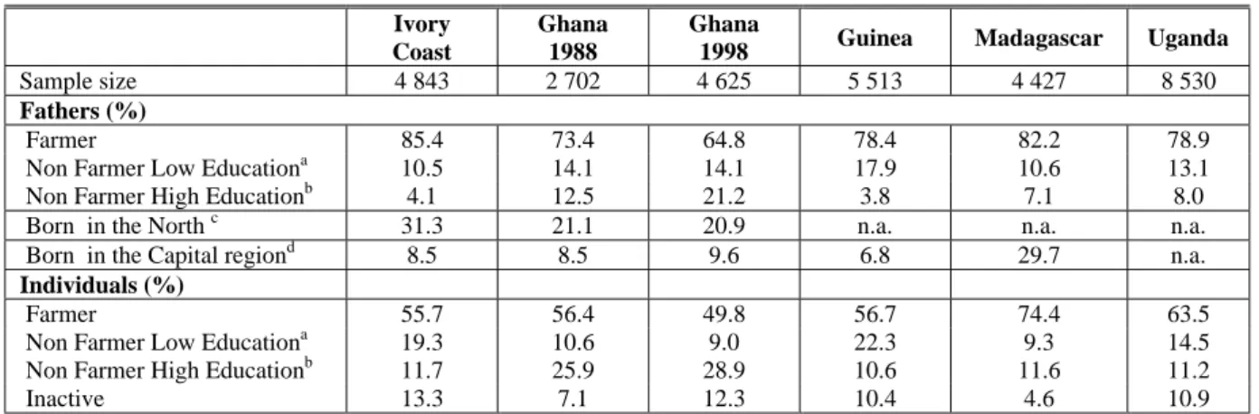
Table 1 shows the size and the breakdown of the five samples by social origins and social positions5. Samples are quite large from 2,700 (Ghana 1987-88) to 8,530 observations (Uganda).
Most of the fathers of 20-69 year old men are farmers, even if there is some variation from the Ivory Coast and Madagascar cases (more than 80%), through Guinea and Uganda (around 78%), to Ghana with only 73% in 1988 and 65% in 1998. In the generation of sons, the share of farmers is still higher than 50% everywhere, except that we observe some divergence across time due to the speed of urbanization. In Madagascar, the share of farmers among sons (74%) is still close to that among fathers (82%), whereas in Ivory Coast we observe a 30 percentage points fall, from 85 to 55%. Although it is slowing down, this structural change is still rapid in some countries, as we see that in Ghana this share fell by 6 percentage points over a decade (1988-98).
Regarding the two other classes of origin and the distribution of education levels, Ghana stands out as the country where secondary education is the most widespread among fathers as well as among sons. In Ghana, middle school level is in fact more like an upper primary level. For the generations concerned (the system was reformed in 1987), the Ghanaian education system offered much longer schooling than elsewhere based on the “6-4-5-2” format: six years in primary school, four in middle school, five years in secondary school and two pre-university years (lower sixth and upper sixth). Individuals could pass an exam to go directly from primary to secondary school, cutting out middle school. However, since primary school had no system of repeating a failed year, half of the individuals (those who had at least reached middle school) had at least completed these six years of schooling. Most of the other half had never attended school, with only a small minority having left school at primary level.
Even before independence, Madagascar and Uganda experienced an early start in primary schooling, due to the policies of Merina and Buganda kingdoms and in particular the openness to European missionaries. Yet this advantage does not give rise to a high proportion of individuals completing primary school and disappears completely at the secondary level when compared with Ghana. In Madagascar and Uganda, two-thirds of individuals aged 20 and over had successfully completed one
5
year of primary education, but very few had completed all five (Madagascar, “5-4-3”) or seven (Uganda, “7-4-2”) years of this level.
At the other extreme, Ivory Coast and even more so, Guinea, stand out as countries where primary education was reserved to a small minority before independence. In fact, Madagascar makes an exception among former French colonies: a continental overview confirms the British colonies’ large advantage in terms of school extension before 1960 (Benavot and Riddle, 1988). While being still behind in terms of access to school in the 1970s, Ivory Coast and Guinea had caught up with Madagascar and Uganda at the middle (“collège” in the French-origin systems) and secondary levels, as is revealed by the sons’ education levels distribution.
Table 1:
Sample description
Ivory Coast
Ghana 1988
Ghana
1998 Guinea Madagascar Uganda
Sample size 4 843 2 702 4 625 5 513 4 427 8 530
Fathers (%)
Farmer 85.4 73.4 64.8 78.4 82.2 78.9 Non Farmer Low Educationa 10.5 14.1 14.1 17.9 10.6 13.1 Non Farmer High Educationb 4.1 12.5 21.2 3.8 7.1 8.0 Born in the North c 31.3 21.1 20.9 n.a. n.a. n.a. Born in the Capital regiond 8.5 8.5 9.6 6.8 29.7 n.a.
Individuals (%)
Farmer 55.7 56.4 49.8 56.7 74.4 63.5 Non Farmer Low Educationa 19.3 10.6 9.0 22.3 9.3 14.5 Non Farmer High Educationb 11.7 25.9 28.9 10.6 11.6 11.2 Inactive 13.3 7.1 12.3 10.4 4.6 10.9
Coverage: Men 20 to 69 year-old.
Sources: Ivory Coast LSMS 1985-1988; Ghana GLSS 1987-88 and 1998; Guinea, EIBC 1994; Madagascar, EPM 1993; Uganda Integrated
Household Survey 1992; calculations by the authors.
a: Low Education: never been at school or has achieved at most primary level. In the case of fathers in Ivory Coast, means having obtained at most a primary degree (CEPE).
b: High Education: having achieved more than primary school level. In the case of fathers in Ivory Coast, means having middle school degree (BEPC).
c: Ivory Coast: born in départements of Bouna, Bondoukou, Boundiali, Dabakala, Ferkessedougou, Katiola, Korhogo, Mankono, Odienné, Séguéla, Tengrela and Touba (20.5%) and born in Burkina-Faso or Mali (10.8%); Ghana: born in regions Northern, Northern West, Northern East.
d. Ivory Coast: Abidjan; Ghana: Greater Accra; Guinea: Conakry; Madagascar: Antananarivo.
The outcome variable is the consumption per head for the household in which the individual lives. In low-income countries, it is more reliable to measure consumption (including home-produced consumption) than income (Deaton, 1997). For each country, consumption components have been meticulously reconstructed from raw survey data using a uniform methodology for comparison purposes6. For the ease of exposition, household consumption per capita is called ‘income’ in the remainder of the paper.
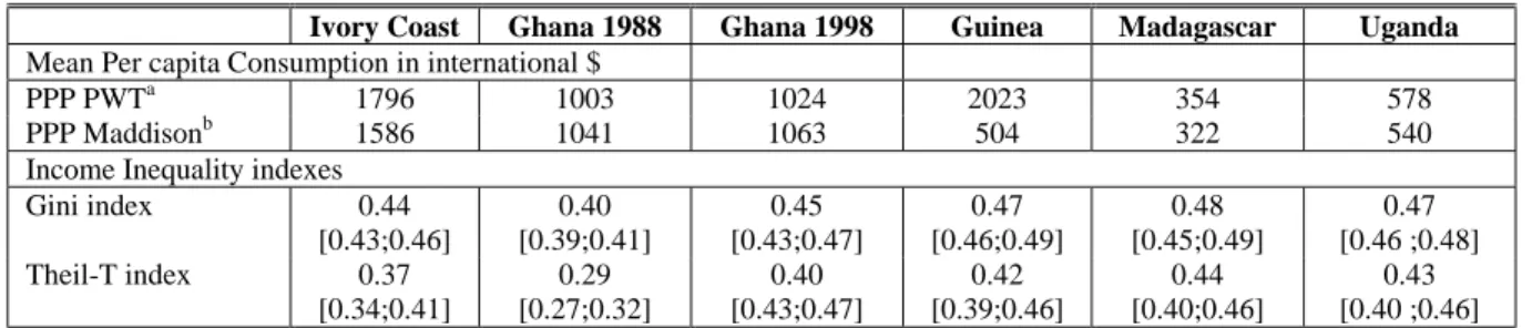
Table 2 first reveals a wide range of mean income levels, once consumption per capita in domestic currency is translated into international dollars using two sources for Purchasing Power Parity (PPP) exchange rates (Heston, Summers and Aten, 2002; Maddison, 2003). The ranking of countries is fairly consistent with GDP in international dollars as estimated by the same sources. 1985-88 Ivory Coast comes out by far as the wealthiest country, followed by Ghana, Uganda and Madagascar. A very large uncertainty regarding price levels in Guinea results in a wide discrepancy between the two income levels estimates for that country; our preference goes to the (much lower) Maddison’s estimate.
6
Details are available from the authors. The consumption variable includes all food and non-food current expenditures, home-produced food consumption, an imputed rent for house owners. It excludes too infrequent expenditures such as durable goods and health, as well as net transfers. It is adjusted for infra-annual inflation. Ghana 1998 consumption is measured at 1988 prices and translated in international dollars using the same PPP exchange rate as Ghana 1987-88.
Table 2: Mean income levels and overall income inequality levels
Ivory Coast Ghana 1988 Ghana 1998 Guinea Madagascar Uganda
Mean Per capita Consumption in international $
PPP PWTa 1796 1003 1024 2023 354 578 PPP Maddisonb 1586 1041 1063 504 322 540 Income Inequality indexes
Gini index 0.44 [0.43;0.46] 0.40 [0.39;0.41] 0.45 [0.43;0.47] 0.47 [0.46;0.49] 0.48 [0.45;0.49] 0.47 [0.46 ;0.48] Theil-T index 0.37 [0.34;0.41] 0.29 [0.27;0.32] 0.40 [0.43;0.47] 0.42 [0.39;0.46] 0.44 [0.40;0.46] 0.43 [0.40 ;0.46]
Coverage: Men 20 to 69 year-old. Sources: see table 1. Notes: Bootstrap confidence intervals between brackets.
a: Per capita consumption in international $ (source Penn World Tables 6.1, PPP level of consumption for the reference year, except for Ghana 1998 for which the PPP deflator is 1988 one).
b: Per capita consumption in international $ (source Maddison, 2003 for the reference year, except for Ghana 1998 for which the PPP deflator is 1988 one).
All five African countries exhibit a very high level of income inequality, comparable with Latin American standards7. Our own estimates are broadly consistent with those which are compiled for the
same countries and surveys by the United Nations WIDER database8 and the World Bank report on Equity and Development (World Bank, 2005). Of the five countries studied, Ghana in 1987-88 has by far the lowest income inequality, while Ghana in 1998 and the four other countries cannot be statistically distinguished9. Lorenz curves dominance confirms this partial ranking.
3. RESULTS: DIFFERENCES IN INEQUALITY OF OPPORTUNITY FOR INCOME
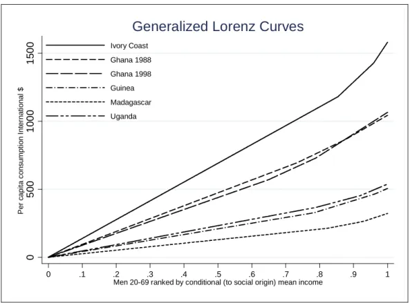
Table 3 shows the maximin index for which both Roemer’s and Van de Gaer’s give the same results, given the monotonicity of the transition matrix linking types of social origins and income. Having a farmer father is always the most disadvantaged social origin, whatever the country that is considered, and whatever the within-type income decile. The index is presented in both its social welfare version (PPP levels with Maddison’s exchange rates) and its inequality (normalized by the mean) version. The social welfare version produces the same ranking of countries as average consumption per capita in PPP (see Table 2): this means that between-countries differences in inequality (of opportunity) are not high enough to modify the differences in income level or poverty. Generalized Lorenz dominance unambiguously confirms this diagnosis (see Figure 1).
7 It should be pointed out that international statistics base most of the estimates for Africa on per capita consumption while most of the
estimates for Latin America are based on per capita income. As income inequality is most often higher than consumption inequality, due to transient components and measurement errors, international comparisons tend to understate the inequality level of Africa in comparison to Latin America.
8 UNU/WIDER–UNDP, 2000. World Income Inequality Database Version 1.0: http://wider.unu.edu/wiid/wwwwiid.htm.
Table 3: Inequality of opportunity for income indexes
Ivory Coast Ghana 1988 Ghana 1998 Guinea Madagascar Uganda
Fathers position in 3 groups
Maximin indexa 1388 946 876 416 258 467 Normalized by mean 0.87 0.91 0.82 0.83 0.80 0.86 Gini index 0.11 [0.10; 0.12] 0.07 [0.07; 0.07] 0.13 [0.12; 0.13] 0.14 [0.14; 0.15] 0.17 [0.16; 0.18] 0.11 [0.11; 0.12] Theil-T index 0.045 [0.042; 0.049] 0.012 [0.011; 0.013] 0.033 [0.032; 0.034] 0.052 [0.051; 0.055] 0.087 [0.083; 0.094] 0.040 [0.038; 0.043] Adding region of birth: Born in the capital town district (6 groupsb)
Maximin indexa 1339 940 858 412 251 n.a. Gini index 0.13 [0.12;0.14] 0.08 [0.07;0.08] 0.15 [0.14;0.15] 0.15 [0.14;0.15] 0.18 [0.17;0.19] n.a. Theil-T index 0.050 [0.047; 0.054] 0.015 [0.014; 0.017] 0.045 [0.043; 0.047] 0.056 [0.054; 0.059] 0.092 [0.086; 0.97] n.a.
Adding region of birth: Born in the North, in the capital town (5 groupsc)
Maximin indexa 1157 804 574 n.a. n.a. n.a. Gini index 0.15 [0.15; 0.16] 0.09 [0.09; 0.10] 0.17 [0.16; 0.17]
n.a. n.a. n.a.
Theil-T index 0.054 [0.051;0.057] 0.016 [.015; .016] 0.049 [0.047; 0.051]
n.a. n.a. n.a.
Coverage: Men 20 to 69 year-old. Sources: see table 1. Notes: Bootstrap confidence intervals between brackets.
a: Per capita consumption in international $ (source Maddison, 2003 for the reference year, except for Ghana.
b: Social origins (3 groups) X being or not being born in the capital town district 1998 for which the PPP deflator is 1988 one).
c: Father Farmer and being born in the North; Father Farmer and being born in the capital town district; Father Farmer and being born elsewhere; Uneducated Non Farmer Father, Educated Non Farmer Father.
Figure 1: Generalized Lorenz Curves between 3 groups of Fathers’ position
0 50 0 10 0 0 15 00 P e r c a pi ta c onsum pt ion In te rnat ional $ 0 .1 .2 .3 .4 .5 .6 .7 .8 .9 1
Men 20-69 ranked by conditional (to social origin) mean income Ivory Coast Ghana 1988 Ghana 1998 Guinea Madagascar Uganda
Generalized Lorenz Curves
Source: ICA Madagascar and Mauritius 2005.
The normalized index gives another ranking of countries: 1987-88 Ghana comes first, followed by Ivory Coast, Uganda, 1998 Ghana, Guinea and lastly Madagascar. For instance, it expresses that the mean income of sons with a father farmer reaches 91% of the country mean income in Ghana, whereas the same ratio is only 80% in Madagascar. These indexes are composed of two basic elements: the first is the earnings scale between social origins, shown in Table 4; the second is the vector of weights of social origins in the population, shown in Table 1. Table 4 reveals that it is in 1987-88 Ghana that mean income differentials by social origins are the lowest, and in Madagascar the highest. In 1987-88 Ghana, the earnings scale goes from 100 through 127 to 151, while in Madagascar it climbs from 100 through 185 to 317.
Table 4: Conditional means differences
Ivory Coast Ghana
1988 Ghana 1998 Guinea Madaga-scar Uganda (1) Father Farmer 100 100 100 100 100 100 (2) F. N-farm.Low E. 170* 127* 130* 184* 185* 146* (3) F. N-farm.High E. 270* 151* 181* 262* 317* 228* F test (2)=(3) (p value) 0.00 0.01 0.00 0.00 0.00 0.00
Coverage: men 20 to 69 year-old. Sources: see table 1. Notes: * significant at 1%.
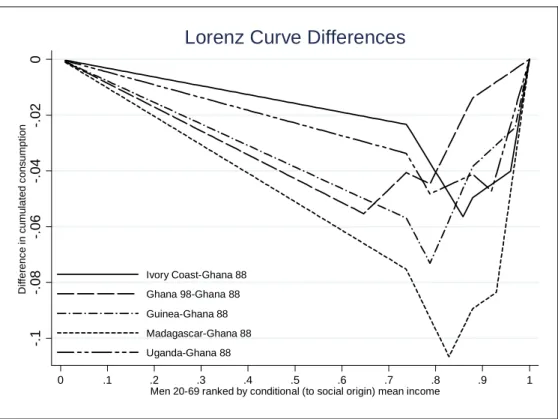
The inequality of opportunity partial ordering provided by Lorenz curves dominance distinguishes only three groups of countries: the two extreme cases, 1987-88 Ghana and 1993 Madagascar, and the group formed by the four other country cases whose Lorenz curves cross each other.
Figure 2: Lorenz Curves between 3 groups of Fathers’ position
-.1 -.0 8 -.0 6 -.0 4 -.0 2 0 D if fer e n c e in c u m u lat e d c o ns umpt ion 0 .1 .2 .3 .4 .5 .6 .7 .8 .9 1
Men 20-69 ranked by conditional (to social origin) mean income Ivory Coast-Ghana 88
Ghana 98-Ghana 88 Guinea-Ghana 88 Madagascar-Ghana 88 Uganda-Ghana 88
Lorenz Curve Differences
This dominance result is reflected in the top panel of Table 3 by the different orderings obtained within the middle-group of countries, according to which inequality index I is chosen to implement the Van de Gaer formula (2). According to the Gini index, Ivory Coast is the second least unequal country followed by Uganda, 1998 Ghana and Guinea, whereas according to the Theil-T index it is 1998 Ghana that comes second, followed by Uganda, Ivory Coast and Guinea. Furthermore, when looking at confidence intervals, only the relative position of Guinea seems statistically reliable for these two indexes.
The second and third panels of Table 3 provide another set of results about the influence of the individuals’ region of birth.
The middle panel shows that being born in the capital town district (interacted with father’s occupation and education level) does not give rise to a very significant advantage and thus does not modify very much the diagnosis about inequality of opportunity, whatever the country that is considered (in Uganda, the region of birth is not available).
In the bottom panel, we additionally distinguish the Northern region of birth category that is most relevant in the cases of Ghana and Ivory Coast (including born in Burkina-Faso or Mali for the latter). It comes out that being born in the Northern disadvantaged regions significantly restricts income opportunities in Ivory Coast and 1998 Ghana. The analysis of the 1988-1998 period of economic recovery in this latter country has indeed revealed that growth resumption has not been evenly distributed between the North and the South (Shepherd and Gyimah-Boadi, 2005)10. In the case of
Ivory Coast, this lack of opportunity of Northerners is one element of explanation for the political crisis that has lead to the partition of the country since 2002 and is not yet entirely solved. It is for 1998 Ghana that this dimension comes out as most meaningful.
In the end, the ordering of countries in three classes seems robust. This ordering suggests that inequality of opportunity for income is only imperfectly correlated with average wealth: although Madagascar is the poorest of our set, Ghana is not the most affluent country when compared to Ivory Coast. Countries’ ranks are more consistent with overall income inequality: Table 2 indeed shows that 1987-88 Ghana is the country with the most equal income distribution, with a Gini index of 0.40, while Madagascar stands out as the most unequal. Furthermore, a look at Ghana across time suggests that economic recovery was accompanied with an increase in both overall inequality and inequality of opportunity.
The last part of our results introduces the social position as an intermediary variable for analyzing the link between social origin and income. As already mentioned in section 2, we coded the sons’ social position as the fathers’, except for an inactive class that gathers students in younger cohorts, unemployed, and retired people in older cohorts. The distribution of population among the four social positions for each country was already given in Table 1.
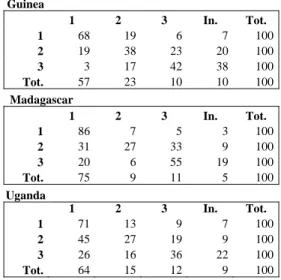
Table 5: Intergenerational social mobility: outflow tables
Ivory Coast Guinea
1 2 3 In. Tot. 1 2 3 In. Tot.
1 63 18 9 10 100 1 68 19 6 7 100
2 17 37 20 26 100 2 19 38 23 20 100
3 5 13 38 44 100 3 3 17 42 38 100
Tot. 56 20 12 13 100 Tot. 57 23 10 10 100
Ghana 1988 Madagascar
1 2 3 In. Tot. 1 2 3 In. Tot.
1 67 10 19 4 100 1 86 7 5 3 100
2 30 21 39 10 100 2 31 27 33 9 100
3 27 5 52 16 100 3 20 6 55 19 100
Tot. 57 11 26 7 100 Tot. 75 9 11 5 100
Ghana 1998 Uganda
1 2 3 In. Tot. 1 2 3 In. Tot.
1 66 8 19 7 100 1 71 13 9 7 100
2 33 18 36 13 100 2 45 27 19 9 100
3 16 4 54 25 100 3 26 16 36 22 100
Tot. 50 9 29 12 100 Tot. 64 15 12 9 100
Coverage: men 20 to 69 year-old. Sources: see table 1. Notes: Father’s position in rows, Son’s positions in columns. 1: Farmer.
2: Non-Farmer with no more than primary education.
10 In fact, our data shows no growth of average consumption per capita over the period. This feature is in line with national accounts data
collected by World Bank (World Development Indicators, 2006). This data combines a positive GDP per capita growth (coming from investment and exports) with a stabilization of consumption per capita.
3: Non-Farmer with post-primary education In.: Inactive (student, unemployed, retired…)
Table 5 shows the outflow tables of intergenerational mobility between social origins and social positions. Conditional probabilities are somewhat difficult to compare at face value, as the weights of each social destination vary from one country to another. However, the share of farmers among sons is roughly comparable between Ivory Coast, Ghana and Guinea. Then, the comparison of the first columns of the corresponding outflow tables reveals that non-farmer sons have a higher probability of working in agriculture in Ghana than in the two other countries. Once the higher weight of farmers is taken into account, the other former British colony, Uganda, shares this characteristic with Ghana. The outflow table for Madagascar reveals two other specific features: a very low rate of exit from agriculture for farmers’ sons and also the highest rate of reproduction in the non-farmer educated social class.
Table 6 presents another element of our decomposition: the earnings scales according to social position. Like for earnings scales according to father’s position, Ghana again stands out with the narrowest earnings scales whatever the year (1988 or 1998) considered. As already noticed in previous works using the same surveys, returns to education are fairly limited in that country (Glewwe and Twum-Baah, 1991; Schultz, 1999; Cogneau et al., 2006). Among other countries, Guinea exhibits the widest earnings scale, while the three remaining countries are rather close to each other from that point of view. The between-groups component of the Theil-T index decomposition tells a rather similar story: while in Ghana income differentials between social positions hardly explain more than 10% of income inequality between 20-69 year old men, in all other countries this share exceeds 20% and reaches 31% in the case of Guinea.
Table 6: income differences between sons according to social positions
Ivory Coast Ghana 1988 Ghana 1998 Guinea Madaga-scar Uganda
(1) Farmer 100 100 100 100 100 100 (2) Non-farmer Low Educ. 158* 136* 138* 236* 173* 200*
(3) Non-farmer High Educ. 321* 157* 199* 368* 314* 285* (4) Inactive 192* 106 149* 208* 214* 198* Between group component of
Theil-T (%) 27 7 12 31 25 21 Coverage: men 20 to 69 year-old. Sources: see table 1.
* Difference with (1) significant at 1%.
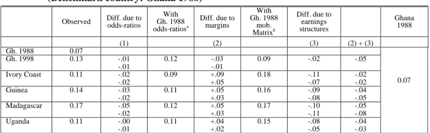
We lastly turn to the decomposition exercises. Table 7 (resp. Table 8) shows in columns the three terms of decomposition of equation (6) when passing from a given country to 1988 Ghana (resp. 1993 Madagascar), the country where inequality of opportunity for income has been estimated as the lowest (resp. the highest). For each pair wise comparison, the two rows correspond to the two possible paths for implementing the same decomposition in the same order: the first row simply starts from the country indicated in the row first column, whereas the second starts from the chosen benchmark country (Ghana 1988 or Madagascar).
Table 7: Decomposition of inequality of opportunity: the impact of mobility matrices
(Benchmark country: Ghana 1988)
Observed Diff. due to odds-ratios
With Gh. 1988 odds-ratiosa Diff. due to margins With Gh. 1988 mob. Matrixb Diff. due to earnings structures Ghana 1988 (1) (2) (3) (2) + (3) Gh. 1988 0.07 0.07 Gh. 1998 0.13 -.01 0.12 -.03 0.09 -.02 -.05 -.01 -.01 Ivory Coast 0.11 -.02 0.09 +.09 0.18 -.11 -.02 -.02 +.05 -.07 -.02 Guinea 0.14 -.03 0.11 +.05 0.16 -.09 -.04 -.02 +.03 -.08 -.05 Madagascar 0.17 -.05 0.12 +.05 0.17 -.10 -.05 -.02 +.03 -.11 -.08 Uganda 0.11 -.00 0.11 +.04 0.15 -.08 -.04 -.01 +.02 -.05 -.03 Coverage: men 20 to 69 year-old. Sources: see table 1.
a: Inequality of opportunity index obtained through a reweighting of observations according to a counterfactual social mobility matrix with the same margins (distribution of father’s and son’s positions) as the country under review but Ghana 1988 odds-ratios.
b: Inequality of opportunity index obtained through reweighting of observations according to the Ghana 1988 social mobility matrix (both odds-ratios and margins).
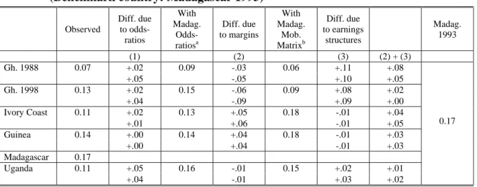
Table 8:
Decomposition of inequality of opportunity: the impact of mobility matrices
(Benchmark country: Madagascar 1993)
Observed Diff. due to odds-ratios With Madag. Odds-ratiosa Diff. due to margins With Madag. Mob. Matrixb Diff. due to earnings structures Madag. 1993 (1) (2) (3) (2) + (3) Gh. 1988 0.07 +.02 0.09 -.03 0.06 +.11 +.08 0.17 +.05 -.05 +.10 +.05 Gh. 1998 0.13 +.02 0.15 -.06 0.09 +.08 +.02 +.04 -.09 +.09 +.00 Ivory Coast 0.11 +.02 0.13 +.05 0.18 -.01 +.04 +.01 +.06 -.01 +.05 Guinea 0.14 +.00 0.14 +.04 0.18 -.01 +.03 +.00 +.04 -.01 +.03 Madagascar 0.17 Uganda 0.11 +.05 0.16 -.01 0.15 +.02 +.01 +.04 -.01 +.03 +.02
Coverage: men 20 to 69 year-old. Sources: see table 1. Notes: see table 7, replace Ghana 1988 by Madagascar 1993.
The first term corresponds to the influence of the mobility matrices inner structure, i.e. odds-ratios. As revealed by the signs of the first term, Ghana (especially in 1988) and Uganda are the countries where intergenerational mobility is the most fluid, and Madagascar where it the most rigid, at least from the standpoint of income opportunities; Ivory Coast and Guinea stand in-between.
The second term assesses the impact of moves in the margins of the mobility tables; it is linked to the differences in economic structures (weight of agriculture) and in educational development. The third term of the decomposition, that we call the earnings structure effect, corresponds to the moves in average earnings attached to each cells of the mobility matrices. The two terms have in most cases large magnitudes. They also have opposite signs, the only exception arising in the historical evolution of Ghana over the 1990s. This latter feature suggests the presence of compositional and/or general equilibrium effects linking labor supply composition to earnings structures.
Because of this general equilibrium issue, we also look at the sum of the second and third terms, and compare column (1) with column (2)+(3). In most cases, the earnings structure effect dominates the margins effect in their sum; or in the Bourguignon, Ferreira and Leite (2002) terminology, price effects dominate population effects, one exception arising when Ivory Coast and Guinea are compared to Madagascar.
When comparing Uganda or 1998 Ghana with Madagascar, the mobility effect dominates the sum of the tables’ margins (population) and earnings structure (price) effects. It also contributes to half of the difference between 1988 Ghana and 1985-88 Ivory Coast (and between 1987-88 and 1998 Ghana for one path). In the other cases, it is dominated by the joint influence of population distribution and earnings structure. However, mobility effects always have the same sign as the sum of population and earnings effects. This latter feature once again suggests that compositional effects and /or general equilibrium forces may be at play that would determine at the same time the earnings differentials, the occupational and educational structure and the intergenerational opportunities.
CONCLUSION
A new analysis of large-sample surveys in five comparable Sub-Saharan African countries, all providing information on individuals’ parental background and region of birth, allows measuring for the first time inequality of opportunity for income in five comparable countries of Africa: Ivory Coast, Ghana, Guinea, Madagascar and Uganda. We compute inequality of opportunity indexes in keeping
with the main proposals in the literature, and propose a decomposition of between-country differences that distinguishes the respective impacts of intergenerational mobility between social origins and positions, of the distribution of education and occupations in the sons’ generation, and of the earnings structure. Among our five countries, Ghana in 1988 has by far the lowest income inequality between individuals of different social origins, while Madagascar in 1993 displays the highest inequality of opportunity from the same point of view. Ghana in 1998, Ivory Coast in 1985-88, Guinea in 1994 and Uganda in 1992 stand in-between and can not be ranked without ambiguity.
Inequality of opportunity for income seems to correlate with overall income inequality more than with national average income, like in the famous comparison between Sweden and United States undertaken by Björklund and Jäntti (2001). Decompositions reveal that the two former British colonies (Ghana and Uganda) share a much higher intergenerational educational and occupational mobility than the three former French colonies. Further, Ghana distinguishes itself from the four other countries, because of the combination of widespread secondary schooling, low returns to education and low income dualism against agriculture. Nevertheless, it displays marked regional inequality insofar as being born in the Northern part of this country produces a significant restriction of income opportunities.
Intergenerational social mobility, school extension and income dualism are not necessarily independent phenomena, if only through general equilibrium effects. More research is warranted about the long-term dynamics that have brought about this differentiation between countries, and in particular between such close neighbors as Ivory Coast and Ghana. Those long-term dynamics would involve the combined impacts of geography, pre-colonial conditions and colonial powers’ policies, and consecutive or disruptive post-colonial State trajectories.
ACKNOWLEDGEMENTS
This research received funding from the Agence Française de Développement (AFD) Research Department. The authors thank Jean-David Naudet for his support and clever remarks. They also thank Thomas Bossuroy, Philippe De Vreyer, Charlotte Guénard, Victor Hiller, Phillippe Leite, Laure Pasquier-Doumer and Constance Torelli for their contributions in the construction of datasets and their participation in the first stage of this study. The usual disclaimer applies.
APPENDICES
Appendix 1: Decomposition of inequality of opportunity indexes using the log-Linear model
The log-linear model provides a useful parameterization of a contingency table such as each country c social mobility tables (Bishop, Fienberg and Holland, 1975).
( )
[
p
cs
,
o
]
c c( )
o
c( )
s
c( )
s
,
o
ln
=
µ
+
α
+
β
+
γ
(A1)This parameterization is unique under the following constraints:
( )
∑
=
o co
0
α
;∑
( )
=
s cs
0
β
;( )
s
o
o
s c∀
=
∑
γ
,
0
,
;( )
s
o
s
o c∀
=
∑
γ
,
0
,
.In this so-called ‘saturated’, i.e. unconstrained, form, the log-linear is purely descriptive. Its coefficients merely provide an arithmetic decomposition of the table frequencies: µc is equal to the
mean of log joint probabilities, αc(o) and βc(s) characterize respectively row and column marginal
probabilities, and the γc(s,o) characterize the odds-ratios.
For instance, in the case where social origin o and social position s are dichotomic (o=0,1 and s=0,1), i.e. if the social mobility table is a 2 rows and 2 columns matrix, one obtains:
( )
( )
( )
( )
[
]
( )
[
( )
( )
]
( )
[
( )
( )
]
( )
( ) ( )
( ) ( )
0
,
1
1
,
0
1
,
1
0
,
0
ln
4
1
1
,
1
1
,
1
ln
1
,
0
ln
2
1
1
1
,
1
ln
0
,
1
ln
2
1
1
1
,
1
ln
0
,
1
ln
1
,
0
ln
0
,
0
ln
4
1
p
p
p
p
p
p
p
p
p
p
p
p
c c c c c c c c c c c c c c c=
−
+
=
−
+
=
+
+
+
=
γ
µ
β
µ
α
µ
In the general case where social origin and social position are polytomic categorical variables, odds-ratios read:
(
)
[
,
;
'
,
'
]
[
( )
,
(
'
,
'
)
]
[
( )
'
,
( )
,
'
]
ln
OR
cs
o
s
o
=
γ
cs
o
+
γ
cs
o
−
γ
cs
o
+
γ
cs
o
(A2)A ‘non-saturated’, i.e. constrained, version of the log-linear model allows us to construct a fictional mobility table where row and column marginal probabilities are those of country c and odds-ratios are those of country c’:
( )
[
pc c s,o]
c c c c( )
o c c( )
s c( )
s,o ln * * ' ' ' * ' * ' =µ
→ +α
→ +β
→ +γ
→ (A3)Under the assumption that frequency counts nc(s,o) follow a multinomial distribution, this model can be estimated by maximum likelihood. The saturated model for country c’ provides the γc’(s,o) which
characterize the country c’ mobility matrix odds-ratios ORc’. The constrained log-linear model of
equation (A3) provides predicted probabilities of a fictional mobility table with country c marginal distributions and country c’ odds-ratios, and conditional probabilities:
p
c*→c'( )
s
o
=
p
*c→c'( ) ( )
s
,
o
p
co
This allows us to define another counterfactual conditional expectation of income for each social origin o:
( )
∑
(
)
→( )
→=
s c c c c cY
o
E
Y
o
s
p
s
o
M
* ' * ',
(A4)We may last define a second counterfactual conditional expectation of income where conditional probabilities of country c’ are used to weight the earnings structure of country c:
( )
=
∑
(
) ( )
→ s c c c cY
o
E
Y
o
s
p
s
o
M
',
' (A5)Then the decomposition of equation (6) is completely defined.
Appendix 2: Tables
Table A 1: Surveys
Country Name of the survey Period Household sample size for analysis Ivory Coast Enquête permanente auprès des ménages (EPAM)
Côte d’Ivoire Living Standards Surveys (CILSS)
Feb.85-Apr.89(a) 4,090 Ghana Ghana Living Standards Survey, rounds 1 and 4
(GLSS1 and GLSS4)
Sep.87-Jul.88 Ap. 98-March 99
3,148 5,923 Guinea Enquête intégrale sur les conditions de vie des ménages
(avec modules budget et consommation) (EIBC)
Jan.94-Feb.95 3,971 Madagascar Enquête permanente auprès des ménages (EPM) Apr.93-Apr.94 3,700 Uganda National Integrated Household Survey (NHIS) Mar.92-Mar.93 8,205
(a): The four surveys approximately cover the whole period. In the first three years, half of the sample has been interviewed again the following year (panel data). For panelized households, only the most recent information was kept, so that the final stacked sample contains around 800 households for each year of the 1985-87 period and 1,600 for 1988-89.
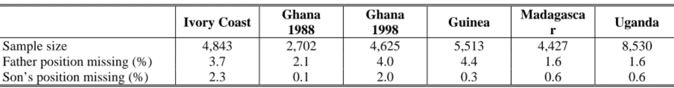
Table A 2: Sample size and missing social origins and social positions
Ivory Coast Ghana
1988 Ghana 1998 Guinea Madagasca r Uganda Sample size 4,843 2,702 4,625 5,513 4,427 8,530 Father position missing (%) 3.7 2.1 4.0 4.4 1.6 1.6 Son’s position missing (%) 2.3 0.1 2.0 0.3 0.6 0.6
REFERENCES
Benavot A. and Riddle P. (1988), “The Expansion of Primary Education, 1870-1940: Trends and Issues”, Sociology of Education, vol. 61, n°3, pp. 191-210.
Bishop Y., Fienberg S. and Holland P. (1975), Discrete Multivariate Analysis: Theory and Practice, Cambridge MA: MIT Press.
Björklund A. and Jäntti M. (2001), “Intergenerational Income Mobility in Sweden Compared to the United States”, American Economic Review, vol.87, n°5, pp. 1009-1018.
Blinder A. S. (1973), “Wage Discrimination: Reduced Form and Structural Estimates”, Journal of
Human Resources, vol. 8, n°4, pp. 436-455.
Bourguignon F., Ferreira F.H.G. and Leite P. (2002), “Beyond Oaxaca-Blinder : Accounting for Differences in Household Income Distributions Across Countries”, DELTA Working Paper, n°2002-04; William Davidson Institute Working Paper n°478; World Bank Working Paper n°2828.
Bourguignon F., Ferreira F.H.G. and Menendez M. (2007), “Inequality of Opportunity in Brazil”,
Review of Income and Wealth, vol. 53, n°4, pp. 585-618.
Chesher A. and Schluter C. (2002), “Welfare Measurement and Measurement Error”, Review of
Economic Studies, vol. 69, pp. 357-378.
Cogneau D. (2006), “Equality of opportunity and other equity principles in the context of developing countries”, in Kochendorfer-Lucius, G. and Pleskovic, B. (Eds), Equity and Development, InWent / World Bank Berlin workshop series, World Bank publications, Washington DC, pp. 53-68.
Cogneau D., Bossuroy T., De Vreyer P., Guénard C., Hiller V., Leite P., Mesplé-Somps S., Pasquier-Doumer L. and Torelli C. (2006), “Inequalities and Equity in Africa”, Working paper DIAL DT 2006-11 and AFD Notes et Documents 31.
Cogneau D. and Gignoux J. (2008), “Earnings Inequalities and Educational Mobility in Brazil over Two Decades”, forthcoming in Klasen, S. and Nowak, F. (Eds.), Poverty, Inequality and Policy in
Latin America, CESifo Series, Harvard, Mass.: MIT Press.
Deaton A. (1997), “The Analysis of Household Surveys: A Microeconometric Approach to Development Policy”, Johns Hopkins University Press, World Bank, August.
Deininger K. and Squire L. (1996), “A New Data Set Measuring Income Inequality”, The World Bank
Economic Review, vol. 10, n°3, pp. 565-591.
Di Nardo J., Fortin N. and Lemieux T. (1996), “Labor Market Institutions and the Distribution of Wages, 1973-92: A Semiparametric Approach”, Econometrica, vol. 64, n°5, pp. 1001-44.
Dunn C. E. (2007), “The Intergenerational Transmission of Lifetime Earnings: Evidence from Brazil”,
The B.E. Journal of Economic Analysis & Policy, vol. 7, n°2, (Contributions), Article 2.
Gajdos T. and Maurin E. (2004), “Unequal uncertainties and uncertain inequalities: an axiomatic approach”, Journal of Economic Theory, vol. 116, n°1, pp. 93-118.
Glewwe P. and Twum-Baah K. A. (1991), “The Distribution of Welfare in Ghana 1987-99”, LSMS Working Paper n°75, 94 pp.
Heston A., Summers R. and Aten B. (2002) Penn World Table Version 6.1, Center for International Comparisons at the University of Pennsylvania (CICUP).
Juhn C., Murphy K. M. and Pierce B. (1993), “Wage Inequality and the Rise in Returns to Skill”,
Journal of Political Economy, vol. 101, n°3, pp. 410-42.
Lam D. (1999), “Generating Extreme Inequality: Schooling, Earnings and Intergenerational Transmission of Human Capital in South Africa and Brazil”, Research Report, Population Studies Center, University of Michigan.
Leite P., Mc Kinley T. and Osorio R. (2006), “The Post-Apartheid Evolution of Earnings Inequality in South-Africa, 1995-2004”, UNDP International Poverty Centre, WP 32.
Louw M., Van Der Berg S. and Yu D. (2006), “Educational Attainment and Intergenerational Social Mobility in South Africa”, Stellenbosch Economic Working Paper 09/06.
Maddison A. (2003), The World Economy: Historical Statistics. Development Center Studies, Paris: OECD.
Moreno-Ternero J. D. (2007), “On the Design of Equal-Opportunity Policies”, Investigaciones
Económicas, vol. 31, pp. 351-374.
Rodríguez J.G. (2008), “Partial Equality-of-Opportunity Orderings”, Social Choice and Welfare, forthcoming.
Oaxaca R. (1973), “Male-Female Wage Differentials in Urban Labor Markets”, International
Economic Review, vol. 14, n°3, pp. 673-709.
Roemer J. (1996), Theories of Distributive Justice, Cambridge MA: Harvard University Press. Roemer J. (1998), Equality of Opportunity, Cambridge MA: Harvard University Press.
Schultz T.P. (1999), “Health and Schooling Investments in Africa”, Journal of Economic
Perspectives, vol. 13, n°3, pp. 67-88.
Shepherd A. and Gyimah-Boadi E. (2005), “Bridging the north-south divide in Ghana?” Background paper for the 2005 World Development Report, mimeo, World Bank, Washington DC.
Shorrocks A. (1978), “The Measurement of Mobility”, Econometrica, vol. 46, n°5, pp. 1013-1024. Van de Gaer D. (1993), “Equality of Opportunity and Investment in Human Capital”, Catholic
University of Leuven, Faculty of Economics, no. 92.
Van de Gaer D., Schokkaert E., and Martinez M. (2001), “Three Meanings of Intergenerational Mobility”, Economica, vol. 68, n°272, pp. 519-38.
World Bank (2005), World Development Report 2006: Equity and Development, New York : Oxford University Press.