Demand forecast accuracy and performance of inventory policies for multi-level rolling schedule MRP problems

Demand forecast accuracy and performance of

inventory policies under multi-level rolling

schedule environments

∗

N.P. Dellaert

_{J. Jeunet}

_,

January 8, 2003

R´esum´e. Cet article ´etudie la performance de plusieurs r`egles d’approvisionnement pour les syst`emes MRP lorsque l’horizon de planification est glissant et la demande incertaine. L’´etude est r´ealis´ee au moyen de simulations num´eriques extensives et montre qu’il est toujours opportun de r´eduire l’amplitude des erreurs de pr´evision. Bien que l’introduction de l’incertitude elle-mˆeme soit un facteur de d´et´erioration des coˆuts plus d´eterminant que le niveau de cette incertitude (mesur´e par l’ampleur des erreurs de pr´evision), nous montrons que les techniques d’approvisionnement contin-uent d’afficher des performances diff´erentes les unes des autres `a mesure que le niveau d’erreur s’accroˆit. Ceci contredit des r´esultats plus anciens selon lesquels toutes les techniques se valent et sont identiquement inefficaces d`es lors que la demande n’est plus certaine. Cet article fournit ´egalement une description claire de la fa¸con dont la proc´edure d’horizon glissant s’applique aux structures g´en´erales de produits finis (qui autorisent l’existence de composants `a multiplicit´e d’utilisation), aux demandes al´eatoires et d´elais d’approvisionnement positifs.

Mots-cl´e: MRP (planification des besoins en composant), stocks multi-´echelon, techniques d’approvisionnement, horizon glissant, erreurs de pr´evision.

∗_{This research was done while Jeunet was a visiting scholar at the International Institute of}

Info-nomics, PO Box 2606, 6401 DC Heerlen, The Netherlands. Support from this institute is gratefully acknowledged.

†_{Department of Operations Management, Eindhoven University of Technology, P.O. Box 513,}

5600 MB Eindhoven, The Netherlands.

‡_{LAMSADE, CNRS, Universit´e Paris Dauphine, Place de Lattre de Tassigny, 75775 Paris Cedex}

16, France.

§_{Corresponding author. Tel.: +33-1-44-05-41-83; fax: +33-1-44-05-40-91.}

Abstract. Our incentive is to study the behaviour of lot-sizing rules in a multi-level context when forecast demand is subject to changes within the forecast window. To our knowledge, only Bookbinder and Heath (1988) proposed a lot-sizing study in a multi-echelon rolling schedule with probabilistic demands. But their simulation study was limited to two arborescent structures with 6 nodes. By means of an extensive simulation study we show that it is always worth decreasing the error magnitude. This should encourage companies to develop Electronic Data Interchange to ameliorate demand forecast.

Although the presence or absence of forecast errors matters more than the error level, we show that lot-sizing rules exhibit significant differences in their behaviour as the level of error is augmented. This paper also provides a clear description of the rolling procedure when applied to general product structures, probabilistic demand within the forecast window and positive lead times.

Keywords: Material Requirements Planning, multi-level lot-sizing, rolling hori-zon, forecast errors.

1

Introduction

In the last two decades information technologies have been increasingly adopted in supply chains. In the mid 80’s bar code usage spread to other sectors than food sector as its force was to facilitate instantaneous data collection at the point of sale. Later on Electronic Data Interchange (EDI) has been developed to facilitate rapid transmission of large amounts of information between retailers and suppliers. Companies along the supply chain undertake to share sales information or consumer specific queries to increase the accuracy of forecasting and respond quickly to customers’ evolving needs.

Providing manufacturers with comprehensive and accurate data relating to the final customer demand enables sharper demand forecasts. Still unknown is the extent to which forecast errors may be reduced through the use of precise and up-to-date sales information. Forecast errors are often in the range of 30-70% and may be reduced to 10-20% if the company implements voluntarist policies to increase the accuracy of forecasting. With EDI, one can expect an additional decrease of errors.

From an inventory management perspective, the question is whether or not it is worth asking for ever more accurate forecasts if forecast errors of even small mag-nitude have a tremendous impact on the cost effectiveness of lot-sizing techniques in Material Requirements Planning (MRP) systems. In a past simulation study De Bodt and Van Wassenhove (1983) have shown that (even small) forecast errors do not only increase the lot sizing costs in a dramatic way but also tend to homogenize the cost performance of the various lot sizing techniques: they tend to perform equally bad. The study was conducted in single-level MRP on a rolling horizon and forecast errors were injected within the forecast window.

The purpose of this paper is to investigate the impact of forecast errors on the performance of several lot-sizing techniques in a multi-level environment on a rolling horizon basis. Our objective is to establish whether or not De Bodt and Van Wassen-hove’s conclusions are still valid in multi-level MRP systems. Previous research deal-ing with multi-level problems under rolldeal-ing conditions rarely considers component commonality and always assumes zero lead times. However, positive lead times and general product structures make the application of the rolling procedure substantially harder and raise infeasibility problems even when demand is known with certainty within the forecast window. The present study offers a detailed presentation of the procedure through illustrations followed by a formal description of the main steps of the procedure.

The paper is organized as follows. Section 2 is dedicated to a literature overview on inventory policies under rolling conditions. Section 3 provides a detailed description of the multi-level lot-sizing problem in a rolling-schedule environment. We discuss the impact of positive lead times and component commonality on the feasibility of production schedules. Section 4 presents the experimental framework designed to assess the impact of forecast errors on the cost effectiveness of various lot-sizing techniques. Section 5 comments on the results of this study. Major conclusions are drawn in Section 6.

2

Literature overview

Research on lot-sizing decisions in MRP systems has essentially focused on the devel-opment of single-level and multi-level heuristics for solving problems with determinis-tic demand over finite horizons. However, this stadeterminis-tic framework ignores the common practice of using a rolling schedule. This approach consists in applying a lot sizing rule over a limited number of future periods, the forecast window, for which demand is known either deterministically or probabilistically. In the latter case, in each pe-riod of the window, the actual demand results from the addition of the forecast and an error term. Usually, only the first lot size is implemented and the horizon rolls forward the next decision period. New demands are then revealed, the model is up-dated and the decision of the first period is again enacted. This process is repeated until the final period of the planning horizon is reached.

Optimal methods for single and multi-level problems with a fixed horizon do not necessarily provide an optimal solution in a rolling-schedule environment. On the contrary, several single-level studies have shown that it might be worth using compu-tationally simple heuristics especially when the forecast window is short. Blackburn and Millen (1980) show that the Wagner-Whitin algorithm (1958) can be outper-formed by the Silver-Meal heuristic (1973), notably when the number of known future demand is limited. De Bodt, Van Wassenhove and Gelders (1982), while analyzing the effects of forecast errors within the forecast window on cost performance of sev-eral single-level models, show that it might be worth using the ‘simplistic’ Economic Order Quantity. Aucamp (1985) provides a comparative study of the performance of several lot-sizing rules, also used in combination with a look ahead/look back strat-egy which consists in either increasing or decreasing the lot sizes generated by any rule until no cost improvement can be found. The author experimentally observes the poor performance of the Wagner-Whitin algorithm and the consistently high per-formance of Least Total Cost and Silver-Meal. Bookbinder and Hn’g (1986) show that a modified version of the Silver-Meal heuristic (to deal with sharply decreasing demand patterns) and a heuristic by Bookbinder and Tan (1985)–which combines the Silver-Meal and the Least Unit Cost criteria–yield the best results in most situ-ations. However, the Wagner-Whitin algorithm is the best method for large forecast windows and any demand pattern other than constant demand.

Similar conclusions have been drawn based upon multi-level studies under rolling schedule conditions. Blackburn and Millen (1982) evaluate the cost performance of the Silver-Meal heuristic and the Wagner Whitin algorithm, also used in combina-tion with several cost modificacombina-tions designed to account for interdependencies among stages in assembly structures. Simulation results indicate that in many situations, the Silver-Meal heuristic outperforms the Wagner-Whitin algorithm. Gupta, Keung and Gupta (1992) show that the Silver-Meal heuristic provides lower costs than the Wagner-Whitin algorithm in most cases. In a recent study Simpson (1999) finds that the Silver-Meal heuristic when combined to one of the cost modifications of Blackburn and Millen (1982) provides the lowest cost schedules under short forecast windows. For larger windows however, the Wagner-Whitin algorithm yields better results. This conclusion was already drawn in earlier single-level studies (Blackburn and Millen, 1980, Bookbinder and Hn’g, 1986).

Past results make clear that forecast window length impacts cost performance, mostly because length dramatically affects the first optimal lot size, a phenomenon

called ‘the horizon effect’. An obvious strategy to overcome this difficulty is to lengthen the window W so as to stabilize the first lot size. In practice, future demand data or accurate forecast are available only for a limited number of future periods. The idea is therefore to use available demand data through W and forecast de-mand beyond W . This strategy is only useful when combined to the Wagner-Whitin algorithm as myopic methods ignore additional information and provide identical schedules, be the horizon extended or not. Implementing such a strategy raises the question of when to stop extending the horizon. Extension is naturally discontinued as soon as a planning horizon is obtained. This occurs when the first lot size remains identical in the optimal solution to t-period problems, with t beginning at the next to last regeneration point (period in which ending inventory equals zero) found in the optimal solution to the W -period problem and t ending at W − 1.

Horizon extension approaches have been widely implemented in single-level prob-lems. Carlson, Beckman and Kropp (1982) investigate the impact of extending the horizon on the cost performance of the Wagner-Whitin algorithm and conclude that in some situations the more information the better. Kropp, Carlson and Beckman (1983) propose and test 4 stopping conditions. They conclude that simpler stop-ping rules perform better. More recently, Russel and Urban (1993) show that, with horizon extension, the Wagner-Whitin algorithm beats the Silver-Meal heuristic for moderate to large window values. For small W -values horizon extension does not help the Wagner-Whitin algorithm to seek improvements over the Silver-Meal heuristic. Refinement of the horizon extension principle has been brought by Stadtler (2000) who proposes a cost modification to be used with the Wagner-Whitin algorithm so as to account for the fictitious aspect of demand data beyond the forecast window. The idea is to assign to a lot size a cost which is proportional to the periods the order covers falling within the forecast window. Stadtler expects this modification to favour more orders in later periods. The resultant look-beyond model yields the best overall results when compared to the Silver-Meal technique and the heuristic of Groff (1979).

As already mentioned, the first optimal lot size stabilizes when a planning horizon is found. Chand (1982) has designed a simple decision rule to select the first lot size whenever a planning horizon is not found. The rule consists in choosing the first lot size with a minimum cost per period. The set of first lot sizes is provided by solving optimally all t-period problems, with t = 1, . . . , W . The computational study indicates that the modified algorithm exhibits a better behaviour than the Wagner-Whitin algorithm and the Silver-Meal heuristic. Later on, Chand (1983) has provided an adaptation of his algorithm to serial systems. Chand is therefore the first author to design a rolling procedure for multi-stage problems even if it is restricted to the very specific serial case.

Despite this abundant relevant literature on the rolling-schedule problem, there is a paucity of research examining multi-level instances with general product structures and positive lead times. Indeed, existing multi-level studies have been restricted to the case of small assembly structures ranging from 5 items to a maximum number of 16 items with zero lead times. The only rolling procedure available in a multi-level context is even confined to the very specific case of serial systems (Chand, 1983). However, common industrial settings often involve large-sized product structures with numerous common parts. Furthermore, the zero lead time assumption is hardly realistic and more restrictive than it seems at first sight. Indeed, implementing lot

sizing decisions on a rolling basis becomes much more complex in this context (i.e. positive lead time and general structures) as lot-sizing methods may provide infeasible schedules due to a lack of component availability.

3

Problem description

3.1

Notation and definition

It is common to represent product structures as directed acyclic graphs (see Book-binder and Koch, 1990, for example). In such a graph each node corresponds to an item and each edge (i, j) between node i and node j indicates that item i is directly required to assemble item j. Node i (equivalently item i) is fully defined by Γ−1(i) and Γ (i) , its sets of immediate predecessors and successors. The set of ancestors —immediate or non-immediate predecessors— of item i is denoted by ˆΓ−1(i). Product structures may be categorized in terms of their complexity index, C, as defined by Kimms (1997). Recall products are numbered in topological order by the integers 1, . . . , P and let P (k) be the number of products at level k, with k = 0, . . . , K (K + 1 is the depth of the structure). The total number of items obviously equals ΣK

k=0P (k), which by definition is also P. The most complex–in the sense of having the largest number of product interdependencies–structure is obtained when each item enters the composition of all the items located at higher levels in the product structure. By contrast, the simplest structure obtains when each item enters the composition of exactly one item belonging to a higher level. Kimms (1997) defines the complexity of a product structure as

C = A − Amin

Amax− Amin

(1) where A = ΣP

i=1|Γ(i)| is the actual number of arcs in the structure. There is of course a minimal number of arcs such as the product structure is connected, which we denote Aminand is equal to P −P (0). Conversely there is a maximum number of arcs denoted Amaxthat the graph can contain with Amax= ΣK−1_k=0{P (k) · ΣK_j=k+1P (j)}. Structures for which the number of arcs equals the minimum number of arcs (A = Amin) are necessarily assembly structures with C = 0 whereas structures such as A = Amax satisfy C = 1. The C-index is therefore bounded from below and above, whereas the traditional index of Collier (1981) is not.

Let Libe the cumulative lead time of item i and liits own lead time (time required to produce or assemble item i). We have

Li= max

j∈Γ−1_(i)(Lj+ lj), (2)

with Li= 0 for all i with no predecessor. As decision periods are the periods in which we order and not the delivery periods, lead time li of item i itself is not included in the definition of Li.

Let W be the forecast window length and T the problem horizon length, with W ≤ T. For each decision period t, lot-sizing rules are applied on time interval R = {t, . . . , min(t + W − 1, T )}, with t = 1, . . . , T and only the first lot size (that of period t) is executed. Within interval R, demand for end items is either known

with certainty or probabilistically. In the latter, demand forecast is subject to error (note the word ‘forecast’ is not used when there is no error). The interval on which lot-sizing rules are applied may be extended to E periods, to increase their efficiency. Interval R becomes R = {t, . . . , t + W − 1, . . . , min(t + E − 1, T )}. Demand in periods t+W, . . . , t+E may be generated with the same pattern as the one utilized in periods t + 1, . . . , t + W − 1. This demand is always fictitious.

Gross requirements di,s for item i in period s ∈ R correspond to the demand that must be satisfied in period s + li. Gross requirements are either forecasted or known with certainty for end items within the forecast window whereas gross requirements for components result from planned orders at higher levels.

Let xi,t be the firm order for item i in period t. It is the number of units of item i which is ordered in period t to fill the net requirements for item i in period t + li.

The pipeline inventory Zi,s represents the amount of inventory for item i at the end of period s if demand di,s is to be satisfied. We have

Zi,s= Zi,s−1+ xi,s− di,s, (3)

with Zi,0= Ii,0.

Inventories and orders reduce the gross requirements to the net requirements. Net requirements bi,s result from the following definition/computation

bi,s= max(0, di,s− Zi,s−1− xi,s). (4)

Once net requirements have been computed in time interval R, any lot-sizing rule is applied on these net requirements so as to obtain planned orders pi,s representing quantities that will possibly be launched in period s. Only the first planned order pi,t is transformed into a firm order xi,t. In other words, we set xi,t = pi,t and xi,t corresponds to a quantity that is really ordered in period t. Planned orders and firm orders are used to compute gross requirements for components as follows

di,s= X j∈Γ(i) ci,j· Xj,s+li with Xj,s+li = ( xj,s+liif s + li< t pj,s+li otherwise , (5)

where ci,j denotes the production ratio (number of units of i to produce one unit of j).

When period T is reached, we are able to compute the inventory Ii,t for all items and periods for cost calculation purposes. We have

Ii,t= Ii,t−1+ ri,t− di,t, (6)

where ri,t denotes the scheduled receipts for item i in period t. Scheduled receipts simply correspond to firm orders after completion, that is ri,t= xi,t−li. Gross

require-ments di,t no longer result from planned orders but from firm orders di,t =

X

j∈Γ(i)

ci,j· xj,t, (7)

3.2

Rolling procedure under certainty

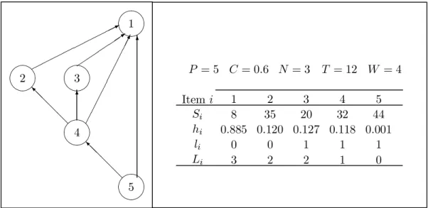
This subsection is dedicated to a description of the rolling procedure applied to general product structures involving positive lead times. We show how a situation of stockout may appear in that situation even if demand is known with certainty within the forecast window. We use a simple example to illustrate the functioning of the rolling procedure. Let us consider the example in Figure 1.

¹¸ º· ¹¸ º· ¹¸ º· ¹¸ º· ¹¸ º· @ @ @ @ I 6 ¢¢ ¢¢ ¢¢ ¢¢¢¸ @ @ @ @ I ´´ ´´´3 ©©©© ©©©© © * 6 1 2 3 4 5 Item i 1 2 3 4 5 Si 8 35 20 32 44 hi 0.885 0.120 0.127 0.118 0.001 li 0 0 1 1 1 Li 3 2 2 1 0 P = 5 C = 0.6 N = 3 T = 12 W = 4

Figure 1: Data of an example

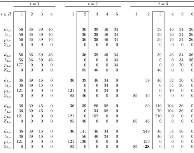
Product structure in Figure 1 involves 5 items with a complexity index equals C = (7 − 4)/(9 − 4) = 0.6. We chose T = 12 and W = 4, which means that we apply any lot-sizing rule on the net requirements for 4 periods of deterministic demand. Lead times are only positive for items 2, 3 and 4. Table 1 exhibits the rolling procedure for the first three periods of the planning horizon. At the beginning, (t = 1), we know the demand for the end item 1 in periods 1 to 4 and we must implement launching decisions for all items in period 1. In this example, we have applied the Wagner-Whitin algorithm in a sequential fashion. The algorithm proposes the lot for lot solution for item 1 and a single lot size for the components. We implement the first lot-sizing decision, so we set xi,1 = pi,1, ∀i. In period 2, a new demand is revealed (that of period 5) so we still know 4 future demands. For the first three items, the Wagner-Whitin algorithm suggests an order in period 5 to cover the new demand. Gross requirements for item 4 have increased in period 3 and 4; a new order is now required in period 3. A similar situation can be observed for item 5. We set xi,2 = pi,2 for all items. In period 3, the Wagner-Whitin algorithm operates on periods {3, 4, 5, 6}. The lot for lot solution is still suggested for the end item. For items 2 and 3, the planned order in period 4 has been increased to cover the new demand of period 6. A single order is still proposed for item 4 in period 3. Given that planned orders in period 3, we may recompute the gross requirements for item 5 in period 2, using formula (5). We have d5,2 = p4,3 + p1,3 = 210 + 39 = 249 but in that period we only have Z5,1+ x5,2 = 85 + 136 = 221 and it is already too late to increase x5,2 for this lot size belongs to the past. The stream of planned orders in period 3 is therefore infeasible as Z5,2= Z5,1+ x5,2− d5,2= 85 + 136 − 249 < 0.

t = 1 t = 2 t = 3 s ∈ R 1 2 3 4 1 2 3 4 5 1 2 3 4 5 6 d1,s 56 36 39 46 36 39 46 34 39 46 34 36 b1,s 56 36 39 46 36 39 46 34 39 46 34 36 p1,s 56 36 39 46 36 39 46 34 39 46 34 36 Z1,s 0 0 0 0 0 0 0 0 0 0 0 0 d2,s 56 36 39 46 36 39 46 34 39 46 34 36 b2,s 56 36 39 46 0 0 0 34 0 0 34 36 p2,s 177 0 0 0 0 0 0 34 0 0 70 0 Z2,s 0 0 0 0 85 46 0 0 46 0 0 0 d3,s 36 39 46 0 36 39 46 34 0 39 46 34 36 0 b3,s 36 39 46 0 0 0 34 0 0 34 36 0 p3,s 121 0 0 0 121 0 0 34 0 0 70 0 0 Z3,s 0 0 0 0 85 46 0 0 0 85 46 0 0 0 0 d4,s 36 39 46 0 36 39 80 68 0 39 116 104 36 0 b4,s 36 39 46 0 0 34 68 0 70 104 36 0 p4,s 121 0 0 0 121 0 102 0 0 210 0 0 0 Z4,s 0 0 0 0 85 46 0 0 0 85 46 0 0 0 0 d5,s 36 39 46 0 36 141 46 34 0 249 46 34 36 0 b5,s 36 39 46 0 56 46 34 0 46 34 0 0 p5,s 121 0 0 0 121 136 0 0 0 136 0 0 0 0 Z5,s 0 0 0 0 85 0 0 0 0 85 -28 0 0 0 0

di,s: gross requirements for item i in period s, bi,s: net requirements, pi,s: planned order,

Zi,s: pipeline inventory.

Table 1: A situation of stockout

We are now able to provide a formal definition of the feasibility of planned orders. A stream of planned orders in period t is feasible (and may be transformed into firm orders) if and only if

Z_i,k−1+ xi,k ≥ di,k ∀ i| Γ(i) 6= ∅ and ∀k ∈ {t − li, . . . , t − 1}. (8) To check this inequality, we only need to recompute the gross requirements in time interval {t − li, . . . , t − 1}, using formula (5).

Each time the above inequality is not satisfied, we face a stockout. The most natural solution to cope with such a situation is to introduce safety stocks at all levels in the product structure. This solution is widely employed in a stochastic context. Whenever a stockout is about to occur the safety stock is increased so as to avoid lost demands. In the above example, a safety stock of 28 units for item 5 would have impeded the stockout exhibited in Table 1. Such a safety stock strategy is obviously implemented at the expense of extra carrying costs.

3.3

Rolling procedure under probabilistic demand

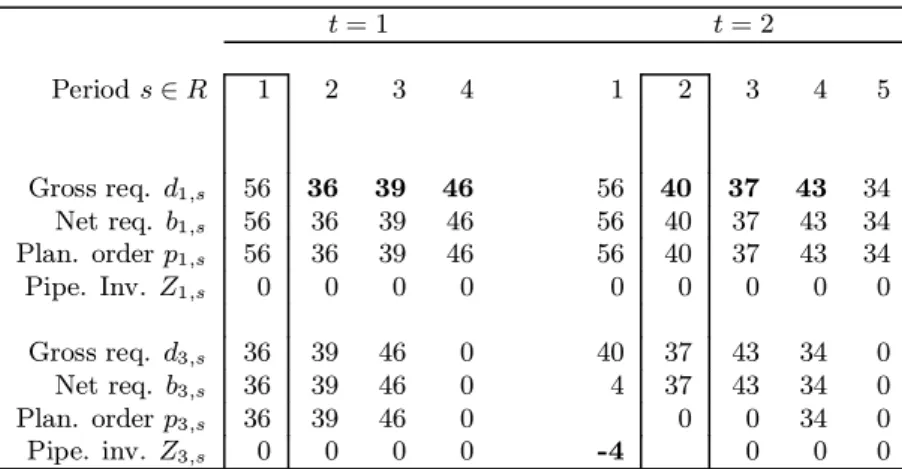
Let us consider our example in Figure 1 and suppose the lot for lot solution is sug-gested for items 1 and 3. It is only necessary to consider these two items to illustrate the functioning of the rolling procedure when demand is not certain. Table 2 displays the procedure for items 1 and 3 for the first two periods of the planning horizon. In period t = 2, demand for item 1 in periods 2, 3 and 4 has changed and the demand in period 5 is now known probabilistically. Demand increase in period 2 triggers a bigger demand for item 3 in period 1 that cannot be covered by a proper order (it is too late). We therefore face a stockout of 4 units of item 3 in period 1.

t = 1 t = 2 Period s ∈ R 1 2 3 4 1 2 3 4 5 Gross req. d1,s 56 36 39 46 56 40 37 43 34 Net req. b1,s 56 36 39 46 56 40 37 43 34 Plan. order p1,s 56 36 39 46 56 40 37 43 34 Pipe. Inv. Z1,s 0 0 0 0 0 0 0 0 0 Gross req. d3,s 36 39 46 0 40 37 43 34 0 Net req. b3,s 36 39 46 0 4 37 43 34 0 Plan. order p3,s 36 39 46 0 0 0 34 0 Pipe. inv. Z3,s 0 0 0 0 -4 0 0 0

Table 2: The occurrence of a stockout under probabilistic demands

This example provides a typical illustration of stockout situations arising when demand forecast is subject to error. Actually, stockouts could be tolerated at the expense of a lower service level. Several lot-sizing rules may provide different results both in terms of cost effectiveness and service levels. As it is tricky to compare them on the basis of these two criteria, we introduce safety stocks for all components so as to make the service level always equal to 100%. Bookbinder and Heath (1988) or Wemmerl¨ov and Whybark (1984) have implemented a search routine for the appro-priate values of safety stocks. First no safety stock is introduced and the maximum stockout is recorded. Second, the safety stock is set to the value of the maximum stockout and the lot-sizing rule is re-applied. The safety stock is adjusted each time a stockout is about to occur. Once the safety stock is large enough, the rule is applied over the whole problem horizon and the cost is computed.

3.4

Formal presentation of the rolling procedure with safety stocks

Table 3 lists the operations to be performed in a rolling schedule environment for all items i in the current period t for which set-up decisions must be implemented. We first recompute the gross requirements and pipeline inventories in past periods {t−li− 1, . . . , t − 1}. In period t−l_P i−1 gross requirements take their final value as di,t−li−1=

j∈Γ(i)

ci,j· xj,t−1 with all xj,t−1 determined in the previous period. This preliminary computation is necessary to determine the net requirements in time interval {t, . . . , t+ W − 1} on which we shall apply any lot-sizing rule so as to obtain a stream of planned orders {pi,s}s=t,...,t+W −1. Computation of net requirements incorporates the

safety stock SSi for each item i. The boolean variable ‘IncludeSS’ ensures that the safety stock is only included in the first planned order of the forecast window W. Once planned orders have been determined along the forecast window, we implement the first lot size decision by setting xi,t = pi,t. This firm order triggers scheduled receipts li period(s) later. When the current period is the first period (t = 1), scheduled receipts are set to a value that makes any solution feasible. By doing so, we ensure production possibilities for all items within the cumulative lead time. When large product structures are considered, cumulative lead times may be so long that nothing is produced for a large portion of the horizon. To smooth away periods with zero production some authors (like Wemmerl¨ov and Whybark, 1984) simply choose to record no statistics for a given number of periods they call the start-up period. Finally, ending inventories are computed and stockouts (SOi,t) are recorded for each item in each period. Values of safety stocks SSi are updated and the full rolling procedure is repeated until no more stockout occurs.

4

Experimental framework

We begin with a brief presentation of the lot-sizing techniques included in the study. We then describe how demand and forecast errors are generated. We finally provide our cost generator and discuss the values of other parameters which were employed in the experiment.

4.1

Lot-sizing procedures

We selected seven single-level lot-sizing rules for use in the study. The Wagner-Whitin algorithm (1958), the Silver-Meal technique (1973), the incremental part period algo-rithm (1968), the Silver version of the economic order quantity (Silver, 1976) and the periodic order quantity. The lot for lot solution was initially included but its extreme performance led us to abandon it. Despite the development of heuristics specifically designed to account for interdependencies among stages, the chosen heuristics are still widely adopted in practice under rolling and multi-level conditions.

The Wagner-Whitin algorithm (WW) provides the optimal solution to the single-level lot-sizing problem by use of dynamic programming. The economic order quan-tity (EOQ) is the traditional Wilson lot-sizing model which balances the inventory carrying costs and order costs. The Silver version of this method lumps an integer number of future demands closest to the EOQ value. The periodic order quantity (POQ) uses the EOQ to determine the reorder time cycle and then orders what is ac-tually forecasted for that time cycle. The incremental part period algorithm (IPPA) increases the size of the order until carrying costs are equal or less than the set-up cost. The Silver-Meal heuristic selects the order quantity so as to minimize the cost per unit time over the time periods the order lasts. The least unit cost (LUC) selects the order quantity so as to minimize the cost per unit (cumulation of the requirements until the cost per unit starts to increase).

4.2

Demand generation

Within the forecast window, demand for end items is defined as ds= ˆds+ εs ∀s = t, . . . , t + W − 1

repeat

for t = 1, . . . , T for i = 1, . . . , P

Computation of d, Z and b for s = t − li− 1, . . . , t − 1

recompute di,s(equation (5))

recompute Zi,s(equation (3))

IncludeSS=true for s = t, . . . , t + W − 1 compute di,s if IncludeSS=true set ∆i = SSi else set ∆i = 0

if Zi,s−1+ xi,s< di,s+ ∆i

bi,s = di,s+ ∆i− Zi,s−1− xi,s

Zi,s= 0

IncludeSS=false else

bi,s = 0

Zi,s= Zi,s−1+ xi,s− di,s

apply any lot-sizing rule on {bi,s}s=t,...,t+W−1

(we thus obtain {pi,s}s=t,...,t+W−1)

set xi,t= pi,t

set ri,t+li = xi,t

Initial values for scheduled receipts if t = 1

for s = 1, . . . , li

ri,s= P j∈Γ(i)

pj,s

Ending inventories and updated safety stocks for i = 1, . . . , P

for t = 1, . . . , T

Ii,t= max(Ii,t−1, 0) + ri,t− di,t

if Ii,t < 0

SOi,t= −Ii,t

else SOi,t= 0 SSi = SSi+ max t=1,...,TSOi,t until P i=1,...,P µ max t=1,...,TSOi,t ¶

= 0 (no more stockout)

Table 3: Rolling procedure with safety stocks

where ˆds is the estimated demand and εs is the forecast error. Although several end items could have been included in the present study we chose to take only one end item per product structure for the sake of simplicity.

4.2.1 Demand patterns

Estimated demands may follow different patterns. We chose to generate demand for the end item from a uniform distribution of mean 50. We have ˆds ∼ U[0, 2d]. Stan-dard deviation of estimated demands therefore equals ¡_{1/12(100 − 0)}2¢1/2= 28.86.

We also chose to generate demands from a normal distribution with same average and standard deviation: ˆds∼ N[50, 28.86].

4.2.2 Forecast errors

We hypothesized εs ∼ N (0, σs) and we selected two patterns for the forecast errors. We first assumed that forecast errors have a constant variance

σs= σ ∀s = t, . . . , t + W − 1 and σ =

n

0.0d, 0.1d, 0.2d, 0.3d, 0.4d, 0.5d, 0.6do. Like De Bodt et al. (1982), we also considered increasing errors with time

σs= (s − t) · σ ∀s = t, . . . , t + W − 1,

with the same values for σ as above. Demand in period t is known with certainty whereas error variance equals σ in the next period, 2σ for two periods ahead and so son. Whenever εs− ˆds< 0, we set ds to zero and the actual demands were adjusted so that the average actual demand was equal to the forecast mean.

4.3

Cost generation

In accordance with the assumption of value-added holding costs, carrying costs for each item were defined as follows

hi = ei+

X

j∈Γ−1(i)

cj,i· hj with ei = 0.0005 + 0.02 × u,

where u is selected from a uniform distribution between 0 and 1.

We used the TBO (time between orders) factor to determine set-up cost param-eters. For each item we set

Si = 0.5 · di· hi· T BO2 with di =

X

h∈Γ(i)

ci,h· dh.

Three levels of TBO were chosen: 2, 4 and 6.

4.4

Other parameters

Lead times were uniformly drawn at random in the set {1, 2}. Product structures were defined in terms of the complexity index C. We chose 4 values of C in the set {0.00, 0.25, 0.50, 0.75}. In the first phase of our experiment, we involved structures with one end item made of 9 components (P = 10), the lowest level was set to 3 throughout and the planning horizon was set to 60 periods. In the second phase, larger problems were generated with P = 50, N = 8. The horizon length was set to 120 periods as in earlier studies (e.g. De Bodt et al. 1982). In both phases the forecast window length was a function of TBO values. Blackburn and Millen (1980) reported that a forecast window of 3 TBO was appropriate for heuristic procedures

whereas Lundin and Morton (1975) suggested that a window of 5 TBO should be used for WW. Consequently, we set W = 3 × T BO and W = 5 × T BO. Each of the 2 × 2 × 7 × 3 × 4 × 2 = 672 experiments was replicated 5 times, therefore providing 3360 cost observations per lot-sizing rule.

5

Simulation results

As already mentioned, the experiment was divided into two phases. The first sub-section presents the simulation results for problems of moderate size in which we included the Wagner-Whitin algorithm. Execution time of WW precluded its use for larger problems. In the first phase, WW was already greedy compared to other techniques. For instance to solve one rolling problem with P = 10 and T = 60, each single-level technique is applied approximately P × T = 600 times and determination of appropriate values for safety stocks requires on average 3 passes or runs of the full rolling procedure. Thus, to get cost observations associated with one technique and one scenario, we need to apply the concerned technique 3 × P × T = 1800 times. For these small instances, it required on average 0.06 sec. for any heuristic other than WW to solve one case (including the determination of safety stock values). Ex-ecution time of WW was 70 times higher with an average of 4.38 sec. per scenario (simulations were run on a Pentium III, 450 Mhz). Thus, despite the development of ever more powerful computers, computational disadvantage of WW is unmistakable under multi-level rolling conditions.

5.1

small instances

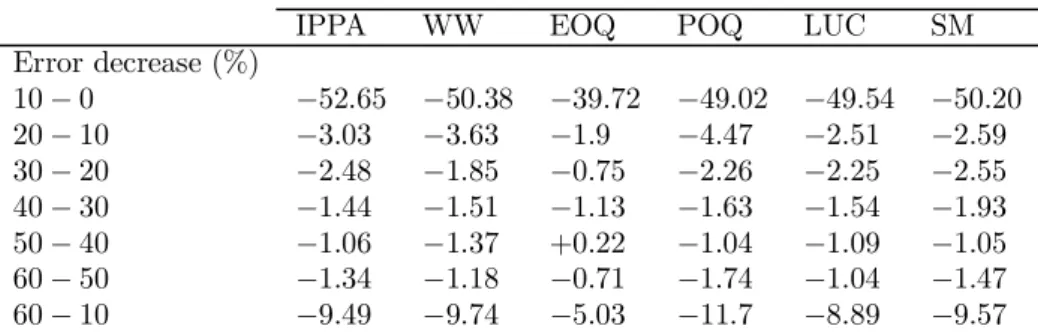
Table 4 gives for any lot-sizing rule the average cost decrease resulting from an error depletion (each entry is an average of 480 observations). For instance, reducing the error from 10% to 0% yields a cost decrease of 52.65% using the IPPA rule. The first row clearly shows that switching from a situation of low error (10%) to a situation of certainty leads to a cost reduction of about 50% whatever the employed technique. Decreasing the error level yields better cost reductions when the initial level of uncertainty is moderate: cost reduction is about 3% for an error decrease from 20% to 10% whereas it approximates 1% for a decrease in uncertainty from 60 to 50% or 50 to 40%. Whatever the selected technique reducing the error level always leads to a significant cost decrease.

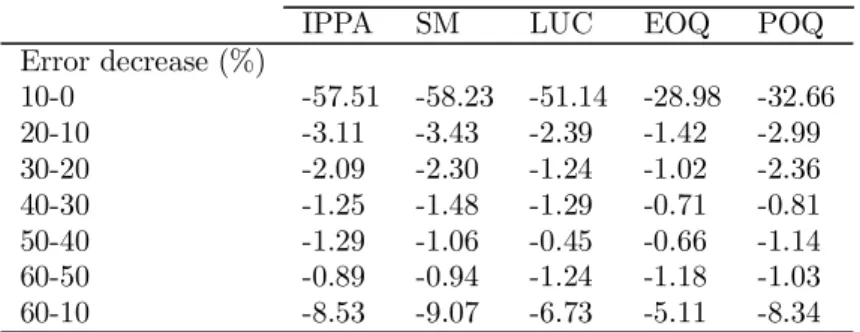
IPPA WW EOQ POQ LUC SM Error decrease (%) 10 − 0 −52.65 −50.38 −39.72 −49.02 −49.54 −50.20 20 − 10 −3.03 −3.63 −1.9 −4.47 −2.51 −2.59 30 − 20 −2.48 −1.85 −0.75 −2.26 −2.25 −2.55 40 − 30 −1.44 −1.51 −1.13 −1.63 −1.54 −1.93 50 − 40 −1.06 −1.37 +0.22 _{−1.04 −1.09 −1.05} 60 − 50 −1.34 −1.18 −0.71 −1.74 −1.04 −1.47 60 − 10 −9.49 −9.74 −5.03 −11.7 −8.89 −9.57

Table 4: Average cost decrease per error decrease

Table 5 provides for each technique the average cost deviation relative to the best overall rule namely IPPA (bold numbers). For each error level we have 2 × 2 × 3 ×

2 × 5 × 4 = 480 cost observations per rule (2 demand patterns, 2 error patterns, 3 TBO values, 2 window lengths, 4 values of the complexity index and 5 replications). In each of these 480 situations we divided the cost of a given technique by the cost provided by IPPA in the same situation and then averaged over the 480 scenarios. Table 5 also gives the standard deviation computed in a similar way (regular numbers below bold numbers). For instance, WW produces costs that are on average 6.95% higher than the costs of IPPA with a standard deviation of 21.36% in case of no error. The last five rows exhibit the result of testing the impact of error levels on the relative cost performance of the heuristics using the non-parametric Kruskal-Wallis ANOVA.

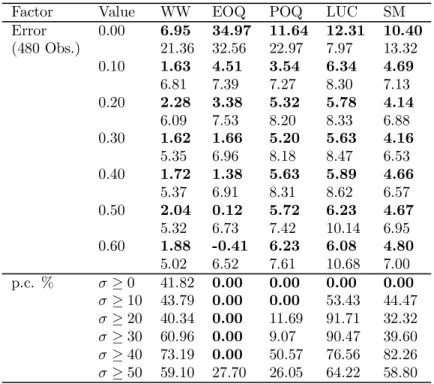
Factor Value WW EOQ POQ LUC SM Error 0.00 6.95 34.97 11.64 12.31 10.40 (480 Obs.) 21.36 32.56 22.97 7.97 13.32 0.10 1.63 4.51 3.54 6.34 4.69 6.81 7.39 7.27 8.30 7.13 0.20 2.28 3.38 5.32 5.78 4.14 6.09 7.53 8.20 8.33 6.88 0.30 1.62 1.66 5.20 5.63 4.16 5.35 6.96 8.18 8.47 6.53 0.40 1.72 1.38 5.63 5.89 4.66 5.37 6.91 8.31 8.62 6.57 0.50 2.04 0.12 5.72 6.23 4.67 5.32 6.73 7.42 10.14 6.95 0.60 1.88 -0.41 6.23 6.08 4.80 5.02 6.52 7.61 10.68 7.00 p.c. % _{σ ≥ 0} 41.82 0.00 0.00 0.00 0.00 σ ≥ 10 43.79 0.00 0.00 53.43 44.47 σ ≥ 20 40.34 0.00 11.69 91.71 32.32 σ ≥ 30 60.96 0.00 9.07 90.47 39.60 σ ≥ 40 73.19 0.00 50.57 76.56 82.26 σ ≥ 50 59.10 27.70 26.05 64.22 58.80

Table 5: Means and standard deviations of cost increases - small instances To highlight the results in Table 5, we chose to plot the average cost deviation from IPPA in Figure 2 for all positive error levels (for σ = 0, cost deviations were too dispersed to be included in the Figure). This figure also provides the results of the Wilcoxon test for paired samples we used to explore differences between lot-sizing rules for each positive error level. The test was performed on gross cost observations and was used to appraise the null hypothesis that the costs produced by two different techniques come from the same distribution. A vertical line linking two points or a squared around two points in Figure 2 means that no statistically significant difference exists between the two concerned techniques at the 5% level.

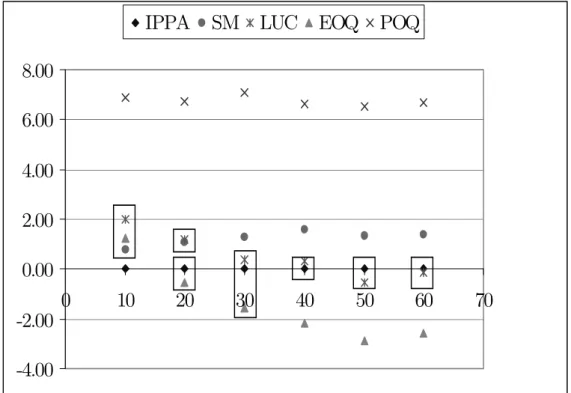
For σ = 0 (no error, see Table 5) IPPA is the best heuristic followed by WW that produces on average cost that are 6.95% higher than those resulting from IPPA. However, the Wilcoxon test revealed that there are no significant differences between IPPA and WW. POQ, SM and LUC produce costs that deviate from IPPA by 10-12% but these heuristics are all different. The worst technique under certainty is EOQ with an average cost deviation of 34.97%.

imme--1.00

0.00

1.00

2.00

3.00

4.00

5.00

6.00

7.00

0

10

20

30

40

50

60

70

IPPA

WW

EOQ

POQ

LUC

SM

Figure 2: Average cost deviation relative to IPPA and Wicoxon test results - small instances.

diately decrease and become less dispersed than they are under certainty. However, significant differences exist between some pairs of rules. WW is the second best heuristic after IPPA. IPPA and WW are different from each other and also from the rest of the techniques. POQ and EOQ are not significantly different and perform worse than IPPA and WW. The worst heuristics are LUC and SM and they are not statistically different from each other.

For σ = 20% to σ = 60%, POQ behaves exactly in the same way as LUC and ex-hibits the poorest performance. SM performs better than LUC and seems to produce better costs than POQ although there are no significant differences between SM and POQ. From Figure 2 it can be seen that these three heuristics exhibit a very similar behaviour for the various levels of error and differences between their cost deviations are clearly steady over the σ-values. Results of the Kruskal-Wallis ANOVA test show that the performance of these three procedures is no longer affected by the magnitude of errors as soon as σ ≥ 20% (critical probabilities in Table 5 for σ ≥ 20% to σ ≥ 50% are all superior to 5%).

WW still appears as the second best method after IPPA for errors up to 30%. As outlined by the ANOVA test (see Table 5) its performance is not affected at all by the introduction of uncertainty. On Figure 2 we can easily observe that WW’s average deviation from IPPA is always around 2% whatever the magnitude of errors. EOQ is the only heuristic whose performance dramatically improves with the level of uncertainty (see Figure 2). This is confirmed by the critical probabilities in Table 5: up to σ = 50% there are significant differences in EOQ’s relative cost performance

from one error level to the next. This result is consistent with prior single-level studies (De Bodt et al., 1982 and Wemmerl¨ov, 1984). Starting with the worst cost deviation from benchmark under certainty, the performance of EOQ gradually improves so as to reach that of WW for σ = 30% and that of IPPA for σ ≥ 50%.

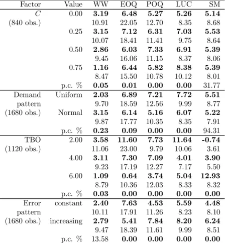
Factor Value WW EOQ POQ LUC SM C 0.00 3.19 6.48 5.27 5.26 5.14 (840 obs.) 10.91 22.05 12.70 8.35 8.68 0.25 3.15 7.12 6.31 7.03 5.53 10.07 18.41 11.41 9.75 8.64 0.50 2.86 6.03 7.33 6.91 5.39 9.45 16.06 11.15 8.37 8.06 0.75 1.16 6.44 5.82 8.38 5.39 8.47 15.50 10.78 10.12 8.01 p.c. % 0.05 0.01 0.00 0.00 31.77 Demand Uniform 2.03 6.89 7.21 7.72 5.51 pattern 9.70 18.59 12.56 9.99 8.77 (1680 obs.) Normal 3.15 6.14 5.16 6.07 5.22 9.87 17.77 10.35 8.35 7.91 p.c. % 0.23 0.09 0.00 0.00 94.31 TBO 2.00 3.58 11.60 7.73 11.64 -0.74 (1120 obs.) 11.06 23.00 9.79 10.06 3.61 4.00 3.11 7.30 7.09 4.01 3.90 9.23 17.19 12.27 7.17 5.50 6.00 1.09 0.64 3.74 5.04 12.93 8.79 10.36 12.03 8.33 8.32 p.c. % 0.03 0.00 0.00 0.00 0.00 Error constant 2.40 7.63 4.53 5.59 4.48 pattern 10.11 17.91 11.26 8.23 8.10 (1680 obs.) increasing 2.79 5.41 7.84 8.20 6.24 9.47 18.39 11.61 9.99 8.51 p.c. % 13.58 0.00 0.00 0.00 0.00

Table 6: Means and standard deviations of cost ratios for other factors and critical probabilities - small instances

Table 6 displays the average cost deviations from IPPA for the other factors in-cluded in the study (C, T BO, ...). These average cost ratios appear in bold numbers and standard deviations are the regular numbers underneath. Table 6 also exhibits the critical probabilities for the Kruskal-Wallis ANOVA test which was used to ap-praise the impact of the various factors on the performance. Product structure com-plexity has a significant effect on the rules’ relative cost performances (apart from SM) but the relationship between complexity and cost ratios is unclear. There is only a tendency for WW to improve as complexity is increased. The choice of a particular demand pattern also impacts on the cost performance except for SM. Cost performance of all heuristics except SM tends to improve as the level of TBO is in-creased. This is possibly due to a wider visibility as forecast windows are increasing with TBO and usually longer windows ameliorate the cost performance. The error pattern exerts influence on the cost performance of all techniques except WW which was already insensitive to the error level. EOQ’s relative cost performance improves for errors increasing in time. EOQ’s relative performance is definitely better with more errors.

5.2

Larger problems

Table 7 is analogous to Table 4 and displays the average cost reduction obtained by gradually diminishing the error level.

IPPA SM LUC EOQ POQ Error decrease (%) 10-0 -57.51 -58.23 -51.14 -28.98 -32.66 20-10 -3.11 -3.43 -2.39 -1.42 -2.99 30-20 -2.09 -2.30 -1.24 -1.02 -2.36 40-30 -1.25 -1.48 -1.29 -0.71 -0.81 50-40 -1.29 -1.06 -0.45 -0.66 -1.14 60-50 -0.89 -0.94 -1.24 -1.18 -1.03 60-10 -8.53 -9.07 -6.73 -5.11 -8.34

Table 7: Average cost decrease per error reduction - larger problems

As expected, reducing the error level from 10% to 0% yields the biggest cost reductions, whatever the employed technique. This reduction approximates 50% for IPPA, SM and LUC whereas it reaches 30% for EOQ and POQ. Again, the cost reduction is always more important when the (initial) error level is moderate.

Like Table 5, Table 8 presents the average cost deviations relative to IPPA, the standard deviations and the results of the Kruskal-Wallis ANOVA test for 50−item product structures over a total number of T = 120 periods.

Factor Value SM LUC EOQ POQ Error 0.00 0.78 16.75 82.69 85.55 (480 obs.) 11.79 10.74 48.70 73.13 0.10 0.77 1.99 1.24 6.88 3.87 6.91 7.00 6.01 0.20 1.10 1.18 -0.56 6.73 3.86 6.24 6.85 5.71 0.30 1.30 0.36 -1.57 7.07 3.67 6.57 7.25 6.15 0.40 1.57 0.33 -2.18 6.62 3.97 5.99 7.16 6.18 0.50 1.35 -0.54 -2.87 6.51 3.77 5.89 6.66 5.83 0.60 1.39 -0.15 -2.57 6.68 3.87 6.24 6.44 5.95 p.c. % _{σ ≥ 0} 0.00 0.00 0.00 0.00 σ ≥ 10 1.31 0.00 0.00 64.69 σ ≥ 20 49.96 0.00 0.00 68.67 σ ≥ 30 83.54 4.46 0.54 67.82 σ ≥ 40 66.50 9.73 26.11 96.70 σ ≥ 50 89.99 58.64 57.01 81.85

Table 8: Means, standard deviations of cost increases and ANOVA test results -larger problems

Figure 3 plots the average cost ratios displayed in Table 8 and summarizes the results of the Wilcoxon test used to appraise the differences between heuristics.

Under certainty, IPPA is again the best heuristic followed very closely by SM. LUC produces cost that are 16.95% higher than IPPA. EOQ and POQ exhibit the

worst performance with a cost deviation superior to 80%. No significant differences exist between these two rules.

When uncertainty is introduced (σ = 10%), performance of all rules (except SM) dramatically improves so performance differences between rules are less contrasted. IPPA is still the best heuristic closely followed by SM, LUC and EOQ with no sig-nificant differences between these three rules. POQ appears as the worst technique with a cost deviation about 7%.

For σ = 20% to σ = 60%, SM exhibits a steady behaviour with an average deviation to IPPA around 1.40%. The ANOVA test shows that POQ’s performance is no longer affected by the error level as soon as σ ≥ 20%. POQ is the worst heuristic and is actually not affected at all by the magnitude of error, only the existence of uncertainty matters. LUC behaves exactly in the same way as IPPA with no more significant differences between these two rules from σ = 30 to 60%. EOQ is again the only heuristic for which the level of error matters and EOQ clearly outperforms IPPA for error levels superior to 30%.

-4.00

-2.00

0.00

2.00

4.00

6.00

8.00

0

10

20

30

40

50

60

70

IPPA

SM

LUC

EOQ

POQ

Figure 3: Average cost deviation relative to IPPA and Wilcoxon test results - larger problems

Table 9 gives the average cost deviations from IPPA and standard deviations for the other factors included in the study (C, T BO, ...). Like Table 6, table 9 also displays the results of the Kruskal-Wallis ANOVA test which was used to check the impact of the various factors on the relative cost performances.

Every factor level seems to matter. There is a tendency of the procedures to improve as complexity is increased. Heuristics seem to perform better when a uniform demand pattern is considered. Generally cost performance improves with higher TBO

Factor Value SM LUC EOQ POQ C 0.00 2.30 2.96 18.83 22.64 (840 obs.) 7.73 8.12 55.66 57.21 0.25 1.59 3.10 7.51 16.33 4.48 9.42 23.98 32.27 0.50 0.63 3.22 8.46 16.72 4.88 10.19 25.96 30.74 0.75 0.19 2.10 7.59 16.33 4.87 8.65 23.55 30.54 p.c. % 0.00 21.56 0.00 0.00 Demand Uniform 0.87 3.44 9.39 14.75 pattern 6.55 9.21 31.46 19.64 (1680 obs.) Normal 1.49 2.25 11.81 21.26 4.67 9.02 38.76 51.98 p.c. % 0.00 0.00 0.45 0.00 TBO 2.00 -0.29 2.80 11.71 24.69 (1120 obs.) 2.93 11.20 41.52 57.01 4.00 0.41 1.87 10.00 13.54 5.13 7.37 35.31 23.79 6.00 3.42 3.87 10.08 15.79 7.40 8.30 27.77 27.91 p.c. % 0.00 0.00 0.00 0.00 Error constant 0.53 4.00 13.00 18.09 pattern 5.63 8.46 34.34 39.36 (1680 obs.) increasing 1.83 1.69 8.20 17.92 5.70 9.63 36.11 39.48 p.c. % 0.00 0.00 0.00 8.30

Table 9: Means and standard deviations of cost ratios for otherfactors and critical probabilities - larger problems

(except for SM as it was already the case for small instances). Again EOQ performs better under increasing errors.

6

Conclusions

In this paper, it has been shown that error decrease (equivalently more accurate fore-cast data) always yields significant cost reductions whatever the employed lot-sizing technique. However, the relationship between the error decrease and the cost diminu-tion is not linear: cost reducdiminu-tions are more important when the initial level of error is moderate. This suggests that companies working on the basis of highly uncertain demand data might be disappointed by the benefits of implementing EDI as one can not reasonably expect an error decrease from 50% to 10%. Paradoxically companies with moderate demand uncertainty have therefore more incentives to develop EDI.

As soon as uncertainty is introduced cost performances relative to benchmark (IPPA) become less dispersed than they are under certainty. The presence or ab-sence of errors really matters whereas the error magnitude itself is less important. This does not mean that all heuristics exhibit similar performances under uncer-tainty. Heuristics still exhibit significant performance differences but their relative performances tend to level off as errors grow larger.

When the error level is increased heuristics’ relative performances are no longer affected by the magnitude of error except EOQ whose relative performance dramat-ically improves with the error level. This is consistent with prior studies and some authors posit that EOQ exhibits a good performance because it carries its own safety stock. As we used Silver’s version of the EOQ, this argument can hardly be valid since orders always cover an integer number of future demands. A look at the safety stock values we obtained for all items and each technique revealed that these values were not lower for EOQ.

IPPA shows the best performance for small instances and larger problems up to σ = 30% (EOQ outperforms IPPA for σ = 30% to 60%). WW is ranked second after IPPA whereas SM, LUC and POQ show a fairly poor performance. As outlined by Wemmerl¨ov and Whybark (1984) in their single-level study, EOQ seems a wise choice when companies face wrong forecasts. The present multi-level study confirms this finding for the largest product structures under examination and for high levels of uncertainty.

This study is probably one of the first that thoroughly considers multi-level lot sizing problems with many different product structures involving a reasonably large number of components. Contrary to prior studies, we also assumed positive lead times and showed how this affects the functioning of the rolling procedure even when demand is known with certainty within the forecast window. Although the main single-level lot-sizing techniques have been included here, procedures that are specif-ically designed for the multi-level problem are available and could be included in a future study for the sake of more complete cost comparisons. We chose not to include these multi-level procedures in the present study because most of them are based on the Wagner-Whitin algorithm whose computational disadvantage still deters manufacturers especially under rolling conditions.

References

[1] F. H. Abernathy, J. T. Dunlop, J. H. Hammond, and D. Weil. Retailing and supply chains in the information age. Technology in Society, pages 5—31, 2000. [2] D. Aucamp. A variable demand lot-sizing procedure and a comparison with

various well known strategies. Production and Inventory Management, 2:1—20, 1985.

[3] J. Blackburn and R. Millen. Heuristic lot-sizing performance in a rolling-schedule environment. Decision Sciences, 11:691—701, 1980.

[4] J. D. Blackburn and R. A. Millen. Improved heuristics for mutli-stage require-ments planning systems. Management Science, 28:44—56, 1982.

[5] J. Bookbinder and D. Heath. Replenishment analysis in distribution require-ments planning. Decision Sciences, 19:477—489, 1988.

[6] J. Bookbinder and B. H’ng. Production lot sizing for deterministic rolling sched-ules. Journal of Operations Management, 3:349—362, 1986.

[7] J. H. Bookbinder and J.-Y. Tan. Two lot-sizing heuristics for the case of deter-ministic time-varying demands. International Journal of Operations and Pro-duction Management, 5:30—42, 1985.

[8] K. L. A. Bookbinder, J. H. Production planning for mixed

Assem-bly/Arborescent systems. Journal of Operations Management, 9:7—23, 1990. [9] R. Carlson, S. Beckman, and D. Kropp. The effectiveness of extending the

horizon in rolling production scheduling. Decision Sciences, 13:129—146, 1982. [10] S. Chand. A note on dynamic lot sizing in a rolling-horizon environment.

Deci-sion Sciences, 13:113—119, 1982.

[11] S. Chand. Rolling horizon procedures for the facilities in series inventory model with nested schedules. Management Science, 29:237—249, 1983.

[12] D. A. Collier. The measurement and operating benefits of component part com-monality. Decision Sciences, 12:85—96, 1981.

[13] S. R. Croom. The impact of web-based procurement on the management of operating resources supply. The Journal of Supply Chain Management, pages 4—13, 2000.

[14] M. De Bodt, L. Van Wassenhove, and L. Gelders. Lot sizing and safety stock decisions in an mrp systems with demand uncertainty. Engineering Costs and Production Economics, 6:67—75, 1982.

[15] M. A. De Bodt and L. N. Van Wassenhove. Cost increases due to demand uncertainty in mrp lot sizing. Decision Sciences, 14:345—362, 1983.

[16] D. R. Deeter-Schmelz, A. Bizzari, R. Graham, and C. Howdyshell. Business-to-business online purchasing: Suppliers’impact on buyers’adoption and usage intent. The Journal of Supply Chain Management, pages 4—10, 2001.

[17] G. K. Groff. A lot sizing rule for time-phased component demand. Production and Inventory Management, 20:47—53, 1979.

[18] Y. Gupta, Y. Keung, and M. Gupta. Comparative analysis of lot-sizing models for multi-stage systems: a simulation study. International Journal of Production Research, 30:695—716, 1992.

[19] S. Kekre and T. Mukhopadhyay. Impact of electronic data interchange technol-ogy on quality improvement and inventory reduction programs: a field study. International Journal of Production Economics, pages 265—282, 1992.

[20] A. Kimms. Multi-Level Lot-Sizing and Scheduling Methods for Capacitated, Dy-namic and Deterministic Models. Physica Verlag Series on Production and Lo-gistics. Springer, 1997.

[21] D. Kropp, R. Carlson, and S. Beckman. A note on stopping rules for rolling production scheduling. Journal of Operations Management, 3:113—119, 1983. [22] R. Lundin and T. Morton. Planning horizons for the dynamic lot size model:

Zabel vs protective procedures and computational results. Operations Research, 23:711—734, 1975.

[23] R. Russel and T. Urban. Horizon extension for rolling production schedules: Length and accuracy requirements. International Journal of Production Eco-nomics, 29:111—122, 1993.

[24] E. A. Silver. The response of a concerned management scientist. Production and Inventory Management, 17:108—112, 1976.

[25] E. A. Silver and H. C. Meal. A heuristic for selecting lot size requirements for the case of a deterministic time-varying demand rate and discrete opportunities for replenishment. Production and Inventory Management, 14:64—74, 1973. [26] N. Simpson. Multiple level production in rolling horizon assembly environments.

European Journal of Operational Research, 114:15—28, 1999.

[27] H. Stadtler. Improved rolling schedules for the dynamic single-level lot-sizing problem. Management Science, 46:318—326, 2000.

[28] H. M. Wagner and T. M. Whitin. Dynamic version of the economic lot size model. Management Science, 5:89—96, 1958.

[29] U. Wemmerlov and D. C. Whybark. Lot-sizing under uncertainty in a rolling schedule environment. International Journal of Production Research, 22:467— 484, 1984.