On Real Options and Information Costs

On Real Options and Information Costs

Mondher Bellalah1 _{and Inass El Farissi}2

ABSTRACT

This paper presents a simple framework for the use of traditional capital budgeting models and the valuation of several real options in the presence of shadow costs of incomplete information. Information costs can be viewed as sunk costs in the spirit of Merton’s (1987) model of capital market equilibrium with incomplete information. We incorporate these sunk costs in standard discounted cash flow techniques and present the basic concepts of real options. The justification of information costs in real projects is based on the observation that R&D needs to be done before investment decisions. These costs account for all the expenses needed to get informed about an investment opportunity and the management of projects. This analysis extends the models in Bellalah (1999, 2001) for the valuation of real options within information uncertainty. We present valuation models and simulations for the values of common real options in the presence of shadow costs of incomplete information.

JEL Classification: G12; G13; G14; G31

Key Words: Asset pricing; Option pricing; Information and market efficiency; Capital budgeting; Investment policy.

A company’s value creation is determined by resource allocation and the proper evaluation of investment alternatives. Managers make capital investments to create future growth for shareholders. Investments lead to patents or technologies, which open up new growth possibilities. In general, managers use the basic investment techniques as the capital asset pricing model (CAPM), the cost of capital and the discount cash flow techniques, DCF. In investments valuation, organisations use also quantitative approaches such as net present value (NPV), decision tree analysis (DTA), payback time, or scenario/simulation which do not account for intangible factors such as future competitive advantage, future opportunities, managerial flexibility, the strategic value of an investment, etc. This is because the expected outcomes are not easy to forecast and the variability of investment returns may be extremely high. New techniques for capital budgeting incorporate real options, active management and strategic interactions between investment and financing decisions.3

Information plays a central role in the capital budgeting process and in investment and financing decisions. Edwards and Wagner (1999) study the role of information in capturing the research advantage and how to incorporate information into the decision process of active investment management. They show that implementation costs make sense only when weighted against the benefit of enhanced performance. They recognise that the most valuable commodity in the market is information that reduces uncertainty. In this spirit, trading cost information is part of the research that gives a manager active advantage. Edwards and Wagner (1999) show that managers must measure and develop confidence in the value of their research and then incorporate feedback from the market.

Merton (1987) adopts most of the assumptions of the original CAPM and relaxes the assumption of equal information across investors. He assumes that investors hold only securities of which they are aware. In his model, the expected returns increase with systematic risk, firm-specific risk, and relative market value. The expected returns decrease with relative size of the firm's investor base, referred to in Merton's model as the "degree of investor recognition". The intuition behind Merton's model is that investors consider only a part of the opportunity set and that full diversification is not possible, and that firm specific risk is priced in equilibrium. The main distinction between Merton's model and the standard CAPM is that investors invest only in the securities about which they are "aware". This

1 _{Professor of Finance, THEMA, University of Cergy and CEREG, University of Paris-Dauphine. Correspondence to: Mondher Bellalah,}

THEMA, University de Cergy, 33 Boulevard du Port, 95011, Cergy, France.

2 _{Assistant Professor, University of Paris-Dauphine and University of Pontoise. Correspondence to: THEMA, University of}

Cergy-Pontoise, 33 Bd du Port, 95011 Cergy, France. E-mail: [email protected]

We would like to thank professors Richard Roll, Dean Paxson, and Bertrand Jacquillat for their helpful comments. Any remaining errors are ours.

3_{For a survey of these techniques, the reader can refer to Brealey and Myers (1985), Copeland and Weston (1988), Smith and Nau (1994), Lee}

assumption is referred to as incomplete information. However, the more general implication is that securities markets are segmented. The intuition behind this result is that the absence of a firm-specific risk component in the CAPM comes about because such risk can be eliminated (through diversification) and is not priced. It appears from Merton's model that the effect of incomplete information on expected returns is greater than the highest specific risk of the firm and the highest weight of the asset in the investor's portfolio. The effect of Merton's non-market risk factors on expected returns depend on whether the asset is widely held or not.4

Kadlec and McConnell (1994) document the effect of share value on the NYSE and report the results of a joint test of Merton's (1987) investor recognition factor and Amihud and Mendelson's (1986) liquidity factor as explanations of the listing effect. The cross-sectional regressions provide support for investor recognition as a source of value from exchange listing. The regressions support Merton's model. The results also provide support for superior liquidity as a source of value from exchange listing. They provide also support to Amihud and Mendelson (1986) model.

Foerster and Karolyi (1999) construct an empirical proxy for the shadow cost of incomplete information for each firm, using the methodology in Kadlec and McConnell (1994). The investor recognition hypothesis of Merton suggests that abnormal returns may be due to the changes in the shareholder base, adjusted by the stock's residual variance and relative size. The results obtained by Foerster and Karolyi (1999) are supportive of the Merton (1987) hypothesis and consistent with Kadlec and McConnell (1994).

Coval and Moskowitz (1999) document the economic significance of geography and attempt to uncover the effect of distance on portfolio choice. They find that local equity preference is strongly related to firm size, leverage and output tradability. Their results suggest an information-based explanation for local equity. This is consistent with the findings in Kang and Stulz (1997) who find that foreign investors underweight small, highly levered firms, and firms that do not have significant exports. These results may be a response to severe information asymmetries associated with these firms.

Brennan and Cao (1997) develop a model of international equity portfolio investment flows which is based on the differences in informational endowments between foreign and domestic investors. The authors show that when domestic investors possess a cumulative information advantage over foreign investors about their domestic market, investors tend to purchase (sell) foreign assets in periods when the return on foreign assets is high (low).

Stulz (1999) examines the effect of globalisation on the cost of equity capital and argues that this cost decreases because of globalisation. The empirical evidence gives support to the theoretical prediction that globalisation decreases the cost of capital. He gives strong theoretical arguments justifying why the cost of capital should fall when markets become more open to foreign investors. Following Merton (1987), Stulz (1999) assumes that some investors do not hold some securities because they do not know about them. He provides a model in which this assumption amounts to attributing the home bias to ignorance or a non-modelled behavioural bias. This leads Stulz (1999) to show that the impact of globalisation on the cost of capital depends heavily on the extent of the home bias. However, the empirical evidence in Stulz (1999) shows that the effect of globalisation on the cost of capital is rather small because of the home bias.

Merton's (1987) model shows that asset returns are an increasing function of their beta risk, residual risk, and a decreasing function of the available information for these assets. Amihud and Mendelson (1988) consider several observed corporate policies that can be viewed as increasing the liquidity of investments. Their suggested policies include going public, instituting limited liabilities on equity

4_{Merton's model may be stated as follows:}

RV – r = βV[Rm – r] + λV – βVλm where:

RV : the equilibrium expected return on an asset V,

Rm : the equilibrium expected return on the market portfolio,

r : one plus the riskless rate of interest, βV = cov(RV/Rm)/var(Rm),

λV : the equilibrium aggregate "shadow cost" for the asset V. It is of the same dimension as the expected rate of return on this asset V,

claims, listing on organised exchanges, distributing ownership among many shareholders, etc. Since the transmission of this information is costly as in Merton's model, Amihud and Mendelson (1988) show how managers can balance the costs against the added value from the higher liquidity of the claims of the firm.

The above literature reveals the importance of information costs in the pricing of financial and real assets. Using this framework, Bellalah and Jacquillat (1995) and Bellalah (1999) develop simple models for the pricing of financial options in the presence of information costs. A similar analysis can be extended to real options using the same methods as in Bellalah (2001).

This work extends the standard capital budgeting techniques by accounting for the dynamic dimension of existing theories. The main objective is to analyse numerically the real option approach in capital budgeting investment decisions and compare this approach to the traditional NPV. This limits the study to only one stochastic underlying variable: the cash inflows.5

This paper is organised as follows. Section 1 reminds the use of traditional capital budgeting models. It incorporates also information costs in standard discounted cash flow techniques. Section 2 presents the basic concepts and specific features of real options. It develops also the general context for the pricing of options in the presence of information costs. Two cases are analysed: the case when the underlying asset is observable and the case when it is not observable nor continuously traded. Section 3 develops several models for the pricing of real options in the presence of information costs. Simulation results are proposed to show the impact of information costs on real option values.

1. TRADITIONAL CAPITAL BUDGETING MODELS AND INFORMATION COSTS

Investment decisions are often made with reference to standard discounted cash flow techniques, (DCF analysis). The most common capital budgeting models used by corporations involve either the basic net present value (NPV), Scenario/Simulation, or Decision Tree Analysis (DTA).

Basic NPV model:

The NPV is the sum of the expected future cash flows minus the initial costs of investments. This method seems to give better results than the accounting rate of return (ARR), the profitability index (PI), the internal rate of return (IRR), the modified internal rate of return (MIRR), and the payback method. However, this method ignores flexibility, assumes that the investment either falls into an reversible or an irreversible category, and that managers are given unbiased expected cash flows. For ease of exposition, the following notations are used.

( )

t P CF

E : expected cash flow,

R: risk adjusted discount rate, r: risk-free discount rate,

t F

C : certainty equivalent cash flow,

0

I : investment outlay at time 0, T: time to maturity,

s

λ , (

λ

_c): information cost regarding the firm’s cash flows (and the real option). In the presence of information costs, the NPV can be written as:

( )

(

)

∑

(

)

∑

= = − + + = − + + = T t s t t T t s t t P _I r F C I R CF E NPV 1 0 1 0 1 1 λ λ

It is important to note that the information cost appears as an additional discount rate in the discounting of risky streams. This is the main intuition in Merton’s (1987) model. In fact, this cost reflects the additional return required by investors to get compensated for their investments in information. An investor does not invest in a real project if he does not know about that project. The process of information acquisition has a cost that must be accounted for in the computation of the present value of cash flows. If the manager pays 2 millions in the process of information acquisition and the investment is equal to 100 million, than he must require at least 2/100 or 2% as an additional return

5 _{For a survey of the literature on real options, the reader can refer to Trigeorgis (1990, 1993, 1996), Pindyck (1991), Padock, Siegel and Smith}

above the rate r. Hence, instead of a discount rate r, a new discount rate equal to (r + 2 %) must be used as a rough approximation in this case.

Sensitivity Analysis:

Several managers rely on scenario analysis using high, low, or medium scenarios to bound the uncertainty. This method tends to show the impact on NPV and its sensitivity to each variable. Then the resulting NPV values are recorded. It assumes that other variables are constant in scenario base of their expected values. This technique recognises the existence of uncertainty but does not capture the flexibility due to “uncertainty” and offers little managerial guidance in investment decision process. In this analysis, information costs can be easily introduced in the simulation of the present values of risky streams in the same way as we have done for the calculation of the NPV.

Monte Carlo Simulation:

This method is not biased when modelling cash flows and deciding on the values for the relevant variables and correlation. For each variable, a probability distribution is designated and the cash flows are simulated discretely. Then, they are used to calculate the NPV. However, the serial dependency is complex to quantify. The NPV distribution given by the simulation is also hard to interpret economically6_{. This method is useful in the calculation of projects under uncertainty, even though, it has}

its proper limits. Information costs can also be easily integrated in this analysis in the discounting of the risky steams.

Decision Tree Analysis (DTA):

DTA approach takes into account later decisions and incorporates some of the managers flexibility

into the valuation process. Investments are divided into a series of sub-investments that will be undertaken at different stages. The implementation of these investments in the future will depend upon some future event, thus enabling managers to decide whether to invest further or not. This process can not be implemented without additional information. This leads necessarily to information costs in the spirit of Merton (1987).

2. REAL OPTIONS: ANALYSIS AND VALUATION IN THE PRESENCE OF

INCOMPLETE INFORMATION

During the last decade real options have been given an increasing interest by corporate practitioners in industries where the projects are costly and uncertain. Companies allocate resources for existing businesses or new ventures, and managers decide whether to invest now, to do nothing or to wait. When valuing investment decisions, the options to abandon or to defer, the options to expand or to switch are embedded into the project. These implicit options occur naturally or may be planned at some flexibility.7

Investment decision-making seems to be justified as a way to account for flexibility and can be thought of in terms of real options.8 _{Option pricing theory evaluates the firm as its operating options}

were managed optimally, without future information on optimal choices to be made. A distinction must be made between real assets, (which have a market value) and real options, (which consider the opportunities to purchase future real assets on favourable terms). Myers (1977) shows that the value of a firm is the combined value of the assets already in use and the present value of the future investment opportunities.

2.1. ANALYSIS OF REAL OPTIONS Why real options are important ?

Investment is defined in financial economics as the act of incurring an immediate cost in the expectation of future rewards.9 _{The initial outlay is a payment for a right with no obligation to undertake}

a project. Real options give the right to receive a future cash flow from the investment cost. This is equivalent to a standard call option on a real asset.

6 _{Trigeorgis (1996).}

7 _{These options appear in the work of Dentskevich and Salkin (1991), Dixit (1992, 1995), Dixit and Pindyck (1993, 1994, 1995), Faulkner}

(1996) and Ingersoll and Ross (1992) among others.

8 _{Dixit and Pindyck (1994).} 9 _{Dixit and Pindyck (1995).}

Using the option theory, the company can be viewed as a future possibility where an investor pays a premium for the right to buy a specific stock to a known exercise price at a certain time in the future. The investment amount is then the strike price, allowing the investor to capture the value of the underlying project.10 _{A real option strategy forces managers to compare every opportunity arising from}

existing investments with the full range of opportunities open to them. It promotes strategic leverage and encourages managers to exploit situations where investment can keep their company in the game. The strategy reduces the upside as well as the downside risk, and empowers managers to defer the investment opportunity without increasing the exercise price.

Difference between NPV and real options:

Real options can be used by managers with a basic understanding of option pricing models and tools. As they are important in strategic and financial analysis, they can be a complement to the standard NPV valuation. The NPV ignores the value of flexibility and creates a static picture of existing investments and opportunities. The traditional techniques treat opportunities as a “now or never” investment even if many investments can be deferred in the future without loosing their value.

Strategic value of real options:

There is a large scope for applications of option pricing techniques for valuation of an entire firm.11

A real option confers flexibilities to its holder as the option to invest, to wait, to divest, etc. These options can be economically important. The decision about when to invest is analogous to the decision about when to exercise an American call. The sensitivity of the value of the firm to these possibilities makes a real option valuation method better than the standard NPV. This is because an ordinary NPV valuation predicts future cash flows according to today’s information. By using the real option’s approach, the value of a company corresponds to the value of a portfolio of operating options yielding a stream of future cash flows. This portfolio can be seen as a portfolio of financial options on those future cash flows. Two types of flexibility are present in the project: internal and external flexibility.

Internal flexibility: corresponds to the managers flexibility to modify the project. This can include expansion, alteration, abandonment, etc.

External flexibility: corresponds to the growth option which gives the possibility to perform another project.

There are totally irreversible investments (where the whole investment cost is lost at the end of the operating phase), and partially irreversible investments (whose value can be partially recovered). Irreversibility can also arise from government regulations which makes investments irreversible. An irreversible investment opportunity is like a standard call option even if the asset can be sold to another investor.12

Two types of uncertainty are present in capital investments: economic uncertainty and technical uncertainty each with a positive increase effect on the value of a real option.

Economic uncertainty: is correlated with the actual exogenous movement of the economy: interest rate, inflation, industry prices, etc. This uncertainty could be reduced by waiting for new information before making the final investment.

Technical uncertainty: is the uncertainty in the project itself. It is endogenous to the decision process and is affected by management. For example, the uncertainty in the outcome of a R&D project can only be reduced with an actual step by step investment, until the future technical uncertainty is resolved.13

Analogy between financial and real options:

The analogy between financial and real options also has its limitations. There are three factors that make a real option different from a financial option:14 _{the proprietary state, the complex characteristics, and}

non tradability of real options. In fact, all financial options are proprietary and the holder decides when the option should be exercised. Real options present a proprietary characteristic, when the company has

10 _{Trigeorgis (1996).}

11 _{A typical example is firms in the oil and gas exploration and production business. Other examples include power stations and pharmaceutical}

companies. See for example, Paddock, Siegel and Smith (1988).

12 _{Dixit and Pindyck (1994).} 13 _{Dixit and Pindyck (1994).} 14 _{Kester (1993).}

a unique and exclusive know how in a technological process or has access to a patent. In general, investment opportunities with barriers to entry serve as proprietary real options. This is not the case when investment opportunities are shared by competitors and other participants.

When compared to the financial options markets, the real options markets are imperfect and only some proprietary real options can be traded with high transaction costs and few participants.15 _Shared

real options cannot be tradable on the market since they are already a public good for the whole industry.

Besides, most of financial options are derived from the underlying asset. Some real options have more complex characteristics. They give the holder the right not only to receive the gross present value of the future cash flows from the investment, but also investment opportunities in the future. In this case, the option becomes compounded and written on many another options.

Real options can be divided into two types: flexibility options and growth options. Growth options provide the firm with new opportunities down the line to undertake profitable follow-on investments.

Table 1: Summary of main real Options

Category Description Option to defer In most investments opportunities, management holds an option to defer the

life time of investment and see if the cash outflow meet the product price. Time to build

option

Managerial flexibility is embedded into the projects and can be valued as a compound option.

Option to expand The management can expand the project if economic or technical conditions are favourable.

Option to abandon Management can abandon current project and resale value of capital equipment.

Option to switch Management can change the product flexibility by changing types of inputs. Growth options In general, investment is a link of interrelated projects opening future growth

opportunities.

These real options are studied in different contexts by Kogut (1991), Kogut and Kulatilaka (1994a, b), Mac Donald and Siegel (1984, 1986), Brennan and Schwartz (1985), Berger, Ofek and Swary (1996) among others. Several other real options exist, but we restrict our analysis to these options. The same analysis applies to other options.

2.2. A GENERAL DERIVATION OF THE VALUES OF REAL OPTIONS

2.2.1. The valuation of options when the underlying asset is observable under incomplete information

Consider the following dynamics of the project's value: dV/V = µdt + σdz

where µ and σ refer to the instantaneous rate of return and the standard deviation of the project, and dz is a geometric Brownian motion. Let X be the price of a dynamic portfolio of assets perfectly correlated with V:

dX/X = αdt + σdz

where α stands for the expected return from owning a completed project.

Let di = α – µ. In this context, δ represents an opportunity cost of delaying investment. If di is zero, then there is no opportunity cost to keeping the option alive. Hence, the value of di must be positive. Let

G(V) be the value of the firm's option to invest. Using Merton's (1987) model, Bellalah and Jacquillat

(1995) and Bellalah (1999, 2001) obtain option prices in the context of incomplete information.

Consider a portfolio: long an option which is worth G(V) and go short GV units of the project. The

value of this portfolio is:

P = G – GVV

Sincetheshortpositionincludes GV units of the project, it requires the paying out of an amount diVGV.

The total return for this portfolio over a short interval of time dt is:

dG – GVdV – diVG_Vdt

Since there are information costs embedded in the option and its underlying assets, the return must be equal to (r +λV) for the project and (r +λC) for the option where λV and λC refer respectively to the

information costs on the project and the option. In this context:

dG – GVdV – diVGVdt = (r +λC)Gdt + (r +λV)VGVdt

Assuming that a hedged position is constructed and since the application of Itô's lemma, we have: dG =1/2GVV(dV)2 + GVdV

we therefore have:

dG = 1/2GVVσ2V2dt + GVdV

the value of dG is:

dG = 1/2GVVσ2V2dt + (µ – di)GVVdt + GVVσdz

We get after simplification:

1/2GVVσ2V2 + (r +λV – di)VGV – (r +λC)G = 0

When the time to maturity of the option is finite, this equation becomes: 1/2GVVσ2V2 + (r +λV – di)VGV – (r +λC)G + Gt = 0

For the valuation of standard calls, under the following condition: G = max (V – I, 0) The call value is given by:

G = Vexp((_{λv –}λC)T)N(d1) – Iexp(– (r +λC)T)N(d2) (1)

d1 = [ln(V/I) + (r + λv +1/2σ2)T]/σ T

d2 = d1 – σ T

2.2.2. The valuation of real options when the underlying asset is not observable nor continuously traded under incomplete information

Using the same analysis as in Merton (1998) and following the same approach as above, the equivalent of equation (28) in Merton (1998) is:

1/2GVVν2V2 + (r +λv – di)VGv – (r +λC)G + Gt = 0

where ν2 _{is the variance of the V-Fund portfolio in Merton (1998).}

This equation can be solved under the following condition: G(V,T) = E[h(VY)]

where Y is a log-normally distributed random variable with E(Y) = 1 and variance of ln(Y) is equal to θ2_{T and E(.) is the expectation operator over the distribution of Y.}

The solution to this equation when:

h(V) = max(V – I, 0) is given by:

G = Vexp((_{λv – λ}C)T)N(d11) – Iexp(– (r +λC)T)N(d11 –

γ

) (2)

d11 = [ln(V/I) + (r +λv)T + γ /2]/

γ

γ = ν2_{T + θ}2_T

When compared to formula (1), this formula allows to understand the effect of the underlying asset price not being observable.

The main difference in the option pricing formula with and without continuous observation of the underlying asset is that the variance of the underlying does not go to zero around the maturity date because of the “jump” event at expiration. This formula can be applied when the underlying asset is neither continuously traded nor continuously observable.

This is a simple generalization of formula (27) in Merton (1998) to account for the effects of incomplete information.

3. REAL OPTIONS: VALUATION AND SIMULATION IN THE PRESENCE OF

INCOMPLETE INFORMATION

The use of option valuation techniques in the valuation of real assets is based on some important assumptions.16 In general, individual values of real options are non-additive and the combined value could be complex to compute. Kulatilaka (1993) shows that the combined value of interacting options could either be higher or lower than the sum of the individual values. The combined value is dependent on the type of options, the degree of separation, the degree of being “in the money”, and the order of the options involved. Trigeorgis (1996) describes the interaction between options as basically additive. This is the case when the interacting options are of different types, i.e. calls and puts. He gives an example on the interaction between the option to abandon (which is equivalent to a put) and the growth option (which is equivalent to a call). He shows that these two options are additive because they are of different types.

3.1. The valuation procedure in the presence of information costs in a continuous-time setting The valuation of financial options is based on the fact that an option can be replicated by a portfolio of traded securities. Since this equivalence is not dependent on risk attitudes, the value of the expected future payoffs can be derived from a risk-neutral approach and discounted at the risk-free interest rate. This concept can also be applied to real options, even if they are not traded in financial markets. The fundamental assumption is that a non traded project has the value that it would have had if it were traded in the financial markets.17

Trigeorgis (1996) shows that in the DCF analysis, the discount rate is received by identifying a twin security for each project. The twin security has the same risk characteristics as the specific project and is traded in financial markets. In this context, the option analogy could use the same twin security to replicate a no-arbitrage portfolio. Given the price of the project’s twin security, management can, in principle, replicate the returns to a real option by purchasing a certain number of shares while financing the purchase partly by borrowing at the risk-free rate. This makes possible the application of risk neutral valuation techniques for traded and non traded assets. The derivation of the standard formulas for option pricing in the presence of information costs appears in Bellalah (1999, 2001).

Gross present value of the project is the value of the expected cash flows to be received from the investment. It is considered significant without the investments. A higher present value of expected operating cash inflows can be achieved by increasing revenues, raising the price earned, producing more, or by generating compound business opportunities. The economic uncertainty is assumed to influence the gross present value and thus make it follow a geometric Brownian motion with a random part determined by the standard Wiener process dz(t).

( )

( )

dV t

dt

dz t

V

=

µ

+

σ

Where V refers to the gross present value of the cash flows,

µ

is the required rate of return and

σ

is the constant volatility.

Equilibrium requires that the total expected return to be the sum of expected capital gain plus the expected dividend d, so that

µ

= + −

r

λ

_s

di

. The stochastic equation can be written in a risk neutral world as:

(

)

( )

( )

S

dV t

r

di dt

dz t

V

= +

λ

−

+

σ

The capital investments to be made is the present value of the fixed costs over the lifetime of the investment. It is equivalent to the exercise price of a financial option. Here, we suppose certain capital investments. The reduce of the expected operating cash outflows can be achieved by leveraging economies of scale or by leveraging economies of scope in partnership.

16 _{For a survey of the literature on standard options and exotic options pricing, the reader can refer to Cox and Rubinstein (1985), Cox, Ross}

and Rubinstein (1979), Cox and Ross (1976), Black and Scholes (1973), among others.

The dividends18 _{are sums paid regularly to stockholders. This could be the costs incurred to preserve}

the option by keeping the opportunity alive, or the cash flows lost to competitors that go ahead and invest in an other opportunity. The cost of waiting could be high if an early entrant were to seize the initiative. The dividends are correspondingly high, thus reducing the option value of waiting and the value lost to competitors can be reduced by discouraging them from exercising their options. This is the case for example in locking up key customers or lobbying for regulatory.

The risk-free interest rate corresponds to the interest rate for a risk-free bond with the same expiration date as the project. Expected increase in the interest rate raises the option value, despite its negative effect on NPV (reduces the PV of the exercise price). Dixit & Pindyck argue that the risk free interest rate is useful for three types of real economic problems.19

• In complete markets, by changing the probability measure, any stochastic process can be transformed to a risk-neutral one.

• Economic applications assume that firms are risk-neutral even when investors and stockholders are risk-averse.

• No correlation between the market portfolio and macroeconomic shocks.

The volatility is the standard deviation of the growth rate of the value of future cash inflows. This is perhaps the crucial difference from NPV analysis. When uncertainty of expected cash flows raises, it increases the value of flexibility. For a project it could be a little more complex to find the correct volatility when compared to financial options.

Time to maturity corresponds to the time left until the opportunity disappears. It depends on technology (products life cycle), competitive advantages (intensity of competition), and contracts (patents, leases, licences). The time to maturity, is subjectively defined by management as the time it takes for competitors to exploit the same opportunity.

Dixit and Pindyck (1994) explain that the time to maturity is defined by the expiration of the patent. After the expiration, the firm loses the opportunity to gain a competitive advantage due to the patent. An increase in the opportunity’s time raises the option’s value because it increases the total uncertainty. The company might be able to extend its option by, extending exclusive raw material supply contracts, locking up distribution channels, etc.

The information costs are the costs engaged by investors to get informed about the projects and their real options. We make a distinction between information costs related to the underlying project cash flows and information costs related to each implicit real option.

Input Variables:

Because the value of a real option is determined by six parameters, exploiting proactive flexibility becomes simply a question of pulling one or more parameters. If the extended binomial or the extended Black & Scholes (1973) model in the presence of shadow costs of incomplete information is used, six input parameters are required in the valuation of any option: changes in the duration, the risk-free interest rate, the annual cost (or value lost over the duration of the option), expected cash inflows and cash outflows, the level of uncertainty and information costs. The following variables are used in the simulations.

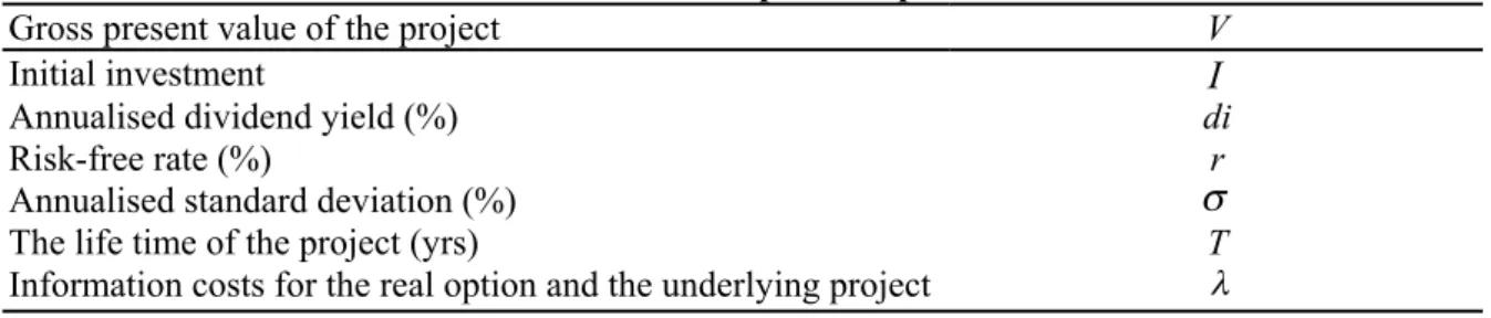
Table 2: Real options Inputs

Gross present value of the project V

Initial investment

I

Annualised dividend yield (%) di

Risk-free rate (%) r

Annualised standard deviation (%)

σ

The life time of the project (yrs) T

Information costs for the real option and the underlying project λ

18 _{or the lost value in time.}

3.2. The value of the option to invest

The value of the option to invest under incomplete information can be computed using the following equation:

1/2GVVσ2V2 + (r +λV – di)VGV – (r +λC)G = 0

This equation for the value of G(V) must satisfy the following conditions: G(0) = 0, G(V*) = V* – I , GV(V) = 1

The value V* is the price at which it is optimal to invest. At that time, the firm receives the difference V* - I. The solution to the differential equation given in Bellalah (2001) is:

G(V) = aVβ (3) where: β = 1/2 – (r +λV – di)/σ2 + ([(r +λV – di)/σ2 - 1/2] 2 + 2(r +λC)/σ 2 )0.5 V* _{= βI/(β –1) , a = (V}*_{– I)/(V}*β₎

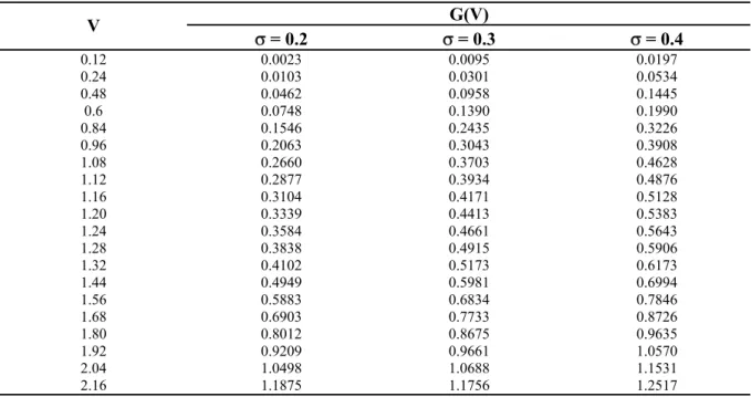
Table 3: Investment opportunity value G(V): the effect of volatility

This Table simulates the value of the investment opportunity G(V), given by equation (3), as a function of the project value, V, in the presence of information costs, λ. r is the interest rate, di is the opportunity cost of delaying project or a constant payout rate, I denotes the cost of investment or investment expenditure, σ stands for the volatility, λC _{(respectively} λV) represents the information cost related to G(V) (respectively V). It is assumed that r = 4 %, δ = 6 %, I = 1, λC = 1 %, and λV = 2 %.

G(V) V σ = 0.2 σ = 0.3 σ = 0.4 0.12 0.0023 0.0095 0.0197 0.24 0.0103 0.0301 0.0534 0.48 0.0462 0.0958 0.1445 0.6 0.0748 0.1390 0.1990 0.84 0.1546 0.2435 0.3226 0.96 0.2063 0.3043 0.3908 1.08 0.2660 0.3703 0.4628 1.12 0.2877 0.3934 0.4876 1.16 0.3104 0.4171 0.5128 1.20 0.3339 0.4413 0.5383 1.24 0.3584 0.4661 0.5643 1.28 0.3838 0.4915 0.5906 1.32 0.4102 0.5173 0.6173 1.44 0.4949 0.5981 0.6994 1.56 0.5883 0.6834 0.7846 1.68 0.6903 0.7733 0.8726 1.80 0.8012 0.8675 0.9635 1.92 0.9209 0.9661 1.0570 2.04 1.0498 1.0688 1.1531 2.16 1.1875 1.1756 1.2517

This Table simulates the value of the investment opportunity, G(V). All things being equal, a larger volatility can be associated with a greater value of the option to invest. And the high project values generate an increase in the value of the option to invest.

3.3. The value of the option to defer

Some projects could increase in value when new information is available and uncertainty decreased with more favourable conditions. The value of waiting to invest or the option to defer can be seen as an American call option on the gross present value of the future expected cash flows.20

The option to defer is reversible and more valuable when there is high economic uncertainty and long investment horizons.21 _{For simplicity, the value of this option can be simulated using the following}

formula.

(

)

(

( )( )

_{( )}

( )

(

(

)

)

)

1 1

, , , ,

, , ,

c S T t c r S c

G V I r di T t

−

σ λ λ

=

η

Ve

−λ λ− −

N

η

_d

−

Ie

−λ+

N

η

_d

−

σ

T t

−

(4) 20 _{Trigeorgis (1996).} 21 _{Ingersoll and Ross (1992).}

With:

(

1 2

)

(

)

2 1 S V Ln r di T t I T t d λ σ σ   + + − + −     = −

Where η=1 for a call and –1 for a put. 3.4. The value of the time-to-build option

Few investments in practice are a single up-front outlay. However, most investments are sequential and staged into several investments. This creates valuable options to default at any given stage. The completion of one stage gives the right but not the obligation to undertake the next stage and the options that this stage provides. The staged investment can be viewed as a series of compound options. In this case, the valuation process can be computed discretely. The project in this case is a perpetual cash flow with a fixed capital outlay. There are points when the project has a positive NPV, but we are better off not taking it because the option to undertake the project in the future is more valuable. Since the investment is irreversible, when we take the project, we destroy the value of waiting. It is possible in this context to extend the standard binomial model to account for the effects of information costs. When generating the binomial tree for the underlying asset, we must account for the information cost of the asset. When we work backward, we must account for the information cost regarding the option.

The valuation procedure in a discrete-time setting in the presence of information costs:

The valuation procedure modifies slightly the binomial model to account for the effects of incomplete information. It can be described in the following steps.

a. The gross present value is V

b. The up multiplier (u) and down multiplier (d) are calculated by using formulas in Cox, Ross and Rubinstein (1979): h e u= σ ,_{d =e}−σ h with: N t T h= − (5) They are used to calculate the future gross value (V) in the nodes of the binomial tree.

c. The risk neutral probability for the up and down branches are calculated as: ( ) d u d e p r d sh − − = − +λ (6) d. The discount factor at each node is:

e

−(r+λc)h ₍₇₎

e. The binomial tree should be constructed in such way that it can incorporate the investments needed. f. Count backward from the end, in every node calculate the value by using the binomial formula for one period and subtracting the value of the investment. To consider this in the binomial tree, the value at each node should be the maximum of the value of the project in the node and zero.

g. The calculation of the value in each node should continue in this backward calculation until the value of the firm finally reaches the present time.

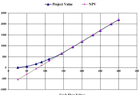
The following Tables 4 and 5 and Figures 1, 2 and 3 simulate the values of the time to build option in the presence of information costs for the option and its underlying asset.

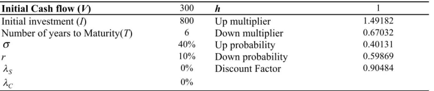
Table 4: Time to build option using binomial approach

Initial Cash flow (V) 300 h 1

Initial investment (I) 800 Up multiplier 1.49182 Number of years to Maturity(T) 6 Down multiplier 0.67032

σ

40% Up probability 0.40131 r 10% Down probability 0.59869 S λ 0% Discount Factor 0.90484 C λ 0%

Figure 1: Time to build binomial tree 3306.95 32269.5 2216.72 21367.2 19333.8 1485.91 21367.2 1485.91 14059.1 14059.1 12721.2 996.035 14059.1 996.035 9160.35 9160.35 8288.63 8288.63 667.662 9160.35 667.662 9160.35 667.662 5876.62 5876.62 5876.62 5317.39 5317.39 447.547 5876.62 447.547 5876.62 447.547 3675.47 3675.47 3675.47 3325.71 3325.71 3325.71 300 3675.47 300 3675.47 300 3675.47 300 2200 2200 2200 2200 1990.64 1990.64 1990.64 2200 201.096 2200 201.096 2200 201.096 1210.96 1210.96 1210.96 1101.45 1095.72 1095.72 1210.96 134.799 1210.96 134.799 1210.96 134.799 547.987 547.987 547.987 558.558 495.839 558.558 90.3583 547.987 90.3583 103.583 103.583 219.362 93.7254 219.362 60.569 103.583 60.569 -194.31 -194.31 37.6132 37.6132 40.6006 -393.99 0 0 27.2154 -527.85

Terminal column has two elements in each state:

•State variable

•NPV

Earlier columns have four elements in each state:

•State variable

•NPV (if project is undertaken)

•Option Value

•Project Value

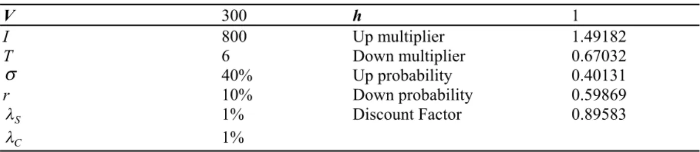
Table 5: Time to build option using binomial approach

V 300 h 1 I 800 Up multiplier 1.49182 T 6 Down multiplier 0.67032

σ

40% Up probability 0.40131 r 10% Down probability 0.59869 S λ 1% Discount Factor 0.89583 C λ 1%

Figure 2: Time to build binomial price and standard NPV -1000 -500 0 500 1000 1500 2000 2500 0 50 100 150 200 250 300 350

Cash Flow Values Project Value NPV

Figure 3: Time to build binomial price and standard NPV

3511.44 34314.4 2353.79 22737.9 20369.4 1577.79 22737.9 1577.79 14977.9 14977.9 13417.7 1057.63 14977.9 1057.63 9776.26 9776.26 8757.91 8757.91 708.948 9776.26 708.948 9776.26 708.948 6289.48 6289.48 6289.48 5634.33 5634.33 475.222 6289.48 475.222 6289.48 475.222 3952.22 3952.22 3952.22 3540.54 3540.54 3540.54 318.551 3952.22 318.551 3952.22 318.551 3952.22 318.551 2385.51 2385.51 2385.51 2385.51 2137.02 2137.02 2137.02 2385.51 213.531 2385.51 213.531 2385.51 213.531 1335.31 1335.31 1335.31 1196.22 1196.22 1196.22 1335.31 143.134 1335.31 143.134 1335.31 143.134 631.342 631.342 631.342 618.278 565.577 631.342 95.9457 631.342 95.9457 159.457 159.457 257.719 142.847 257.719 64.3143 159.457 64.3143 -156.86 -156.86 57.3263 57.3263 43.1112 -368.89 0 0 28.8983 -511.02

3.5. The value of the option to expand

An option to expand is a call option to acquire an additional part to the initial project where the cost to expand is the exercise price. This managerial flexibility has a value and the cost of expanding could be reduced if flexibility is built into the project at an early stage. The value of this option in the presence of shadow costs of incomplete information can be computed using the following formula.

(

)

(

( )( )

_{( )}

( )

(

(

)

)

)

1 1

, , , ,

, , ,

c S T t c r S c

G V I r di T t

−

σ λ λ

=

η

Ve

−λ λ− −

N

η

_d

−

Ie

−λ+

N

η

_d

−

σ

T t

−

(8) With:

(

1 2

)

(

)

2 1 S V Ln r di T t I T t d λ σ σ   + + − + −     = −

Table 6: Time to expand option values using binomial approach

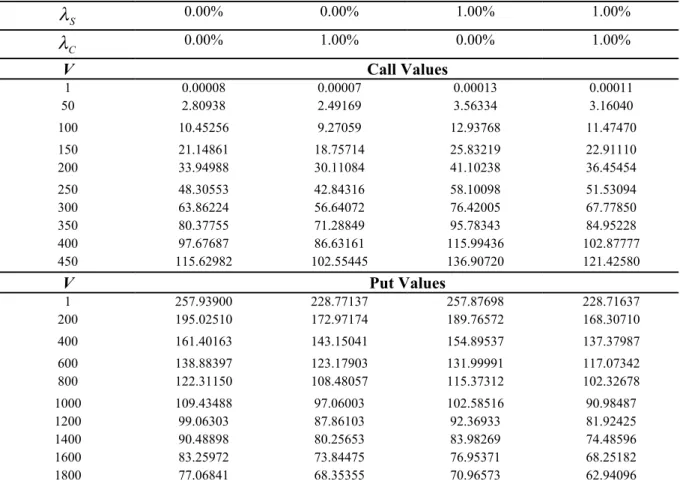
This Table simulates the value of the time to expand option in the presence of information costs for the option and its underlying asset. The valuesofcallsandputsarepresentedtochecktheputcallparityrelationships.ItisassumedthatI = 500,di = 6%,r = 5.5%,σ= 45%, and T = 12.

S

λ

0.00% 0.00% 1.00% 1.00% C

λ

0.00% 1.00% 0.00% 1.00% V Call Values 1 0.00008 0.00007 0.00013 0.00011 50 2.80938 2.49169 3.56334 3.16040 100 10.45256 9.27059 12.93768 11.47470 150 21.14861 18.75714 25.83219 22.91110 200 33.94988 30.11084 41.10238 36.45454 250 48.30553 42.84316 58.10098 51.53094 300 63.86224 56.64072 76.42005 67.77850 350 80.37755 71.28849 95.78343 84.95228 400 97.67687 86.63161 115.99436 102.87777 450 115.62982 102.55445 136.90720 121.42580 V Put Values 1 257.93900 228.77137 257.87698 228.71637 200 195.02510 172.97174 189.76572 168.30710 400 161.40163 143.15041 154.89537 137.37987 600 138.88397 123.17903 131.99991 117.07342 800 122.31150 108.48057 115.37312 102.32678 1000 109.43488 97.06003 102.58516 90.98487 1200 99.06303 87.86103 92.36933 81.92425 1400 90.48898 80.25653 83.98269 74.48596 1600 83.25972 73.84475 76.95371 68.25182 1800 77.06841 68.35355 70.96573 62.94096

This Table simulates the value of the time to expand option in the presence of information costs for the option and its underlying asset. The high project values generate an increase in the value of the option to expand. In the presence of the shadow costs of incomplete information regarding project value, the option value increases. In the case where information costs concern the option value, option to expand value drops instead of increasing. It is of interest to note that the negative effect due to incomplete option value information and the positive effect due to incomplete project value information are compensated. But, on the whole, the presence of two types of information costs increases the option to expand value compared to its level in the complete information case.

3.6. The value of the option to contract

The option to contract has a positive value if market conditions turn weaker than originally expected in this case, management can then reduce the scale of operations and thus saving part of the planned investment outlays. This analogous to a put option on part of the initial project, with exercise price equal

to the potential cost savings. This may be particularly valuable in the case of new-product introductions in uncertain markets.

(

)

(

( )( )

_{( )}

( )

(

(

)

)

)

1 1

, , , ,

, , ,

c S T t c r S c

G V I r di T t

−

σ λ λ

=

η

Ve

−λ λ− −

N

η

_d

−

Ie

−λ+

N

η

_d

−

σ

T t

−

(9) with:

(

1 2

)

(

)

2 1 S V Ln r di T t I T t d λ σ σ   + + − + −     = −

Table 7: Option to contract values

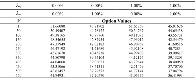
This Table simulates the value of the option to contract in the presence of information costs for the option and its underlying asset. The opportunity to contract the scale of the project by 5%, saving an amount of 100. It is assumed that di = 6%, r = 5.5%, σ= 45%, and T = 12.

S

λ

0.00% 0.00% 1.00% 1.00% C

λ

0.00% 1.00% 0.00% 1.00% V Option Values 1 51.66080 45.81902 51.65769 45.81626 50 50.49407 44.78422 50.34767 44.65438 100 49.38165 43.79760 49.11073 43.55731 150 48.34655 42.87954 47.96912 42.54479 200 47.37949 42.02183 46.90969 41.60516 250 46.47192 41.21689 45.92108 40.72834 300 45.61670 40.45838 44.99408 39.90617 350 44.80790 39.74104 44.12124 39.13203 400 44.04060 39.06051 43.29644 38.40050 450 43.31066 38.41311 42.51459 37.70706 500 42.61457 37.79573 41.77144 37.04794 550 41.94931 37.20570 41.06335 36.41993

This Table simulates the value of the option to contract in the presence of information costs for the option and its underlying asset. As expected, The high project values generate a decrease in the value of the option to contract : the option to contract has a positive value if market conditions are unfavourable. 3.7. The value of the option to shut down and restart operations

The managerial flexibility to be able to shut-down and restart operations can be valuable if prices are such that cash revenues are not sufficient to cover variable operating costs. It might be better not to operate temporarily. If prices rise sufficiently, operations can be restarted. Thus, operations in each year may be seen as a call option to acquire that year’s cash revenues by paying the variable costs of operating as a strike price. It is equivalent to the firm having a portfolio of call and put options. For example, being able to temporarily shut down a project is equivalent to a put option and restarting operations when the project has been down is equivalent to a call option.

Why a company may choose to stay in a line of business (or stay in business, generally, even though it is currently running a loss and the NPV of future operations is negative. The intuition is that there are irreversible costs of exiting and re-entering, and if you exit now, you may wish in the future that you had not.

3.8. The value of the option to abandon

The option to abandon can be valued as an American put option on the project’s current value, with an exercise price corresponding to the salvage or best alternative use value. If prices suffer a sustainable decline or the operation does poorly for some other reason, management may have a valuable option to abandon the project in exchange for its salvage value. The option to abandon a project provides partial insurance against failure.

(

)

(

( )( )

_{( )}

( )

(

(

)

)

)

1 1

, , , ,

, , ,

c S T t c r S c

G V I r di T t

−

σ λ λ

=

η

Ve

−λ λ− −

N

η

_d

−

Ie

−λ+

N

η

_d

−

σ

T t

−

(10) With:

(

1 2

)

(

)

2 1 S V Ln r di T t I T t d λ σ σ   + − + + −     = −

Table 8: Option to abandon values

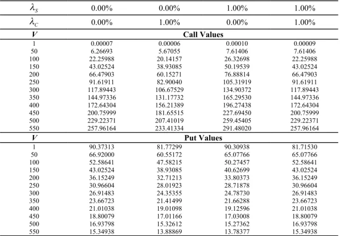
This Table simulates the values of the option to abandon for different levels of information costs. I is the value received on abandonment and T is the number of years until abandon (yrs). It is assumed that I = 150, di = 5%, r = 5%, σ= 40%, and T = 10.

S

λ

0.00% 0.00% 1.00% 1.00% C

λ

0.00% 1.00% 0.00% 1.00% V Call Values 1 0.00007 0.00006 0.00010 0.00009 50 6.26693 5.67055 7.61406 7.61406 100 22.25988 20.14157 26.32698 22.25988 150 43.02524 38.93085 50.19539 43.02524 200 66.47903 60.15271 76.88814 66.47903 250 91.61911 82.90040 105.31919 91.61911 300 117.89443 106.67529 134.90372 117.89443 350 144.97336 131.17732 165.29530 144.97336 400 172.64304 156.21389 196.27438 172.64304 450 200.75999 181.65515 227.69450 200.75999 500 229.22371 207.41019 259.45405 229.22371 550 257.96164 233.41334 291.48020 257.96164 V Put Values 1 90.37313 81.77299 90.30938 81.71530 50 66.92000 60.55172 65.07766 65.07766 100 52.58641 47.58215 50.27457 52.58641 150 43.02524 38.93085 40.62699 43.02524 200 36.15249 32.71213 33.80373 36.15249 250 30.96604 28.01923 28.71878 30.96604 300 26.91483 24.35355 24.78730 26.91483 350 23.66723 21.41499 21.66288 23.66723 400 21.01038 19.01098 19.12596 21.01038 450 18.80079 17.01166 17.03008 18.80079 500 16.93798 15.32612 15.27362 16.93798 550 15.34938 13.88869 13.78377 15.34938

This Table simulates the values of the option to abandon for different levels of information costs and shows that the value of the option to abandon the project increases when market conditions decline severely (that is, when the value of the project is weak).

3.9. The value of the option to switch and the growth option

The firm should be willing to pay a certain positive premium for a flexible technology that can change the inputs from expensive to cheap and change the output from cheap to expensive, depending on the market. Process flexibility can be achieved not only via technology (e.g. by building a flexible facility that can switch among alternative energy inputs), but also by maintaining relationships with a variety of suppliers and switching among them as their relative prices change.

The growth option provides the company with a possibility to make a follow-on investment in the future, it is analogous to a call option. The option to grow is used when an initial investment is required for further development. The project can be considered as a link in a chain of related projects and may serve as a springboard for future project generations. But unless the firm makes that initial investment, subsequent generations will not be feasible.

Kester (1984) recognised the importance of the real growth option on firms and argued that the growth option constituted can account for more than half of the market value for most of the companies. The value of the growth option can be computed using the following formula.

(

)

(

( )( )

_{( )}

( )

(

(

)

)

)

1 1

, , , ,

, , ,

c S T t c r S c

G V I r di T t

−

σ λ λ

=

η

Ve

−λ λ− −

N

η

_d

−

Ie

−λ+

N

η

_d

−

σ

T t

−

(11) with:

(

1 2

)

(

)

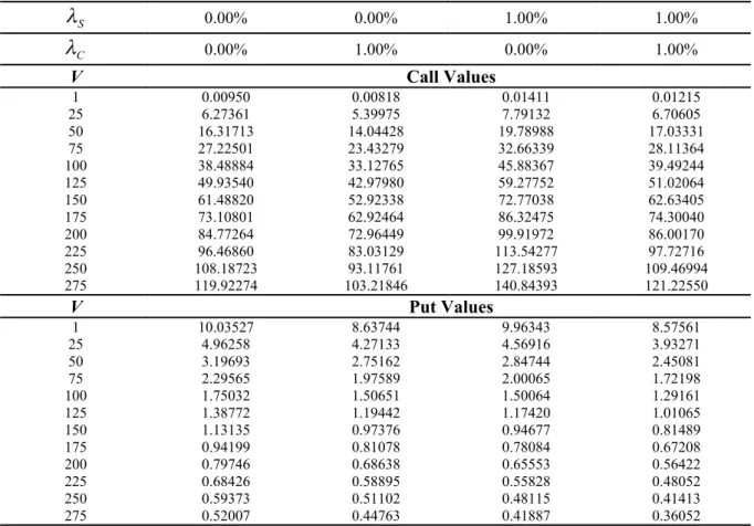
2 1 S V Ln r di T t I T t d λ σ σ   + + − + −     = −

Table 9: Growth option prices

This Table simulates the values of the growth option for different levels of information costs. I is the investment cost. It is assumed that I = 30,

di = 5%, r = 7%, and σ = 35%. S

λ

0.00% 0.00% 1.00% 1.00% C

λ

0.00% 1.00% 0.00% 1.00% V Call Values 1 0.00950 0.00818 0.01411 0.01215 25 6.27361 5.39975 7.79132 6.70605 50 16.31713 14.04428 19.78988 17.03331 75 27.22501 23.43279 32.66339 28.11364 100 38.48884 33.12765 45.88367 39.49244 125 49.93540 42.97980 59.27752 51.02064 150 61.48820 52.92338 72.77038 62.63405 175 73.10801 62.92464 86.32475 74.30040 200 84.77264 72.96449 99.91972 86.00170 225 96.46860 83.03129 113.54277 97.72716 250 108.18723 93.11761 127.18593 109.46994 275 119.92274 103.21846 140.84393 121.22550 V Put Values 1 10.03527 8.63744 9.96343 8.57561 25 4.96258 4.27133 4.56916 3.93271 50 3.19693 2.75162 2.84744 2.45081 75 2.29565 1.97589 2.00065 1.72198 100 1.75032 1.50651 1.50064 1.29161 125 1.38772 1.19442 1.17420 1.01065 150 1.13135 0.97376 0.94677 0.81489 175 0.94199 0.81078 0.78084 0.67208 200 0.79746 0.68638 0.65553 0.56422 225 0.68426 0.58895 0.55828 0.48052 250 0.59373 0.51102 0.48115 0.41413 275 0.52007 0.44763 0.41887 0.36052

This Table simulates the values of the growth option for different levels of information costs. The high project values generate an increase in the value of the growth option. In the presence of the shadow costs of incomplete information regarding project value, the option value increases. In the case where information costs concern the option value, the growth option value drops instead of increasing. And the presence of two types of information costs increases the growth option value compared to its level in the complete information case.

Concluding Remarks

This paper reviews the main well known concepts in real options and extends the literature for the valuation of real options in the presence of information costs as in Bellalah (1999, 2001). These options are fundamental in the valuation process of investments and capital budgeting. However, they are valued in a standard framework ignoring the role of information costs in investment decisions. Information costs play a central role in the capital budgeting process since managers do not invest in projects they do not know about. When money is engaged in research and development, in project analysis and valuation, it is natural to require a return that accounts for these expenses. Therefore, information costs or shadow costs of incomplete information represent a component of the appropriate discount rate in investment decisions.

We introduce information costs in the spirit of Merton (1987), Bellalah (1990), Bellalah and Jacquillat (1995) and Bellalah (1999, 2001) in the capital budgeting process and real options valuation. We develop a general derivation for the valuation of options when the underlying asset is observable and when it is not observable. This provides a generalisation of the Black-Scholes (1973) formula and Merton (1998) formula which accounts for the effects of incomplete information. We present different

formulas for the valuation of the option to defer, the time to build option, the option to shut down and restart option, the option to abandon, the switch option and the growth option in the presence of information costs. Simulation results are provided using reasonable values for information costs. Our analysis can be extended to other types of real options. In particular, it can be applied to compound real options and “exotic” real options using the same techniques as those in the pricing of exotic options as shown in Bellalah (2000). The models can also be tested using real data. It is also possible to extend these models to account for stochastic volatility of the cash flows as in Aboura, Bellalah, Villa and Prigent (2000).

REFERENCES

Aboura, S., Bellalah, M., Villa, C. and Prigent, J.L. (2000) "Skew without Skewness", Paper presented at EFMA Conference, Paris, June.

Agmon, T. (1991) “Capital Budgeting and the Utilization of Full Information: Performance Evaluation and the Exercise of Real Options”, Managerial Finance, vol. 17, N. 2/3, 42-50.

Amihud, Y. and Mendelson, H. (1986) "Asset Pricing and the Bid-Ask Spread", Journal of Financial

Economics, 17, 223-249.

Amihud, Y. and Mendelson, H. (1988) "Liquidity and Asset Pricing: Financial Management Implications", Financial Management, spring, 5-15.

Bellalah, M., (1990) "Quatre essais sur l’évaluation des options sur indices et sur contrats à terme d’indice: dividende, volatilité et information incomplète", Thèse de Doctorat, Université de Paris-Dauphine, Juin.

Bellalah, M. and Jacquillat, B. (1995) "Option Valuation with Information Costs: Theory and Tests",

Financial Review, August, 617-635.

Bellalah, M. (1999) "The valuation of futures and commodity options with information costs",

Journal of Futures Markets, September.

Bellalah, M. (2000) "The valuation of exotic and real options: a survey of some important results",

Finance, a special issue, June.

Bellalah, M. (2001) "Irreversibility, Sunk Costs and Investment Under Incomplete Information",

R&D Management.

Berger, P.G., Ofek, E. and Swary, I. (1996) “Investor valuation of the abandonment option” Journal

of Financial Economics, 42, 257-287.

Black, F. and Scholes, M. (1973) “The Pricing of Options and Corporate Liabilities”, Journal of

Political Economy, N. 81, 673-659.

Brealey, R.A. and Myers, S.C. (1985) “Principles of Corporate Finance”, third edition. McGraw-Hill.

Brennan, M. and Cao, H. (1997) “International Portfolio investment flows”, Journal of Finance, Vol. LII, N. 5, December, 1851-1879.

Brennan, M.J. and Schwartz, E. (1985) “Evaluating natural resource investments”, Journal of

Business.

Copeland, T. and Weston, F. (1988) “Financial Theory and Corporate Policy”, Addison Wesley, NY. Coval, J. and Moskowitz, T. F. (1999) "Home bias at home: local equity preference in domestic portfolios", Working Paper, University of Michigan.

Cox, J.C. and Ross, S.A. and Rubinstein, M. (1979) “Option pricing: A simplified approach”,

Journal of Financial Economics, 7, N. 3, 229-263.

Cox, J.C. and Ross, S.A. (1976) “A Survey of Some New Results in Financial Option Pricing Theory”, The Journal of Finance, XXXI, N. 2, May.

Cox, J. C. and Rubinstein, M. (1985) “Options Markets”, Prentice-Hall.

Dentskevich, P. and Salkin, G. (1991) “Valuation of Real Projects Using Option Pricing Techniques”, OMEGA International Journal of Management Science, Vol. 19, N. 4, 207-222.

Dixit, A.K. (1992) “Investment and Hysteresis”, Journal of Economic Perspectives, vol. 6, N. 1, winter, 107-132.

Dixit, A.K. (1995) “Irreversible investment with uncertainty and scale economies”, Journal of

Economic Dynamics and Control, N. 19, 327-350.

Dixit, A.K. and Pindyck, R.S. (1993) “Investment under uncertainty”, Princeton, NJ.

Dixit, A.K. and Pindyck, R.S. (1995) “The Options Approach to Capital Investment”, Harvard

Business Review, May-June, 105-115.

Dixit, A., Pindyck, R.S. and Sodal, S. (1999) “A Markup Interpretation of Optimal Investment Rules”, Economic Journal, Vol. 109, N. 455, April, 179-189.

Edwards, M. and Wagner, H. (1999) "Capturing the research advantage", Journal of Portfolio

Management, Spring, 18-24.

Faulkner, T.W. (1996) “Applying ‘Options Thinking’ To R&D Valuation”, Research and

Technology Management, May-June.

Foerster, S. and Karolyi, G. (1999) "The effect of market Segmentation and investor recognition on Asset Prices: evidence from foreign stocks listing in the United States", Journal of Finance, 49,981-1014.

Ingersoll, J.E. and Ross, S.A. (1992) “Waiting to Invest: Investment and Uncertainty”, Journal of

Business, Vol. 65, N. I, 1-30.

Kadlec, G. and McConnell, J. (1994) "The effect of market Segmentation and Illiquidity on Asset Prices: evidence from Exchange Listings", Journal of Finance, 49, 611-635.

Kang, J. and Stulz, R. (1997) "Why is there a home bias? an analysis of foreign portfolio equity in Japan", Journal of Financial Economics, 46, 3-28.

Kester, W.C. (1984) “Today’s options for tomorrow’s growth”, Harvard Business Review, March-April, 153-160.

Kester, W.C. (1993) “Turning Growth Options into Real Assets”, Capital budgeting under

uncertainty, 187-207.

Kogut, B. (1991) “Joint Ventures and the Option to Expand and Acquire”, Management Science, Vol. 37, N. 1, January.

Kogut, B. and Kulatilaka, N. (1994a) “Operating Flexibility, Global Manufacturing, and the Option Value of a Multinational Network”, Management Science, Vol. 40, N. 1, January.

Kogut, B. and Kulatilaka, N. (1994b) “Options Thinking and Platform Investments: Investing in Opportunity”, California Management Review, Vol. 36, N. 2, winter.

Kulatilaka, N. (1993) “The Value of Flexibility: The Case of a Dual-Fuel Industrial Steam Boiler”,

Financial Management, Vol. 22, N. 3, Autumn, 271-280.

Lee, C.J. (1988) “Capital Budgeting under Uncertainty: The Issue of Optimal Timing”, Journal of

Business Finance and Accounting, 15(2) Summer.

McDonald, R. and Siegel, D. (1984) “Option pricing when the underlying assets earns a below-equilibrium rate of return: a note”, Journal of Finance.

McDonald, R. and Siegel, D. (1986) “The value of waiting to invest”, Quarterly Journal of

Economics.

Merton, R. (1987) "A Simple Model of Capital Market Equilibrium with Incomplete Information",

Journal of Finance, Vol. 42, N. 3, July, 483-510.

Merton, R.C. (1998) “Applications of option pricing theory: twenty five years later”, American

Economic Review, Vol. 88, N. 3, 323-345.

Myers, S. C. (1977) “Determinants of Corporate Borrowing”, Journal of Financial Economics, Volume 5, N. 2, November, 147-175.

Myers, S.C. (1984) “Finance Theory and Financial Strategy” Interfaces, 14:1, Jan.-Feb., 126-137. Myers, S.C. and Majd, S. (1990) “Abandonment Value and Project Life”, Advances in Futures and

Options Research, Vol.4, 1-21.

Newton, D. (1996) “Opting for the right value for R&D”, The Financial Times, June, 28.

Paddock, J., Siegel, D. and Smith, J. (1988) “Option valuation of claims on real assets: the case of offshore petroleum leases”, Quarterly Journal of Economics.

Pindyck, R.S. (1991) “Irreversibility, Uncertainty, and Investment”, Journal of Economic Literature, Vol. XXIX, Sept., 1100-1148.

Siegel, D.J., Smith, and Paddock, J. (1987) “Valuing offshore oil properties with option pricing models”, Midland Corporate Finance Journal.

Smith, J.E. and Nau, R.F. (1994) “Valuing Risky Projects: Option Pricing Theory and Decision Analysis”, Management Science, Vol. 41, N. 5, May.

Stulz, R. (1999) "Globalization of equity markets and the cost of capital", Working Paper, February, 923-934.

Trigeorgis, L. (1990) “A Real Option Application in Natural-Resource Investments”, Advances in

Futures and Options Research, Vol. 4, 153-156.

Trigeorgis, L. (1993) “The Nature of Options Interactions and the Valuation of Investments with Multiple Real Options”, Journal of Financial and Quantitative Analysis, Vol. 28, N. 1, March, 1-20.

Trigeorgis, L. (1993) “Real Options in Capital Investments, models, strategies, and applications”, Praeger Publishers, Westport.

Trigeorgis, L. (1996) “Real Options - Managerial Flexibility and Strategy in Resource Allocation”, The MIT Press.