HAL Id: tel-02299759
https://pastel.archives-ouvertes.fr/tel-02299759v2
Submitted on 2 Feb 2020HAL is a multi-disciplinary open access archive for the deposit and dissemination of sci-entific research documents, whether they are pub-lished or not. The documents may come from teaching and research institutions in France or abroad, or from public or private research centers.
L’archive ouverte pluridisciplinaire HAL, est destinée au dépôt et à la diffusion de documents scientifiques de niveau recherche, publiés ou non, émanant des établissements d’enseignement et de recherche français ou étrangers, des laboratoires publics ou privés.
tissues
Lamiae Abdeladim
To cite this version:
Lamiae Abdeladim. Large volume multicolor nonlinear microscopy of neural tissues. Optics [physics.optics]. Université Paris Saclay (COmUE), 2018. English. �NNT : 2018SACLX070�. �tel-02299759v2�
Th
`ese
de
doctor
at
NNT
:
2018SA
CLX070
microscopy of neural tissues
Th `ese de doctorat de l’Universit ´e Paris-Saclay pr ´epar ´ee `a l’Ecole Polytechnique Ecole doctorale n◦573 interfaces : approches interdisciplinaires, fondements, applications et innovation (INTERFACES) Sp ´ecialit ´e de doctorat : Physique
Th `ese pr ´esent ´ee et soutenue `a Palaiseau, le 27/09/2018, par
M
ME
L
AMIAE
A
BDELADIM
Composition du Jury :
Dr. Philippe Vernier
Directeur de recherche, CNRS Pr ´esident
Dr. Laurent Bourdieu
Directeur de recherche, CNRS Rapporteur
Dr. Martin Oheim
Directeur de recherche, CNRS Rapporteur
Dr. Rosa Cossart
Directrice de recherche, Inserm Examinatrice
Dr. Emmanuel Beaurepaire
Directeur de recherche, CNRS Directeur de th `ese
Dr. Willy Supatto
Charg ´e de recherche, CNRS Co-directeur de th `ese
Dr. Jean Livet
M
ultiphoton microscopy has transformed neurobiology during the two last decades by en-abling 3D imaging of thick tissues at subcellular resolution. However the depths provided by multiphoton microscopy are limited to few hundreds of micrometers inside scattering tissues such as the brain. In the recent years, several strategies have emerged to overcome this depth limitation and to access larger volumes of tissue. Although these novel approaches are transforming brain imaging, they currently lack efficient multicolor and multicontrast modalities. This work aims to develop large-scale and deep-tissue multiphoton imaging modalities with augmented contrast capabilities. In a first chapter, we present the challenges of high-content large-volume brain imaging, with a particular emphasis on powerful multicolor labeling strategies which have so far been restricted to limited scales. We then introduce chromatic serial multi-photon tomography, a method which combines automated histology with wavelength-mixing to access multiple nonlinear contrasts across large volumes, from several mm3to whole brains, with submicron resolution and intrinsic channel registration. In a third chapter, we demonstrate the potential of this novel approach to open novel experimental paradigms in neurobiological studies. In particular, we demonstrate multicolor volumetric histology of several mm3of Brainbow-labeled tissues with preserved diffraction-limited resolution and illustrate the strengths of this method through color-based tridimensional analysis of astrocyte morphology, interactions and lineage in the mouse cerebral cortex. We further illustrate the potential of the method through multiplexed whole-brain mapping of axonal projections labeled with distinct tracers. Finally, we develop multimodal three-photon microscopy as a method to access larger depths in live settings.Key words: Multiphoton microscopy, wavelength-mixing, block-face imaging, three-photon
A
u moment où je m’apprête à écrire ces fameux remerciements de thèse, je suis en pleine préparation de mon départ, bientôt imminent, de l’autre côté de l’Atlantique. C’est donc non sans nostalgie, mais surtout avec beaucoup de gratitude que je prend ces quelques lignes pour remercier toutes celles et ceux qui ont contribué à cette aventure.Je commencerai tout d’abord par remercier les membres de mon jury: Laurent Bourdieu, Martin Oheim, Rosa Cossart et Philippe Vernier. Merci à chacun et chacune d’avoir pris de votre temps pour évaluer mon travail. Merci pour vos retours constructifs et vos encouragements. Par ailleurs, je remercie doublement Laurent et Martin pour leur travail de rapporteurs. Je tiens ensuite à remercier la direction du LOB, tout d’abord Jean-Louis Martin pour m’avoir accueillie au laboratoire puis particulièrement François Hache pour son suivi ces quatre dernières années, et d’avoir toujours été à l’écoute des doctorants.
J’ai eu beaucoup de chance d’être encadrée par trois chercheurs extraordinaires (et non, je n’exagère rien !). Emmanuel, cette thèse a d’abord été pour moi une fabuleuse rencontre scien-tifique et humaine. Merci infiniment pour ces quatre belles années: you literally changed my life ! Merci pour ta vision, ta générosité, ton soutien sans failles et tout ce que tu m’as transmis. Merci de m’avoir aidée à me construire et à évoluer. Merci pour ton aura positive au quotidien et de réussir à voir le meilleur et à faire ressortir le meilleur en chacun. Merci de m’avoir supportée et soutenue dans les moments difficiles. Je pense qu’on ne peut juste pas rêver d’avoir un meilleur directeur de thèse. Jean, ça a été un énorme plaisir et privilège de travailler avec toi. Merci de m’avoir introduit au merveilleux monde de la neuro (tout en couleurs en plus !). Mais surtout merci de m’avoir très tôt convaincue que je pouvais faire des neurosciences au plus haut niveau malgré mon parcours de physicienne, c’est fondamentalement ce qui m’a donné l’audace de choisir un labo de neurophysiologie pour mon postdoc. Et merci de m’avoir toujours encouragée à voir grand. Willy, merci d’avoir toujours répondu présent quand j’en ai eu besoin. Merci pour toutes les techniques que tu m’as apprises qui ont beaucoup contribué à me construire une culture très large en microscopie et qui me seront certainement précieuses pour la suite. Merci également pour ta précieuse aide Imaris, tes retours toujours pertinents et pour tous tes conseils pour la suite. A tous les trois, je suis fière d’avoir fait ma thèse avec vous, et encore une fois merci pour tout.
J’ai également eu la chance de travailler avec deux jeunes neurobiologistes talentueuses, Katie Matho et Solène Clavreul, que je tiens à remercier pour tout leur travail et les beaux projets qu’on a pu réaliser ensemble. Ca a été un vrai plaisir de travailler avec vous, et j’espère que l’occasion se renouvellera par la suite ! Katie, merci pour tout ce que tu m’as appris et d’être toujours là pour partager ton expérience. On viendra à bout de ce projet titanesque ! Solène, tu m’as inspirée par ta rigueur et ta détermination, j’ai hâte de voir la suite ! J’en profite également pour remercier les autres collaborateurs ayant contribué à ce travail de thèse: Khmaies Guesmi
Sébastien Février et Patrick Cadroas pour les tout premiers essais 3P.
Vient ensuite le tour des Lobsters avec qui j’ai eu l’occasion de travailler. Tout d’abord, un énorme merci à Chiara, pour tous les échanges scientifiques, tes encouragements au quotidien, et tous les bons moments passés au labo et en dehors. I will definitely miss you. Un grand merci également à Pierre d’avoir travaillé avec moi pour upgrader les setups, j’ai énormément appris avec toi ! Merci à Anatole pour ton ouverture d’esprit et tes inputs sur les projets, et merci à Son et à toi d’avoir sublimé le travail MNTB. Merci à Guy, pour avoir été un labmate admirable pendant trois ans, et pour m’avoir fait découvrir la culture israélienne. Un grand merci aussi à Nicolas O. pour toutes les discussions et les précieux conseils, et surtout de m’avoir convaincue de me mettre à LateX pour la rédaction! Je t’en suis éternellement reconnaissante !
Merci également à l’indispensable team technique du LOB. Merci à Laure et Christelle pour votre fantastique efficacité, à Jean-Marc pour ta créativité qui nous aide à réaliser nos designs les plus fous, à Xavier pour les belles conceptions électroniques, et à Isabelle de m’avoir aidée à sécuriser les protocoles que j’ai mis en place. Je n’oublie évidemment pas Emilie et Ernan, pour leur bonne humeur et leur gentillesse !
Je voudrais aussi dire merci à toutes celles et ceux qui m’ont suivie et encouragée ces dernières années, je pense notamment à Laura, Roxane, Adeline, Marie-Claire, Nicolas D., Gaël, Karsten, Hannu, Manuel, et tous les autres que j’aurais oublié.
J’ai biensur une pensée chaleureuse pour mes valeureux compagnons de route, les djeun’s du LOB: Helene, Lipsa, Guillaume, Claire, Chao, Joséphine, Julia, Paul, Antoine, Arthur, Margaux, Mayla, Xiujun, Yoann, Clothilde. Un merci particulier à Julia pour son énergie positive et ses encouragements pendant la rédaction et à Joséphine de m’avoir aidée à relativiser par moments. Un petit clin d’oeil aussi à Max et Pascal parce qu’ils sont juste trop cool (et pour les gateaux du vendredi apm).
Enfin un dernier merci aux lunchmates du dernier départ Magnan: Emmanuel, Chiara, Nicolas, Guy : merci pour ces chouettes moments à refaire le monde, les sciences, la politique, en 30 min chrono!
Je prendrai ces dernières lignes pour remercier mes proches qui ont beaucoup contribué à mon équilibre ces dernières années. Merci à mes amis (pardon d’avance à ceux que j’oublie): Chiara P, Hyacinthe et Aude pour avoir pris soin de moi et pour votre soutien continu et tous les autres pour les bons moments passés ensemble Olivier, François, Elodie, Maxime, Louis, Vincent, Pilou, Madeleine, Anne-Laure, Marie, Nico, Matthieu, Jean, Hélène, Fanny, Elena et le club MPSI2 de Saint-Louis. Je vous attends tous en Californie! Merci à toute la famille Dalens de m’avoir ’adoptée’ et pour tous les chaleureux moments passés ensemble. Merci à mon papa de m’avoir permis de faire des études longues, en France de surcroît. Merci à ma maman de m’avoir toujours encouragée à me battre et à me dépasser. Merci à Sabrine de croire si fort en moi et de m’encourager à aller toujours plus loin. Enfin merci à Théo pour tout le bonheur que tu m’apportes chaque jour, merci de m’aider à réaliser mes rêves et de me rappeler souvent que rien n’est impossible.
Page
List of Tables ix
List of Figures xi
1 Introduction 1
1.1 Imaging the brain: technologies, scales and challenges . . . 1
1.2 Multiphoton microscopy: principles and applications in neurobiology . . . 3
1.2.1 Principles of non-linear excitation . . . 3
1.2.2 Experimental multiphoton microscope systems . . . 5
1.2.3 Sources of contrast . . . 7
1.2.4 Imaging depth in multiphoton microscopy . . . 8
1.2.5 Photodamage . . . 10
1.2.6 Multiphoton microscopy in neurobiology . . . 11
1.3 Multicolor labeling strategies . . . 11
1.3.1 Genetic and molecular tools for fluorescence labeling . . . 12
1.3.2 The Brainbow technology . . . 13
1.3.3 Multicolor strategies for lineage tracing . . . 15
1.3.4 Multicolor strategies for connectivity and neuroanatomical studies . . . 18
1.4 Multicolor multiphoton microscopy . . . 20
1.4.1 Strategies for multicolor nonlinear microscopy . . . 21
1.4.2 Multicolor two-photon microscopy using wavelength-mixing . . . 22
1.5 Challenges and aims . . . 24
2 Chrom-SMP: Principles and Implementation 27 2.1 Block-face and microtome-assisted large volume light microscopy approaches: state of the art . . . 27
2.1.1 Initial efforts . . . 28
2.1.2 Wide-field approaches: MOST, fMOST and WVT . . . 29
2.1.3 Serial two-photon tomography (STP) and derived methods . . . 31
2.1.5 Chrom-SMP: rationale . . . 33
2.2 Chrom-SMP: experimental setup and performances . . . 34
2.2.1 Experimental setup . . . 34
2.2.2 Tissue processing . . . 39
2.2.3 Tissue sectioning . . . 43
2.2.4 Optical performances . . . 45
2.3 Chrom-SMP: Image processing workflow . . . 47
2.3.1 Individual tile processing . . . 48
2.3.2 Dataset stitching . . . 50
2.3.3 Color processing . . . 51
2.4 Chrom-SMP validation: whole-brain serial multicolor tomography . . . 53
2.5 Multimodal brain-wide imaging using Chrom-SMP . . . 54
2.5.1 Coherent contrasts . . . 54
2.5.2 Multimodal brain-wide imaging using Chrom-SMP . . . 58
2.6 Conclusion and perspectives . . . 62
3 Chrom-SMP: applications in neurobiology 67 3.1 Multicolor volumetric histology . . . 67
3.1.1 Multicolor semi-sparse cortical astrocytes labeling . . . 68
3.1.2 Continuous high-resolution multicolor imaging over several mm3volumes of mouse cerebral cortex . . . 70
3.1.3 Dense astroglial network reconstruction . . . 73
3.1.4 Individual astrocyte volumes across cortical layers . . . 75
3.1.5 3D reconstructions of astrocyte-astrocyte contact . . . 78
3.2 Large volume clonal analysis . . . 83
3.2.1 Multicolor astrocyte clonal labeling . . . 83
3.2.2 3D large volume clonal datasets . . . 84
3.3 Whole-brain multiplexed projection mapping . . . 85
3.3.1 STP tomography-based mesoscale connectomics . . . 86
3.3.2 Multiplexed projection mapping with Chrom-SMP . . . 87
3.4 Conclusion and perspectives . . . 97
4 Multi-contrast deep-tissue three-photon microscopy 101 4.1 Strategies for deep-tissue multiphoton imaging . . . 102
4.1.1 Strategies for deep-tissue imaging . . . 102
4.1.2 Three-photon microscopy for deep-tissue imaging . . . 104
4.1.3 Three-photon microscopy: state of the art . . . 108
4.2 SWIR laser sources for three-photon microscopy . . . 110
4.2.2 SWIR laser sources for 3P microscopy : state of the art . . . 112
4.2.3 Comparison of two custom-built SWIR sources for red 3PEF . . . 114
4.3 Dual-color three-photon microscopy . . . 120
4.3.1 OPCPA source design . . . 121
4.3.2 Experimental setup and validation . . . 122
4.3.3 Multimodal three-photon imaging in scattering tissues . . . 124
4.3.4 Live dual-color 3P microscopy . . . 127
4.4 Conclusion and perspectives . . . 129
5 General conclusion 133
TABLE Page
1.1 Multicolor strategies for lineage and clonal analysis. . . 25
2.1 Acquisition parameters in Chrom-SMP experiments. . . 38
2.2 Vibratome settings for regular and soft tissue sectioning. . . 43
4.1 Orders of magnitude of nPEF action cross sections. . . 110
FIGURE Page
1.1 Brain size scales . . . 2
1.2 Methods for brain imaging . . . 2
1.3 1PEF Vs. 2PEF . . . 3
1.4 Optical sectioning . . . 4
1.5 Scanning strategies . . . 5
1.6 Point-scanning multiphoton microscope . . . 6
1.7 Modes of contrast in multiphoton microscopy . . . 7
1.8 Absorption coefficients. . . 8
1.9 Scattering in biological tissues . . . 9
1.10 Light-induced toxicity mechanisms in multiphoton microscopy. . . 10
1.11 The Brainbow strategy . . . 14
1.12 Principle of multicolor lineage analysis with Brainbow. . . 16
1.13 The MAGIC marker strategy . . . 17
1.14 Radially oriented streams of clonally related cells in chick embryonic tissues . . . 17
1.15 Nucbow/Cytbow . . . 18
1.16 Applications of Brainbow to neuroanatomy . . . 20
1.17 Multicolor nonlinear strategies . . . 21
1.18 Multicolor 2P microscopy using wavelength-mixing . . . 23
2.1 Wide-field automated sectioning techniques . . . 30
2.2 Serial two-photon tomography (STP). . . 31
2.3 Color contrast in automated histology methods. . . 33
2.4 Chrom-SMP setup . . . 34 2.5 Wavelength-mixing stage . . . 35 2.6 Scan system . . . 36 2.7 Sample stage . . . 37 2.8 Detection stage . . . 39 2.9 Integration-based detection . . . 40
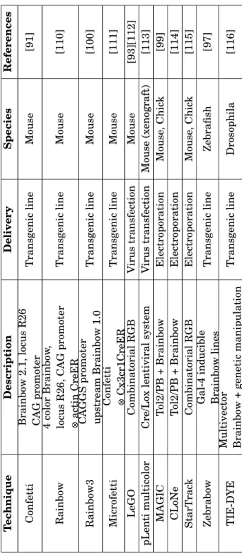
2.11 Vibratome striae. . . 43
2.12 Influence of cross-linking on slicing quality. . . 44
2.13 Lossless imaging with Chrom-SMP . . . 44
2.14 Lateral and axial point-spread function (PSF) matching . . . 45
2.15 Chromatic aberration . . . 46
2.16 Multicolor voxel precision . . . 48
2.17 Visualization and processing workflow . . . 49
2.18 Flat-field correction profiles . . . 49
2.19 Flat-field correction . . . 50
2.20 Unmixing ternary plots . . . 51
2.21 Unmixing polar plots . . . 52
2.22 Unmixing Brainbow dataset . . . 53
2.23 Whole-brain multicolor serial tomography . . . 54
2.24 High-resolution multicolor anatomical views acquired with Chrom-SMP. . . 55
2.25 THG nonlinear process . . . 56
2.26 THG contrast . . . 57
2.27 Nonlinear processes in CARS signal . . . 57
2.28 CARS contrast . . . 58
2.29 Brain-wide label-free THG/CARS imaging . . . 59
2.30 THG contrast in mouse brain tissue . . . 60
2.31 CARS contrast in mouse brain tissue . . . 61
2.32 THG vs. CARS . . . 62
3.1 Protoplasmic astrocyte morphology . . . 69
3.2 Sequence of development of neurons and glial cell in the mouse brain . . . 70
3.3 Continuous 3D hig-resolution multicolor imaging of mouse cortical tissue . . . 71
3.4 3D stitching . . . 72
3.5 Multicolor large volume imaging with multicolor voxel precision . . . 72
3.6 Astrocyte domains . . . 73
3.7 Astrocyte 3D positions . . . 74
3.8 Example of detected color combinations . . . 74
3.9 Reconstruction of labeled astrocytes and their environmet . . . 75
3.10 Methodology for 3D astrocyte volume analysis . . . 76
3.11 Volume of astrocyte domains . . . 77
3.12 Dense Brainbow astrocyte labeling . . . 79
3.13 Morphological analysis of astrocyte-astrocyte contacts . . . 79
3.14 Interface 3D reconstruction workflow . . . 81
3.15 Astrocyte-astrocyte contact analysis . . . 82
3.17 Large volume multicolor clonal analysis with Chrom-SMP . . . 84
3.18 Cortical astrocyte clones at different developmental stages . . . 85
3.19 Volume of cortical astrocytes at two developmental stages . . . 86
3.20 Analysis of the 3D spatial arrangements of astrocyte clones . . . 86
3.21 Mesoscale connectomics . . . 87
3.22 Brain-wide multiplexed projection mapping with Chrom-SMP . . . 89
3.23 Triple AAV injection . . . 89
3.24 Projection mapping across the forebrain . . . 90
3.25 3D topography patterns . . . 91
3.26 Neural projection dissection with Chrom-SMP . . . 92
3.27 Quantitative projection analysis workflow . . . 92
3.28 Linear unmixing procedure . . . 92
3.29 Multithreshold clustering . . . 93
3.30 Automated contrast enhancement . . . 94
3.31 Segmentation algorithm layout . . . 94
3.32 Signal segmentation . . . 95
3.33 Projection strength maps . . . 96
3.34 Interdigitation maps . . . 96
3.35 Brain-wide multicolor AAV/THG imaging . . . 97
4.1 Depth limitation in two-photon microscopy. . . 104
4.2 Absorption and scattering in the near-infrared range. . . 105
4.3 Excitation confinement in 2PEF and 3PEF. . . 106
4.4 Three-photon microscopy in the SWIR range: state of the art. . . 109
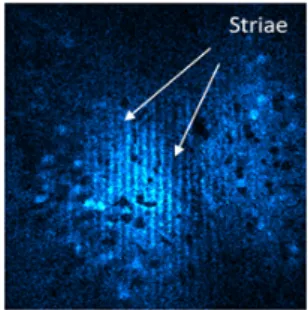
4.5 Signal vs. duty cycle. . . 111
4.6 Experimental setup for 3P microscopy at 1700 nm. . . 115
4.7 THG/3PEF imaging at 1650 nm with a 50 MHz fiber laser . . . 116
4.8 3PEF/THG imaging in fixed bran tissue with a MHz OPA . . . 117
4.9 Live 3PEF/THG imaging of a developing Drosophila embryo with the 50 MHz fibered source . . . 118
4.10 Live 3PEF/THG imaging of a developing Drosophila embryo displaying red nuclei labeling with the MHz OPA source . . . 119
4.11 Comparison of OPO (80 MHz, 1200 nm) and OPA (1.2 MHz, 1700 nm) THG imaging. 120 4.12 Multiband MHz OPA source general architecture. . . 121
4.13 Multiband MHz OPA source experimental setup. . . 122
4.14 Dual-color three-photon microscopy setup. . . 123
4.15 Axial resolution during two-color 3PEF imaging. . . 124
4.16 Dual-color 3PEF imaging for several combinations of green-red fluorescent proteins. . 125
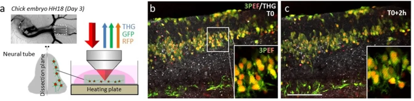
4.18 Deep-tissue imaging of fixed chick spinal tissue . . . 126 4.19 Red and green 3PEF vs. 2PEF contrasts. . . 126 4.20 Multicolor 3PEF 2h time-lapse with dual-compartment red/green labeling. . . 128 4.21 Simultaneous dual-color 3PEF and THG time-lapse imaging of developing chick
embryo spinal cord tissue expressing cytoplasmic red/green labeling . . . 129 4.22 Adult fish telencephalon. . . 130
C
H A P1
I
NTRODUCTION1.1
Imaging the brain: technologies, scales and challenges
Understanding how the brain develops and how it is organized to drive and support all the diversity and complexity of behavioral phenotypes is a major goal of 21stcentury modern neuro-science. From the structural perspective, the challenge raises from the outstandingly complex architecture of the brain : if we take the example of the mouse brain, which is already orders of magnitude smaller than a human brain (Fig 1.1), it contains no less than approximately a hundred of millions of neurons, and almost as many glial cells.
Imaging the brain at the cellular and circuit level poses the following challenges:
(i) Volume: The mouse brain is approximately 0.6 ×0.9 ×1.1 mm3 with neurons projecting axons across several millimeters. Brain areas are also largely heterogeneous and functionnally diverse, so mm3 to cm3volumetric imaging is required to capture cellular ensembles within a network/functional areal scale.
(ii) Resolution: Neurons usually present thin micron/sub-micron axons and dendritic arbors. Glial cells such as astrocytes also present a highly ramified structure with fine cellular processes. Micron-scale resolution is therefore required.
(iii) Contrast/Specificity: Because of the high density and heterogeneity of tightly connected cells in the nervous system, contrast strategies are required to label, visualize and identify individual cells or cell populations of interest within their complex environment.
Fig 1.2 gives an overview of some of the most widely used optical and non optical technologies used for brain imaging. At first glance, one can notice the inevitable trade-off between accessible imaging depth and achievable resolution. Indeed, MRI/fMRI approaches provide whole-organ access, however with a millimetric resolution, not sufficient for cellular/sub-cellular imaging. On the other edge of the spectrum, super-resolution and electron microscopy provide synaptic
FIGURE 1.1. Comparison of brain anatomical scales across three mammalian species. Yellow: mass. Red: number of neurons. Adapted from [4].
FIGURE 1.2. Comparison depth vs. resolution for different imaging methods. MRI:
magnetic resonance imaging.
nanoscale and sub-nanoscale resolution respectively, but within restricted micrometric volumes, although recent outstanding efforts have recently aimed at increasing the accessible volume by harnessing serial tissue sectioning [1][2]. In between these edges, multiphoton microscopy provides cellular to sub-cellular micron-scale resolution upon hundreds of microns of depth within thick tissues, with the additional advantage of providing multiple contrast possibilities [3].
Yet the last five years have witnessed an outburst of technologies aiming to bridge these scales together and overcome the volume/resolution trade-off in light microscopy, both in live (three-photon microscopy using higher wavelengths in the near-infrared [5]) and histological (serial block-face and optical clearing approaches [6][7][8][9]) contexts. Since our starting point in this thesis is multiphoton microscopy, the upcoming section will be devoted to the fundamentals of this technology.
FIGURE1.3. One-photon excited (1PEF) vs. two-photon excited (2PEF) Jablonski dia-grams. Adapted from [16].
1.2
Multiphoton microscopy: principles and applications in
neurobiology
The collective absorption of multiple photons following a high temporal and spatial concentration of photons has been theoretically demonstrated in 1931 by Maria Goeppert Mayer in her doctoral dissertation (english translation available at [10]). However, it was not until the development of the first lasers that the effect could be experimentally validated in the 60s. In 1978, Sheppard and Kompfner conceptualized the principle of a multiphoton scanning microscope [11], but again many years have passed before the first effective experimental implementation of a scanning microscope based on two-photon excited fluorescence by W. Denk, J. Strickler and W. Webb in 1990 [12]. In the early 2000’s, propelled by the development of turn-key femtosecond laser source, several technological developments have contributed to the maturation of the technology [13][14][15]. In the last ten years, multiphoton microscopy hence became an indispensable tool to study live and intact tissues, both to answer fundamental biological questions and also in more biomedical/clinical contexts. In particular, multiphoton microscopy has had a revolutionary impact in 21stcentury modern neuroscience. In this section, we will first briefly review some fundamentals of multiphoton microscopy. In the last paragraph, we will give a very short overview of its use in neurobiology.
1.2.1 Principles of non-linear excitation
In a nonlinear excitation process, multiple photons interact almost simultaneously with a single molecule. In linear ’one-photon’ fluorescence microscopy, the fluorophore molecule transitions from the ground state to the excited state upon absorption of a single photon which energy corresponds to the energetic gap between the ground and the excited state. Then the subsequent desexcitation of the fluorophore down to the ground state comes along with a fluorescence emitted photon. In 2PEF, two photons of lower energy are simultaneously absorbed to induce the fluorophore excitation (Fig 1.3).
FIGURE1.4. Optical section in multiphoton microscopy. Left: fluorescein solution excited at 488 nm with a continuous laser. Right: Same solution excited through a 2PEF process with a pused laser in the near IR range. Credit: Steve Ruzin and Holly Aron, UC Berkeley.
One of the hallmarks of multiphoton microscopy is the confinement of the excitation within the focal volume (~µm3). This phenomenon is termed optical sectioning and is illustrated in Fig 1.4: an nthorder nonlinear process in proportional to In, with I the excitation intensity, therefore the signal only comes from areas with a very high photon density, i.e restricted to the focal volume [3]. In linear microscopy, fluorescence comes from the whole excitation cone and hence generates significantly more out-of-focus background resulting in a blurred image and more phototoxicity. In order to partially solve the out-of-focus background issue, a pinhole can be implemented in the detection path: that is the principle of confocal microscopy [17], which remains limited to depths inferior to a hundred of microns. On the other hand, 2PEF is ’intrinsically confocal’ with a robust excitation confinement within scattering tissues up to hundreds of microns of depth.
The signal Snof a nthorder nonlinear process scales as the average of the nthpower of excitation:
(1.1) Sn∝ f . < I(t)n>
with f the pulse repetition rate. The intensity of a single Gaussian pulse with aτpulse width can be expressed as:
(1.2) I(t) = P0
fτp2πe
−t2
2τ2
We can therefore derive the dependence of a nthorder non linear signal to the excitation power P0, the repetition rate f and the pulse widthτ:
(1.3) Sn∝ P
n 0
fn−1τn−1
This relationship is very important to consider when optimizing multiphoton excitation. It will be central in our work on 3PEF that is presented in the last chapter of this thesis.
FIGURE1.5. Scanning strategies in multiphoton microscopy. Adapted from [18].
1.2.2 Experimental multiphoton microscope systems
In a typical multiphoton microscope, images are acquired by point-scanning ([12], Fig 1.5): 2D images are acquired pixel by pixel by scanning the beam in the objective back focal plain which equals translating the focal volume over the field of view. 3D image stacks can then be acquired by moving the objective axial position. Conventionally in multiphoton microscopy, X and Y are used to designate the lateral directions, transverse to the optical axis, while Z is used for axial direction. This is also the convention we will use in this manuscript.
In order to increase the speed of multiphoton microscopy, several multiplexed or parallel scanning approaches have been developed [18] such as multifocal excitation [15] and light-sheet geometries [19]. These methods will not be presented further as all the developments realized in this thesis have been done using point-scanning.
A typical multiphoton microscope is designed as presented in Fig 1.6. We will briefly go through some of its main key elements. For an extensive review of the instrumentation of multiphoton microscopes, the reader is encouraged to refer to the excellent practical guide to multiphoton microscope design by Michael Young and colleagues [20].
Laser source: The laser source is a central element in a multiphoton microscope. Because of their commercial availability and their properties suited for multiphoton microscopy (large wavelength tunability range, ~100-150 fs pulse width, 80 MHz repetition rate, turn-key operation) Titanium:Sapphire lasers have dominated the two-photon and harmonic microscope designs. However, in order to further improve both the performances and the affordability of multiphoton microscopy, more technological laser developements are needed. This will be further discussed in the last chapter of this thesis.
Intensity modulation: This can be done with a half-wave plate and a polarizer or with an electro-optical modulator. Intensity modulation is important in practice in multiphoton experiments, to control the amount of light delivered to the sample and avoid photodamage, saturation and/or photobleaching. Excitation intensity also often need to be increased exponentially with depth to compensate for scattering (cf. section on penetration depth).
Scan system: The scan system is composed of the scanners, the scan lens and the tube lense. The scan and tube lens are positionned in a 4f configuration imaging the scanners onto the back
FIGURE1.6. Point-scanning multiphoton microscope.
aperture of the objective, ensuring that the beam deflection by the scanning device results in a lateral displacement of the focal point. Galvo mirrors are the commonly used as a scanning device, but some other possibilities include acousto-optic deflectors (AODs) [21][22], resonant galvos [23][24], polygonal scanners [25] and digital micro-mirror devices [26] for faster scan rate or MEMs scanners [27][28][29] for miniaturization purposes.
Objective: This is probably the second most important element in a multiphoton setup after the laser source as its design influences drastically the optical performances of the microscope. In multiphoton microscopy, usually high NA low magnification are preferred [13] as they enable high axial resolution (2-3 µm) and a moderate field of view (500-600 µm). For this reason, the Olympus 25X 1.05 NA and the Zeiss 20X 1.0 NA have been one of the most widely used objectives in multiphoton setups. For some applications though (functional imaging for instance), a larger field of view is desired, so lower NA objectives are often used albeit at the expense of a lower axial resolution [30]. Objectif choice is crucial in multiphoton experiment design and the right choice always depends on the application: some guidelines can be found in the litterature to chose the proper multiphoton objective [31][32]. Finally, it is worth mentioning that the recent years have watched the development of several new objectives, both commercial or lab-built, specifically designed for novel applications such as imaging large volumes of clarified tissues [33], deep-tissue three-photon microscopy [5] or mesoscale functional imaging [30][34][35]. Further novel objective designs are expected in the coming years to further enhance the capabilities of multiphoton microscopy.
Detectors: Detectors in multiphoton setups are usually photomultiplier tubes (PMTs), either pho-ton counting or analog, depending on the range of the detected signals. Detection is synchronized to the scan through an external acquisition FPGA card.
FIGURE1.7. Sources of contrast in multiphoton microscopy. Incoherent contrasts: 2PEF, 3PEF. Coherent contrasts: SHG, THG, CARS. Adapted from [16].
1.2.3 Sources of contrast
There are two general types of contrast mechanisms in multiphoton microscopy (Fig 1.7): (i) incoherent contrasts i.e fluorescence excited multiphoton absorption, described above through the two-photon excited process, but which can be generalized to three photons (or more in principle!), and (ii) coherent label-free contrasts which originate from the structural and/or chemical properties of tissues. Under the proper conditions, these contrasts can be combined to perform multimodal multiphoton tissue imaging [36][37][38].
1.2.3.1 Two and three photon excited fluorescence
Two-photon excited fluorescence (2PEF) is the most widely used contrast in multiphoton mi-croscopy. It is compatible with almost all the fluorophores and dyes developed for linear fluores-cence microscopy, although the quantum selection rules are different [39], and the spectra are slightly blue-shifted [40]. Excitation spectra are also broader than their 1P counterparts, making it ’easier’ to achieve 2P excitation albeit with more potential spectral bleedthrough [41].
On the other hand, three-photon excited fluorescence (3PEF) has been more scarcely adopted. However with the recent demonstration of its potential for deep-tissue imaging by the Xu lab at Cornell [5], the technology has gained a larger attention both from technologists and neurobiology users. 3PEF will be more deeply discussed in the last chapter of this thesis. It is however worth mentioning here that the excitability of common fluorophores as well as their excitation spectra in 3PEF are still poorly known.
1.2.3.2 Coherent contrasts
Among the most commonly used coherent contrasts in biomedical sciences are second harmonic generation (SHG), third harmonic generation (THG) and Coherent Anti-Stokes Raman Scattering (CARS).
In SHG, two photons are scattered to produce a photon at half the initial wavelength. Because of the dependence of SHG on the tensioral properties of the tissue, SHG can only happen in
FIGURE 1.8. Absorption coefficients of some of the main biological tissue components. Data retrieved from http://omlc.ogi.edu/. Adapted from [49].
non-centrosymmetric media [42]. In biology, it is mostly used to study fibrillar structures, mainly collagen, but also tubulin or actomyosin [43][44]. Its use in neurobiology has remained limited mostly because of the brain extracellular matrix shortage in collagen. Some SHG contrasts in brain tissues have though been demonstrated: microtubules have been visualized with SHG in both cultured neurons and hippocampal and cortical acute slices [43][45].
In THG, three photons are scattered to produce a photon at a triple frequency. THG signal is strong at the interface between two heterogeneous media and null within a homogeneous medium [46]. On the other hand, CARS is more of a spectroscopic technique where specific chemical vibrational bonds can be probed [47][48]. For instance, CARS can be used to probe CH2 bonds (lipids), CH3 bonds (proteins/lipids) or OH bonds (water). THG and CARS will be presented in more details in the last section of the next chapter of this thesis.
1.2.4 Imaging depth in multiphoton microscopy
1.2.4.1 Tissue properties limiting light penetration in biological tissues
Light penetration in biological tissues is hampered by intrinsic properties of the tissues, namely absorption and scattering, which prevent the incoming photons to reach the focal volume. These properties, although intrinsic to the tissue, are also dependent on the wavelength.
Absorption:
The absorption mean free path labsis the average distance traveled by a photon before it being absorbed by the tissue. Fig 1.8 presents the absorption coefficients µabs (µabs = 1/labs) of some
tissue components. The 700-1300 µm window is called the transparency/therapeutic window as most tissue components absorb less at these wavelengths.
FIGURE1.9. Scattering within biological tissues. (a) Model of Mie scattering for lipid droplets of size between 20 nm and 700 nm in aqueous solution. Adapted from [50]. (b) Mean scattering mean free path and anisotropy coefficient values in brain tissue for different wavelengths. Data from [13]
.
Scattering:
Scattering within a biological tissue can be characterized by the scattering mean free path ls
which corresponds to the average distance traveled by a photon between two scattering events. The scattering direction can be characterized by the anisotropy parameter g=<cosθ>, whereθ represents the angle between the incoming direction and the scattered one. g=0 corresponds to an isotropic scattering, while g=1 corresponds to an anisotropic scattering towards a preferential direction. Given than in the 700-1200 nm range, scattering dominates absorption (µs » µabs), the
two-photon intensity decays exponentially with depth with a characteristic distance of twice the scattering mean free path:
(1.4) I2(z) = I02.e−2zls
Some characteristic scattering mean free path and anisotropy ratios from the literature are presented in Figure 1.9. Scattering coefficients are largely dependents on tissue properties: age, myelin content, live vs. fixed etc. [13].
1.2.4.2 Deep-tissue imaging with two-photon microscopy
Two-photon microscopy is particularly favorable for deep-tissue imaging, for three cumulated reasons:
(i) Higher penetration of infrared light within biological tissues because of both reduced absorption and scattering compared to the visible wavelength range.
(ii) Confinement of the excitation even deep within scattering tissue because of the nonlinear two-photon absorption process. Resolution is therefore preserved even at depth.
(iii) Since photons originate only from the focal volume, detection is more efficient than most other microscopy techniques as even scattered photons contribute to the detected signal.
FIGURE1.10. Light-induced toxicity mechanisms in multiphoton microscopy. Adapted
from [51]
.
1.2.5 Photodamage
Another greatest strengths of multiphoton microscopy is its compatibility with long-term in vivo imaging because of its reduced photodamage compared to one-photon imaging. First, as photodamage occurs mainly through one or more photon absorption by the tissue, the use of higher wavelengths allows imaging in the so-called therapeutic window, which is ’safer’ because of reduced absorption (cf. previous section). Secondly, because of optical sectioning, photon absorption is localised within the femtoliter size focal volume, unlike in confocal microscopy for exemple where the entire excitation cone is exposed (Fig 1.4, [3]). Multiphoton microscopy has successfully been used in the last decade to non invasively monitor live processes and developing organisms (early stage zebrafish [36], drosophila embryos [52][51], early mouse embryos [53]). Nevertheless, photodamage is usually the main bottleneck in live multiphoton experiments. In point-scanning multiphoton microscopy, short (~100 fs) energetic pulses (nJ) with high peak powers (1-1000 GW/cm²) are delivered at high repetition rate (80-120MHz) and tightly focused using a high NA objective onto a sub-µm3volume, which corresponds to relatively high amounts of energy deposited on the tissue. Light-induced toxicity can occur through multiple pathways which are summarized in Figure 1.10. Photothermal damage is a linear effect, while nonlinear damage mechanisms involve photochemical perturbation of several intracellular cascade mechanisms and usually start by the creation of reactive oxidized species (ROS). Careful adjustment of laser properties and acquisition parameters is therefore necessary [51] to ensure safe imaging protocols
for live imaging. Although it has been shown that in typical multiphoton microscopy acquisitions nonlinear photodamage is the main limitation [54], recent investigations highlight that heating can also be a concern [55][56]. Ultimately the balance between these two damage mechanisms will depend on the tissue samples and experimental conditions. This balance might be even more delicate to adjust when moving to higher infrared wavelengths. This will be discussed in more details in the chapter on three-photon microscopy.
1.2.6 Multiphoton microscopy in neurobiology
Multiphoton microscopy, more specifically two-photon excited fluorescence microscopy has been extensively used in neurobiology, almost exclusively for in vivo imaging of rodent brains (refer to [57] [58] for reviews). Some notable applications, among several others, include calcium or voltage imaging to measure neural activity in vivo [59][60], live dendritic and spine imaging to monitor synaptic plasticity in situ [61], live monitoring of oxygen and blood flow [62] and the combination of two-photon imaging and two-photon neurotransmitter photolysis [63] or optogenetic activation [64]. Nevertheless, there has been a recent regain of interest for using multiphoton microscopy in ex vivo contexts, in particular for large volume neuroanatomy [6][65].
1.3
Multicolor labeling strategies
The discovery of the green fluorescent protein (GFP) [66] from the jellyfish Aequorea victoria and most importantly its capability to be genetically targeted into living organisms and expressed as an internal fluorescence indicator has completely revolutionized the life sciences at the beginning of the century. The breakthrough was recognized by a Nobel prize in 2008 (Shimomura, Chalfie and Tsien), further celebrating and confirming the role of optics and microscopy in the biosciences. In the last two decades, outstanding efforts in site-directed mutagenesis and protein engineering have resulted in a large palette of fluorescent proteins (FPs) available, with variable excitation and emission spectra, and variable brightness and photophysical properties [67][68][69]. Expressing and detecting multiple FPs in biological tissues enables to substantially increase the information throughput from a given sample. In particular, it provides the opportunity to visualize different cell populations or cell compartments and analyse their interactions. A first approach to multicolor labeling is to individually express multiple fluorophores, each one directly adressed to a given cell type or subcellular compartment. Such labeling approaches are particularly powerful to reveal the organization and development of complex biological tissues [70][71]. However, given the very high cellular density in the mammalian brain, such approaches are limited because of the restricted number of independently detectable colors: the overlap of emission and excitation spectra of common fluorophores limits the number of simultaneously and independently detectable labels (<5), especially when imaging with two-photon microscopy as fluorescence excitation spectra are usually broader than their one-photon counterparts.
Spectrally-resolved approaches [72][73] combined with post-processing unmixing strategies [74][75] can extend this palette to few more labels, however still not sufficient for applications such as individual axon tracing or clonal fate mapping in dense cellular networks. The other alternative for multicolor labeling is to use a stochastic and combinatorial FP expression as in Brainbow [76]. The latter approach will be the main focus of this section.
1.3.1 Genetic and molecular tools for fluorescence labeling
Prior to presenting multicolor labeling strategies, we will first briefly introduce the basic princi-ples of some commonly used methods for labeling neural cell populations in the brain, mainly insisting on the pros and cons of each technique relative to the biological and/or practical con-text. These considerations were central when designing experiments with our neurobiologist collaborators.
1.3.1.1 Transgenic lines
Transgenic lines expressing a fluorescent protein under the control of a given promoter are widely used in systems biology for labeling cell populations of interest. The first useful transgenic mice for neuroscience have been Thy1-XFP lines [77] because of high expression in neurons but also sparsness due to stochastic silencing of the transgene. For stronger and more specific expression, Cre/Lox site-specific recombination [78] or other similar two-component technologies (Flp/Frt, UAS/Gal4, etc.) is extensively used: animals expressing the recombinase under usually a cell-type or region-specific promoter are crossed with animals expressing the FP reporter (usually under a strong ubiquitous reporter). Upon recombinase action, the reporter is expressed in the area or cell type of interest. Furthermore, drug-inducible forms of Cre (CreER) can be used to control the sparsness of the labeling. While this strategy is the method of choice for targeted and specific labeling, de novo generation of a transgenic line is a heavy procedure, especially when working on murine models. Transgenic mouse lines typically take months to generate and require substantial breeding effort and cost to maintain.
1.3.1.2 In utero electroporation
Historically developed for chick samples, in utero electroporation has been extensively used in the last decade to label and/or to modulate gene expression in mouse brain neural progenitors in neurodevelopmental studies [79][80][81]). The procedure consists in injecting plasmid DNA onto the embryonic mouse brain using electrical pulses which transiently disrupt the plasma membrane and force DNA into the cells. The DNA is then inherited in cells born from the electroporated progenitors, where it is expressed. Hence this approach allows precise temporal "birth-dated" labeling in addition to spatial control. However the labeling with such an approach is both focal ( i.e spatially-restricted) and sparse as it is particularly challenging to achieve dense
widespread labeling with this technique. For cortical labeling, a subset of neural progenitors can be targeted in the lateral ventricles. Cell-type specificity can be achieved to a certain extent by targeting progenitor zones giving birth to different neural types and by controlling the electroporation timing based on the neurodevelopmental schedule.
1.3.1.3 Virus-mediated labeling
Viral-mediated labeling is based on using the particularly robust capability of viruses to infect and deliver genetic material onto the cells of interest, by literally hijacking the host cell machinery. Two types of viruses have been used in neurobiology: genome integrative viruses (retro/lentiviral vectors) to study lineage during development and non integrative viruses which have been broadly used in systems neuroscience. One of the most commonly used viruses for circuit mapping, func-tional imaging and manipulation is the recombinant adeno-associated virus (rAAV, see [82], [83]). The virus family and serotype determines the nature of the transfected cells. Most AAV serotypes efficiently transduce post-mitotic cells such as neurons while some serotypes can transduce glial cells. AAVs are usually delivered via intracranial site-directed injections. The spatial location of the injection can be precisely controlled by using the atlas stereotaxic coordinates. Recently, efficient systemic intravenous delivery has also been demonstrated, overcoming the challenge of crossing the blood brain barrier [84]. Fluorescent labels are robustly expressed few weeks (3-6) after the viral delivery. Viral labeling is therefore a fast and versatile means to label specific cell populations in adult murine and non human primate brains. Sophisticated labeling strategies can be implemented for highly specific cell-type labeling by combining Cre transgenic lines and Cre-dependent AAVs to allow genetic dissection and manipulation of neural circuits [85]. AAV labeling has also been used in high throughput mesoscale connectomic efforts [86]. AAV labels are nevertheless episomal, making them poorly suited for lineage tracing. Another limitation of viral labeling is the restricted size of the deliverable genetic material (few kilobases). Virus-mediated labeling remains nonetheless a flexible way for labeling cells in a spatially restricted manner, within reasonable experimental time frames.
1.3.2 The Brainbow technology
The Brainbow strategy [76] is a labeling technique based on the Cre/Lox recombination system which achieves stochastic and combinatorial multicolor labeling. The technology was developed by Jean Livet and colleagues at Harvard University in 2007. For extensive reviews on the technology, see [87][88][89][90].
The principles of Brainbow are presented in Figure 1.11. A Brainbow transgene contains two or more incompatible pairs of Lox sites, so that upon Cre-mediated recombination stochastic events of DNA excision (or inversion) occur, leading to different possible expression outcomes. In the Brainbow 1.0 construct, two incompatible variants of LoxP sites are used, Lox2272 and LoxN : without exposure to Cre recombinase, the default expression is red but Cre-mediated
FIGURE 1.11. Brainbow strategy. (a) Top: Original Brainbow 1.0 construct with two incompatible lox sites. Red is expressed by default, and blue and green are stochas-tically expressed upon recombination. Bottom: Example of combinatorial FP expres-sion with three copies of the Brainbow transgene. (b) HEK cells stably transfected with CMV-Brainbow-1.0 express RFP. On transient transfection with Cre, these cells randomly switch to YFP or M-CFP expression. Scale bar: 50 µm. (c) Combina-torial multi-copy Brainbow labeling of hippocampal neurons in the dentate gyrus (left) and of oculomotor axons (right). Scale bars: 10 µm. Adapted from [76].
excision stochastically generates two novel possible outcomes i.e green or blue expression. Hence, one Brainbow transgene copy leads to mutually exclusive red, green or blue labeling. However, the coexpression of multiple Brainbow copies leads to combinatorial expression of the FPs thus significantly extending the color possibilities. Such situation of multiple copies is a common outcome of the transgenesis process. Since the process is stochastic, each cell expresses a random combination of red, green and blue fluorescent proteins resulting in an individual color tag for each cell. Figure 1.11c shows densely packed neurons from the dentate gyrus in the hippocampus and axons from an oculomotor nerve labeled with Brainbow. The Brainbow approach is a powerful multicolor strategy to study complex tissues such as the brain for the following reasons: (i) it allows to spatially single out individual cells among densely packed ensembles of cells, either of similar or different type, (ii) it significantly increases the number of detectable colors which is no more limited by the number of independent detection channels, and importantly, (iii) it opens the way to ratiometric and quantitative multicolor imaging. Finally, to obtain Brainbow expression in the mouse brain, Brainbow constructs are expressed under a pre-defined promoter (Thy1 for instance for neuronal expression or CAG for ubiquitous expression). These Brainbow lines need then to be crossed with either a Cre- or a CreER-expressing line. In the latter case,
Cre expression is chemically inducible via tamoxifen injection which gives more control both on the timing and degree of recombination.
Brainbow has been originally developped for the mouse brain. However, since its release in 2007, the technology has been adapted to many other tissues (intestinal epithelium homeostasis [91], heart [92], hemapoetic stem cells (HSCs) [93], epithelial wing disk [94]) and species (Flybow [95], Drosophila Brainbow [96], Zebrabow [97] among others). Technical improvements of the original Brainbow designs have also been introduced, to improve the color expression balance [98][99], the ubiquity of expression [91][100], and to make it compatible with more versatile transgenic delivery methods (AAV Brainbow [98], in utero/in ovo electroporation [99]). Derived Brainbow labeling strategies are still actively being developed by the team of Jean Livet, and by others. In order to give an overview of the potential of multicolor strategies in neurobiology and beyond, we will present in the following sections developments in multicolor labeling in the light of two of the most promising applications of the technology: lineage tracing and neuroanatomical/connectivity studies.
1.3.3 Multicolor strategies for lineage tracing
1.3.3.1 Why multicolor labeling for lineage tracing ?
Lineage tracing is an approach that aims at reconstructing the cellular ancestry, with different degrees of precision, of a complex tissue, organ or organism. From the neurobiology perspec-tive, unraveling neural lineages is fundamental to understanding the development of complex cellular patterns and arrangements underlying function and behavior. For extensive reviews on lineage tracing technologies, refer to [101][102][103]. In the current landscape of lineage tracing techniques, there are mainly three different approaches: (i) Live-cell tracking in living organisms, (ii) permanent labeling strategies followed by post’hoc ex vivo imaging or chronical live-cell tracking, and finally (iii) DNA/RNA barcoding methods which consists in tracking low frequency mutations within a tissue or organism cell population. This last approach is a powerful approach to expand the scope and scale of lineage tracing to entire organisms, taking advantage of the steep technological improvement of single-cell sequencing and genetic manipulation tools [104][105][106]. Another strength of barcoding approaches is that, within the current state of the art, it is the only method compatible with the study of human tissues: rare somatic mutations can be harnessed rather than engineered genetic barcodes to reconstruct lineages in normal and diseased human tissues [107][108]. However, these approaches require tissue disruption, hence do not preserve information on cellular morphologies and relative spatial arrangement. On the other hand, live-cell tracking in living organisms provides the opportunity to follow individual cell fates with high spatio-temporal resolution [36]. These approaches are ultimately limited by the number of cells that can be effectively tracked, although light-sheet microscopy approaches have opened the possibility of in toto imaging of entire organisms during development with single-cell resolution [19][109]. These methods can however not be applied to follow mammalian
FIGURE 1.12. Principle of multicolor lineage analysis with Brainbow. Adapted from [87].
development in utero or at postnatal stages. To study mouse brain development, the last category based on high-content labeling is hence the preferred approach.
Stochastic multicolor labeling is particularly powerful for lineage studies because of three main reasons: (i) it alleviates the need to use very sparse labeling which is indispensable in monochrome lineage analyses. Therefore multiple clones can be traced within the same tissue without compromising the precision of the mapping; consequently, (ii) it provides clonal precision i.e the possibility to trace cell fate at the individual progenitor level and (iii) it allows one to map and characterize intermingled clonal cohorts. In this section, we will go through the main multicolor strategies developed for lineage tracing, with a particular emphasis on the MAGIC markers strategy which was used in our work.
1.3.3.2 The MAGIC markers strategy
The MAGIC (Multi-Adressable Genome-Integrative Color) markers labeling approach is a strategy for multicolor clonal labeling. It has been developed in the team of Jean Livet at Institut de la Vision.
One of a stringent requirements of a labeling strategy for tracing cell lineage is its capacity to robustly be transmitted to the descent. To achieve genome integration of Brainbow labels, Loulier and colleagues [99] framed the Cre/Lox Brainbow transgene by vertebrate transposon sequences (Tol2 or Piggybac) at both 5’ and 3’ extremities, hence enabling a direct chromosomal insertion (Fig 1.13). Two-photon live time-lapse multicolor imaging on electroporated embryonic chick sample demonstrated color-preservation between a cell and its daughter-cell upon division. The authors further confirmed this property by imaging streams of clonally-related cells in electroporated embryonic chick spinal cord and retina (Fig 1.14). The compatibility of this tool with in utero or in ovo electroporation allows more spatio-temporal control of the labeling for increased specificity, as well as more versatility for use across multiple species.
Furthermore, Loulier et al demonstrated subcellular compartmented adressing of the color labels. One of the main limitation of multicolor clonal labeling is that the number of discernable clones is limited by the number of color combinations. Hence compartmented adressing is a powerful
FIGURE1.13. The MAGIC marker strategy to label individual clones. (a) Cytoplasmic MAGIC marker transgene Cytbow. Default ubiquitous nuclear EBFP2 expression ensures improved color balance upon Cre recombination. Transposons (T2/PB) ensure genome integration.(b) Time-lapse of a E4 chick embryo neural tube section electroporated at E2. Adapted from [99].
FIGURE 1.14. Radially oriented streams of clonally related cells in chick embryonic tissues: spinal cord (a) and retina (b).Scale bars: 100 µm. Adapted from [99].
approach to push back this limitiation by nonlinearly expanding the number of color codes through a ’double-Brainbow’ targeting (example: nuclear + cytoplasmic labeling Nucbow/Cytbow (Fig 1.15).
1.3.3.3 Other multicolor strategies for cell fate mapping
Other strategies derived from Brainbow have been developed for lineage tracing purposes. These strategies are summarized in Table 1.1. Brainbow 1.0, 1.1 and 2.1 transgenes have been knocked into a Rosa26 locus for ubiquitous expression, and further expressed under an ubiquitous promoter for a stronger expression [100][91]: these Rainbow and Confetti lines have been used in a series of studies characterizing tissue homeostasis and regeneration in epithelial tissues, notably to demonstrate a drift towards monoclonality in the mouse intestinal crypt [91], or to
FIGURE1.15. Dual-compartment Brainbow targeting increases the possible color com-binations. Scale bar: 100 µm. Adapted from [99].
characterize clonal patterns during fingertip and tip-toe regeneration after mouse limb injury [110]. For an extensive review of related studies, refer to [117]. Rainbow lines have also been used to study early blastomere cell fates [100]. Recently, a very elegant study crossed a Confetti line with a Cx3cr1CreER line to achieve specific labeling of microglia in the mouse brain, enabling thus analysis of microglia self-renewal and clonal expansion during steady-state and disease [111].
Lentiviral vectors have also been harnessed for individual clonal tracking [93]. This approach relies on the random integration of viral vectors to achieve combinatorial expression of multiple FPs. While this approach presents the advantage of versatility, it however needs to be crossed with RNA barcoding to achieve rigorous clonal identification [118][119]. Lentiviruses can also be combined with the Cre/Lox system, as demonstrated in a recent study (pLenti multicolor) which monitored clonal dynamics of a pancreatic tumor xenograft [113].
Similarly to MAGIC markers, other strategies relying on transposons and in utero electroporation have been demonstrated (StarTrack [115], CLoNe [114]). Finally, multicolor cell fate mapping methods have also been adapted to zebrafish ([97] and drosophila [116]).
In this context however, two comments need to be made at this stage: (i) Almost all multicolor-based lineage studies reported so far concern non cerebral/nervous tissues, mostly 2D epithelia and (ii) all these studies have been performed on limited tissue volumes.
1.3.4 Multicolor strategies for connectivity and neuroanatomical studies
1.3.4.1 Why multicolor labeling for neuroanatomy ?
Golgi staining is the first labeling technique that significantly expanded our knowledge of the structure of the brain at the cellular level [120]. It consists in impregnating fixed nervous tissue with potassium dichromate and silver nitrate. The power of the technique stems from the fact that (i) it labels neuronal cells in their entirety (soma, axons and dendrites) and importantly, (ii) it targets only a sparse ensemble of neurons. The latter property is of crucial importance to enable anatomical tracing and morphometry in a highly complex and dense tissue such as the
brain. Within the years, with the advent of fluorescence microscopy and viral tracers, these tools have been extensively used for circuit mapping and neuroanatomy. These approaches however also require highly sparse labeling, therefore identifying multiple single neuronal morphologies in their highly complex environment with current monochrome fluorescent light microscopy ap-proaches has remained outstandingly challenging. This challenge was not restricted to neuronal connectomics : high-throughput glioanatomical maps also remain difficult to produce given the density and complexity of the neural environment. Therefore Brainbow, with its capability of uniquely color tagging individual cells provides an excellent opportunity to reconstruct morpholo-gies in densely-packed cellular environments, to follow unambiguously intermingled axons and to study spatial relationships between neighboring cells. The following section presents a brief overview of the neuroanatomical studies realized so far using Brainbow.
1.3.4.2 Multicolor strategies for connectivity and neuroanatomical studies
Brainbow strategies have been used so far in a couple of neuroanatomical studies in the past decade, both in the central and peripheral central nervous systems. It has been used to char-acterize glial morphology and innervation of sensory projections: Wang and colleagues used multicolor labeling to analyze the morphology of Müller glial cells in the mouse retina and found that these cells occupy distinct exclusive territories with few overlap ([121], Figure 1.16), Dumas et.al used Brainbow to analyze oligodendrocyte morphology and possible interactions, suggesting that two oligodendrocytes can simultaneously interact at multiple Ranvier nodes [123], and Zaidi et. al color-labeled mouse gustatory ganglion somata to visualize and characterize taste bud innervation by nerve fibers [124]. Brainbow has also been used to study the plasticity of neural projections during development [122]: the lamination of retinal ganglion cells (RGCs) axons and the spatial rearrangements of their arbors have been characterized in the developing zebrafish tectum (Fig 1.16). Another study have elegantly correlated Brainbow imaging in the mouse brain and electron microscopy to study the convergence of RGCs onto relay cells of the dorsal lateral geniculate nucleus (dLGN), a thalamic nucleus of the visual pathway, hence re-evaluating some previous hypotheses on RGC innervations in the dLGN [125]. Last but not least, few studies have attempted partial or complete circuit tracing using Brainbow: in the original Brainbow paper Livet, Lichtman and colleagues demonstrated 3D reconstruction of an ensemble of 341 cerebellar axons and 93 granule cells contained in a 160 µm² ×65 µm volume. However, despite the growing toolbox of multicolor virus labels increasingly optimized for circuit tracing [98][84][126], mesoscale connectivity using Brainbow has sill not yet been demonstrated in a CNS system. More generally, color-based neuroanatomical studies have until now been restricted to limited tissue volumes.
FIGURE 1.16. Examples of Brainbow applications to neuroanatomy. (a) Brainbow-labelled Müller glial cells in the retina in two different retinal layers (ONL: outer nuclear layer, INL: inner nuclear layer) occupy spatially distinct non-overlapping territories. Scale bar: 20 µm. Adapted from [121]. (b) Brainbow labeling of zebrafish tectum. Dorsal view (left) shows axonal arbors while the side view (right) highlights a lamination pattern. Scale bar: 20 µm. Adapted from [122]. (c) Left: Brainbow-labeled cerebellar flocculus. Right: Three-dimensional digital reconstruction of region boxed in the left panel, comprising 341 axons and 93 granule cells within a 160 µm ×160 µm ×65 µm tissue volume. Adapted from [76]. Scale bars: 50 µm.
1.4
Multicolor multiphoton microscopy
Given the robust performances of multiphoton microscopy to obtain single-cell resolution images relatively deep within scattering tissues, microscopists have sought to develop nonlinear optical strategies to target multiple fluorophores within the same sample in order to benefit from the increasingly sophisticated multicolor labeling tools being developed for high-content imaging of complex biological environments. Here we will focus mostly on strategies for multicolor two-photon excitation. Multicolor three-two-photon imaging will be addressed in the last chapter of this thesis.
FIGURE 1.17. Multicolor nonlinear strategies. (a) Sequential excitation of different fluorophores using a tunable femtosecond laser. (b) Simultaneous excitation of fluorophores with overlapping spectra at a ’trade-off ’ wavelength. (c) Simultaneous targeting of multiple fluorophores using a broadband shaped pulse. (d) Simultane-ous targeting of three fluorophores using three independent laser outputs. Adapted from [127].
1.4.1 Strategies for multicolor nonlinear microscopy
The first and most straightforward way to achieve multicolor two-photon imaging is to perform sequential excitation at multiple excitation wavelengths (Figure 1.17). Indeed, Ti:Sa lasers, which are the most commonly used laser sources for two-photon microscopy, offer a large spectral range for tunability, typically from ~680 nm to ~1300 nm hence potentially allowing excitation of almost all fluorophores used in light fluorescence microscopy from the UV range up to the far-red, albeit with a reduced available power at the edges of the tunability range. However such an approach is not optimal for live and/or ratiometric imaging as it might be subject to motion blur and channel misalignment in the case of dynamic samples. In the case of large-scale acquisitions with extended acquisition times (1 day to 1 week), sequential acquisition of multiple channel images substantially increases the acquisition time.
A second approach to achieve nonlinear multicolor excitation is to take advantage of the large overlapping 2P excitation spectra of most of the commonly used fluorophores: dual-color excitation can be obtained by selecting an optimal ’trade-off ’ wavelength intersecting two fluorophore spectra. However, this ’trade-off ’ wavelength is usually optimal for neither of the targeted fluorophores. Besides, there is no independent control over each beam, making such an approach not adapted to image samples where fluorophores are expressed in different concentrations. Another approach, also taking advantage of the large and overlapping 2P spectra is the use of spectrally broadened pulses [128][129]. However, such pulse-shaping based strategies require high pulse energies to be spread across multiple excitation wavelengths and maintaining robust amplitude and phase patterns at the sample plane can be difficult in practice. Besides, chromatic aberration correction
in such a configuration is particularly challenging.
Finally, trichromatic simultaneous excitation can be achieved using laser outputs at three sepa-rate wavelengths (Fig 1.17). Such a stsepa-rategy has been implemented using self-soliton frequency shift (SSFS) in optical fibers [130]: a first design has been proposed in 2012 by the team led by Chris Xu at Cornell University where SSFS is performed to obtain 1728 nm and 1900 nm pulsed from an upstream 1550 nm pump laser. These three outputs are then frequency-doubled using SHG crystals to obtain 3 outputs tailored for CFP, YFP and RFP excitation [131]. A similar approach has recently been introduced starting instead with a 1030 nm pump laser and both blue-shifting and red-shifting the pump laser pulses to obtain outputs at 0.6 µm-0.8µm and 1.2 µm-1.4 µm [132]. However this design does not provide independent power control over the three beams and yield relatively low energy pulses thus significantly increasing the imaging time (several accumulations necessary). Another SSFS-based design of a multi-wavelength fibered source has been recently proposed, offering more wavelength tunability with the use of a pulse-splitting scheme [133], but yet with no immediate independent power control of each beam. While the design and commercialization of robust turn-key multi-wavelength femtosecond fiber lasers will certainly facilitate wide adoption of multicolor multiphoton microscopy in neuroscience laboratories, more technological developments are still needed to achieve efficient ratiometric two-photon multicolor excitation. The most optimal way to do so in the current state of the art is to use bulk femtosecond laser sources. However using three femtosecond outputs might present a heavy financial cost and require complex setup arrangement. To circumvent this, a strategy based on nonlinear wavelength-mixing [134] and achieving trichromatic excitation through a single Ti:Sa/OPO chain has been developed at the Laboratory of Optics and Biosciences during the PhD of Pierre Mahou [127]. This method will be presented in more details in the next section.
1.4.2 Multicolor two-photon microscopy using wavelength-mixing
The method relies on the temporal and spatial overlap of two synchronous pulse trains, for instance from a Ti:sapphire laser and a downstream OPO. Temporal synchronization of the two pulses is achieved using an optical delay line. The two beams are then recombined using a dichroic mirror and spatially co-aligned onto a two-photon microscope (Fig 1.18). These excitation scheme hence achieves simultaneous ’regular’ two-photon excitation from the Ti:S and the OPO beams along with a third ’virtual’ excitation at an intermediate wavelength through a two-color two-photon (2c-2P) process. In this process, a photon is absorbed from each if the two initial beams, therefore providing virtual excitation atř=ř1+ř2, corresponding to a wavelength of
ń=2ń1ń2\(ń1+ń2). Typically, with a (850 nm, 1100 nm) couple of wavelengths, this strategy can
be used to simultaneously excite blue fluorophores (ex: CFP, mTurquoise2), red fluorophores (ex: dTomato, mCherry) and yellow-green fluorophores (EYFP). Fig 1.18c shows an example of trichromatic excitation of HEK cells expressing mutually exclusive labeling of CFP, YFP and RFP. The wavelength-mixing scheme is particularly adapted to image Brainbow samples