A scheduler for relative delay service differentiation

(1)

A Scheduler for Relative Delay Service Differentiation

G. Jennes, G. Leduc and M. Tufail

Guy.Leduc@ulg.ac.be Universit´e de Li`ege, Belgium.

Abstract

We propose a new delay-based scheduler called as RD-VC (Relative Delay VirtualClock). Since it performs a delay-based service differentiation among flow aggregates, the quality at microflow level is the same as that at aggregate level. This is not easily achievable when the service differentiation is bandwidth-based or loss-based. Unlike the EDF (Earliest Deadline First) scheduler [1], our proposed scheduler self-regulates and adapts the delays according to load changes. This characteristic permits us to implement it in an AF-like PHB providing the relative quantification service in a DiffServ network. Finally, we compare our proposed RD-VC scheduler with two important existing propositions: WTP (Waiting Time Priority) [2, 3] and Ex-VC (Extended VirtualClock) [4]. Both these propositions are delay-based and have self-regulation property. All three schedulers (RD-VC, WTP and Ex-VC) maintain the required service differentiation among aggregates and have comparable long term average performance like mean throughput per aggregate and packet loss ratio etc. However, RD-VC and WTP take an edge over Ex-VC at short-term performance like jitter. Both RD-VC and WTP have good long term and short-term performance. Our proposed RD-VC, compared to existing WTP, has two additional characteristics, i.e. unlike WTP which is limited to architectures with one queue per QoS class, it has no limitation on implementation scope (with or without separate queues per class) and it has lower complexity. This renders RD-VC an interesting proposition.

(2)

1 Introduction

The role of a packet scheduler is to select a packet, among the backlogged ones, at each forwarding time slot. This selection is based on the scheduler’s pre-defined policy which determines how differently the packets (belonging to different classes) should be forwarded in order to obtain the required service differentiation among classes. A class may contain one or more connections (or microflows). In case of more than one microflow in a class, the quality at a microflow level might not be the same as that at class1 _{level. It depends upon the scheduler policy}

of service differentiation. We will discuss it in detail in section 1.2. In this paper, we propose a scheduler which has an important characteristic of ensuring the same quality at microflow as that at class level, we investigate it in Differentiated Services network where a class (or aggregate) contains more than one microflow. We start with a brief introduction to Differentiated Services in the following section.

1.1 What is Differentiated Services?

In Differentiated Services (DiffServ or DS) [5], service differentiation is performed at aggregate level rather than at microflow level. The motivation is to render the framework scalable. The service differentiation is ensured by employing appropriate packet discarding/forwarding mechanisms called Per Hop Behaviours (PHB) at core nodes along with traffic conditioning functions (metering, marking, shaping and discarding) at boundary nodes.

The DiffServ working group has defined three main classes: Expedited Forwarding (EF), Assured Forwarding (AF) and Best Effort (BE). The EF can be used to build a low loss, low latency, low jitter, assured bandwidth, end-to-end quantitative service through DS domains. The AF class is allocated a certain amount of forwarding resources (buffer and/or bandwidth) in each DS node. The level of forwarding assurance, for an AF class, however depends on 1) the allocated resources, 2) the current load of AF class and 3) the congestion level within the class. The AF class is further subdivided into four AF classes: AF1, AF2, AF3 and AF4 [6]. Each AF subclass may have packets belonging to three drop precedences which eventually makes 12 levels of service differentiation under AF PHB group. The AF encompasses qualitative to relative quantification services [7]. In qualitative service, the forwarding assurance of the aggregates is not mutual-dependent, i.e. an aggregate may get forwarded with low loss whereas other with low delay [8]. In relative quantification, the service given to an aggregate is quantified relatively with respect to the service given to other aggregate(s). For example, an aggregate A would get time better service than an aggregate B. We focus, in this paper, on the relative quantification service.

Despite of fact that the DiffServ proposition is simple and scalable, there is an important issue:

how would the service differentiation, which is performed at aggregate level, be at microflow level?

For an application, service differentiation at aggregate level is not sufficient. It is the service at microflow level which is meaningful for it. For an EF class, an admission control is recommended which limits the number of microflows in the class. On the other hand, an AF class might not have an admission control and service at microflow level is at risk. The service differentiation policy of the scheduler plays a vital role in this regard. The following section explains it in detail.

(3)

1.2 Different metrics for service differentiation

There are three quality metrics which might be used for defining a service differentiation among AF classes. These are: bandwidth, loss and delay. In the following sections, we study each of these metrics individually.

1.2.1 Bandwidth

If service differentiation at aggregate level is bandwidth-based then one needs to know the number of included microflows (for each aggregate) in order to determine the service differentiation at microflow level. For example, an aggregate getting 50 Mbps would deliver 5 Mbps per microflow if they are 10 whereas it would be 25 Mbps if there are just two microflows inside. Consequently, a microflow in an aggregate (supposed to give highest quality) may get a worse service (than a microflow in any other aggregate) if the aggregate contains a big number of microflows. This can be avoided by PHBs which are microflow aware. It’s typically that kind of complexity that we want to avoid in Differentiated Services deployment.

1.2.2 Loss

The loss is often determined in terms of percentage of total data transmitted. Therefore, defining a certain loss ratio for an aggregate can easily be scaled down to all its microflows. Although the loss-based service differentiation does not require microflow aware PHB, it is rendered tedious when combined with packet precedence levels within an aggregate as explained below.

There are three packet drop precedences in an aggregate under DiffServ framework. The precedence of a packet defines how much it is prone to be discarded in case of congestion. The precedence level of a packet may be selected by the application or by an edge router. Introducing two levels of services differentiation (aggregates & precedences within an aggregate) based on a same metric (i.e. loss) needs to implement extra control and intelligent discard mechanisms. This is to manage all the thresholds (for aggregates & precedences) not only to respect the relative quality of services, at all loads, among aggregates, but also to ensure the relative quality of services among packets of different drop precedences within the same aggregate.

1.2.3 Delay

The delay is a parameter which provides numerous advantages. The delay metric itself is microflow independent as ensuring better delays at an aggregate level also means ensuring better delays for all the included microflows. If a class X should have lesser delay (i.e. better service) than class Y then the queue length of X should be kept smaller than that of Y. It can be done either by discarding packets at a higher rate or by serving the queue at higher rate. Discarding packets at higher rates, although keeps the delay shorter, does not offer a reliable service for loss-sensitive applications. On the other hand, servicing a class with a higher rate, so as to limit its queue length, offers a shorter delay as well as a better throughput to its applications. A delay-based service differentiation is thus required to change the service rate for an aggregate. Note that this dynamic change of service rate should not be microflow dependent and preserves the service differentiation at all loads.

(4)

1.3 Concluding remarks

We presented three metrics for service differentiation among aggregates. Bandwidth is dropped as it requires the microflow aware PHB whereas the loss metric, when coupled with packet precedence level, is tedious to manage. The delay-based service differentiation, on the other hand, is easy to self-regulate and is microflow independent. We select the delay as a metric for service differentiation and investigate it further in coming sections.

2 State of the art on proportional delay-based schedulers

A proportional delay-based scheduler is a scheduler that ensures relatively quantified delays between service classes. This relative quantification can be captured easily by some parameters that state the delay ratios between classes. For example, if there are four classes, and if the delay in class j should be of the delay in class 1 (that is times better), we will use a four-tuple of coefficients (1, 2, 3, 4) to parameterize the scheduler, and nothing else. We will classify the existing propositions, performing delay-based service differentiation among classes, into two categories: category A contains propositions which oblige having separate queues per class whereas in cate-gory B, the algorithms do not require separate queues per class and can be implemented with a single queue buffer (accommodating all the classes). We will present three propositions for category A.

These propositions are Proportional Queue Control Mechanism (PQCM) [9], Backlog Proportional Rate (BPR) algorithm [3] and Waiting Time Priority (WTP) algorithm [2, 3]. As for category B, the only existing proposition, as per our best knowledge, is Extended-VirtualClock (Ex-VC) algorithm [4].

Note that there are other delay-based schedulers too (e.g. EDF (Earliest Deadline First) [1]), but they do not self-regulate and thus are not suitable for relative quantification service. That is why we do not describe them here. 2.1 Category A: multiple queues

This category contains the propositions requiring separate queues per class.

2.1.1 Proportional Queue Control Mechanism (PQCM)

The authors [9] consider two service classes, and design a scheduler with the objective to ensure relatively quan-tified delays between them. A coefficient is used to express that the delay in one class should be times the delay in the other class. In PQCM, the lengths of the two queues associated with the two classes are periodically measured. From these values and the goal delay ratio , new service rates are computed for the two classes and the scheduler will try and serve the two queues accordingly during the next period. In that sense, the scheduler is a sort of Weighted Fair Queuing scheduler (although it works differently) whose weights may change periodically in order to reajust the queue lengths according to the goal delay ratio.

(5)

2.1.2 Backlog Proportional Rate (BPR) algorithm

BPR is based on the same idea as PQCM, but the scheduler works differently. They first define a fluid version which serves as a reference. This fluid BPR can be seen as an adaptive GPS scheduler. Then a packet BPR version is developed to approximate it. The basic idea in the fluid BPR scheduler is to use the bandwidth distribution model of a GPS server [10] but with the following modification: dynamically readjust (hereafter termed as self-regulation property) the class service rates with respect to the class load and its quality index. The quality index is a service differentiation metric and determines the delay ratio among classes. Let be the service rate that is assigned to the class at time . If the corresponding queue is empty at time , . For two backlogged queues and , the service rate allocation in BPR satisfies the proportionality constraint:

(1) where and are quality index and backlog at time of class respectively. Assuming that the server is work conserving, the service rates of each class can then be calculated by knowing server speed i.e.

where are backlogged classes at time .

The packetised BPR scheduler [3] is based on a virtual service function for each queue . approximates the service that the packet at the head of queue at time in the BPR packet scheduler would have received by that time if it were serviced by the BPR fluid server. Let be the departure times from the BPR packet scheduler. The service rate that is allocated to a queue is computed from equation 1 after each departure. Let

be the set of backlogged queues (i.e. classes) at . If , and . Otherwise, if , the virtual service function is computed as follows:

if else

where is the arrival time of the packet at the head of queue at . After computing the virtual service function for all the queues, the BPR packet scheduler chooses the next packet to transmit as follows: if is the length of the packet at the head of queue , the scheduler services the queue with:

(2) It is necessary to maintain separate queues per class. Moreover, it calculates the priorities of queues every time the next packet is to be selected for transmission.

2.1.3 Waiting Time Priority (WTP) algorithm

The WTP (originally studied by Kleinrock [2]) is a priority scheduler in which the priority of a packet increases with its waiting time [3]. Every time the WTP scheduler has to select the packet, all backlogged queues are updated with their priority values as:

(6)

(3) where is the arrival time of packet which is at the head of queue (or class) at given instant. Then the scheduler chooses the packet from the queue with the maximum priority value.

The WTP scheduler, like BPR, recomputes the priorities every time the next packet is to be selected for transmis-sion and it is also necessary to stamp each arriving packet with its arrival time. However, the scheduler does not take the packet size into account. Clearly, this algorithm requires to have separate queues per class.

2.1.4 Summary

No comparison has been performed between PQCM and BPR, but we may expect similar average performance results, given their similarities. At a small grain of time, they could behave substantially differently though, depending on the value chosen for the period in PQCM. A comparative study of BPR and WTP has been performed in [3, 11]. Both studies conclude with similar findings. Although both schedulers are appropriate for delay-based service differentiation, WTP, however, has been found to perform significantly better than BPR. Moreover, priority calculation in BPR is more complex than that in WTP. We do not evaluate the BPR scheduler any more, instead we proceed further with the implementation of the WTP scheduler and use it for comparative purpose with our proposition.

2.2 Category B: single queue

It contains the algorithms which do not oblige having separate queues per class and can be implemented on a single queue buffer accommodating all classes. The sole proposition, as per our knowledge, is Extended VirtualClock and is described below.

2.2.1 Extended VirtualClock (Ex-VC)

The basic idea of Ex-VC [4] is similar to that of (fluid) BPR scheduler. It uses the bandwidth distribution model but, unlike packetised BPR scheduler, does not try to follow GPS server model [10]. It has the self-regulation property and the service rate of an aggregate is modified with respect to its current load, determined by its current buffer occupation, . This self-regulation is weighted as it takes into account the aggregates quality index also:

(4) In order to maintain the scheduling server work conserving, where is the speed of the schedul-ing server (or output link), we may rewrite the relation 4:

(5) The above relation adjusts the service rate of an aggregate as its queue length changes but without violating the relative service differentiation among aggregates. All packets are stamped once at their arrival as:

(7)

for an aggregate . The packets are then served in the increasing order of their stamp values.

2.3 Motivation

Notice that both propositions of category A (BPR and WTP) oblige to maintain separate queues per class and cal-culate priorities of all packets at the head of their respective queues every time the next packet is to be selected for service. These may restrict their implementation, for example switches/routers not maintaining separate queues per class will not be able to use them except if they have some pointers in their global queue to indicate the pack-ets at the class-heads. Every time a packet is serviced2, the whole global queue might need to be readjusted and consequently the pointers will need to be replaced to new appropriate positions. This leads to a very complex im-plementation. Moreover, the priority of a packet is calculated as many times as it enters into the service selection competition, hence more operational costs for packets staying there longer.

On the other hand, the sole algorithm (Ex-VC) of category B is not handicapped by the above mentioned two limitations. It does not oblige having separate queues per class so that their implementation is not restricted to some specific switch/router architectures and its operational cost per packet (for calculating its priority, hereafter will be termed as stamp) is constant. The latter point means that the stamp value of a packet will be calculated once and will not be changed or updated till service. However, it has been observed in [12], that Ex-VC algorithm does not react accurately to load changes and causes jitter. The reason is that it takes queue lengths into account for calculating the service rates whereas the queue length is not a precise representation of the per packet delay. Our motivation to this work is to develop a new delay-based scheduler of category B which performs better than Ex-VC and that too with reduced complexity. Moreover, it does not have the two limitations of category A propo-sitions.

3 The proposed delay-based scheduler

We are looking for a low-cost-per-packet scheduler, which can possibly be implemented with a single ouput queue per interface.

The principle consists of adding a stamp to packets only once at packet arrival. Then packets will be served in increasing stamp order. The difficulty lies in the algorithm in charge of allocating stamps so that the relative queuing delays between classes are fulfilled.

This scheduler will be called RD-VC (Relative Delay Virtual Clock). 3.1 Mathematical derivation of RD-VC

Let us consider the general case of active classes. Let be the quality index of class and let us fix a ordering among these indices as follows:

(6) 2_{This might not be the one at the head of global queue rather somewhere in the middle of the queue.}

(8)

This relation 6 defines class as the class with the highest quality index; which means that this class will have to receive the best quality of service.

Considering that the quality index represents the relative service of class , and that represents the per packet queuing delay in this class , our goal is to fulfill the following constraint:

(7) For the sake of clarity, we will suppose that each class has its own queue, even though such an implementation is not necessary, as we will see later.

Let us consider the state of the system at time : let be the queue size of class , and let

(8) The delay associated with the last packet of queue is given by

(9) where is the average (future) service rate of queue measured during the time period which is necessary to serve all packets present in queue at time .

From equations 8, 9 and 7, we can deduce that

(10) This relation allows us to extract the delay associated with the last packet of queue , and thus also the stamp value to be assign to a packet of this class: .

More generally, we have:

(11) These equations are not usable yet, because the ’s are unknown. Hopefully, it is possible to approximate them.

If no other packet would later arrive in the system, and if the stamps of every last packet in each queue were

equal, we would immediately have where is the bandwidth capacity of the output link. Indeed, all queues would become empty (almost) at the same time and the average service rate of any queue would be proportional to their size.

Now suppose that every class receives a packet (almost) at the same time, the stamp of the (last) packet arriving in class will necessarily have a smaller value than those of packets arriving in other classes, since the scheduler will favour class . Moreover, some future packets from class will even be served before some packets already present in other queues, for the same reason.

Let be the number of packets present in queue at time , and let us consider class . During the time period which is necessary to serve all its packets present at time ( packets), only packets from class will be

(9)

served if the scheduler serves these two classes according to their quality indices. More generally, during this period, the scheduler will serve packets from class . This implies that rather than .

Similarly, let us consider class . The above reasoning is still valid with respect to classes et , but not regarding class . During the time period necessary to serve all packets present in class at time ( packets), not only will all packets of class be served, but also some more packets, not yet arrived at time . If we suppose, by extrapolation, that the arrival rates in a very near future will be the same as the arrival rates in the recent past, we get that packets from class will be served, which is logically more than its content at time . This reasoning can be repeated for classes and , and leads to the following general formula:

Which can be written as:

(12) From 11 and 12, we derive:

(13) So, every arriving packet from class will be stamped as follows: , where is the arrival time of this new packet. These times are virtual, in the sense that a virtual clock is used by the scheduler as follows: the virtual clock is initially 0 and is updated at every packet transmission with the timestamp value of the transmitted packet.

Also, given the dynamicity of the system and in order to avoid situations where two successive packets from the same class get decreasing stamp values, we add the constraint that, in each class, stamps are always increasing or remain equal.

Serving packets in the increasing order of stamps will thus ensure that no reordering takes place within a class. Note also that formula 13 can be implemented in an incremental way, thus reducing the packet overhead. To this end, it suffices to keep one counter per class, initialized to 0, and updated at every packet arrival and transmission as follows.

When a packet of class j and of size bits arrives, the ’s are updated as follows (C is in bps):

(14)

(15) and the packet is stamped with VC (the current virtual time) + .

Note also that can be computed once and for all.

Similarly, when a packet of class j and of size bits is transmitted, the ’s are decremented as follows: (16)

(10)

and the virtual clock time VC is updated with the stamp of the transmitted packet. So, it is not even needed to keep track of the individual queue sizes.

We have carried out a series of simulations in order to assess this algorithm. We have assigned the following values to the ’s:

, , et .

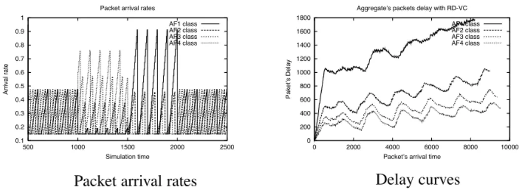
The graph on the left of figure 1 shows the arrival rates used for all classes. Every 500 time units3_{, the traffic}

characteristics change in order to have severe simulation conditions.

0.1 0.2 0.3 0.4 0.5 0.6 0.7 0.8 0.9 1 500 1000 1500 2000 2500 Arrival rate Simulation time Packet arrival rates

AF1 class AF2 class AF3 class AF4 class 0 200 400 600 800 1000 1200 1400 1600 1800 0 2000 4000 6000 8000 10000 Paket’s Delay

Packet’s arrival time Aggregate’s packets delay with RD-VC

AF1 class AF2 class AF3 class AF4 class

Packet arrival rates Delay curves

Figure 1: Per class delay curves for the RD-VC algorithm based on equation 13.

The right part of figure 1 shows the delays for each class for a stamp allocation based on equation 13. We note that the relative delays are assured and that delay curves are smooth4_{; which means that the delay variation, or}

jitter, is low for every class, while there are very important variations in the traffic loads in every class.

In the following section, we will show on other simulation results that the scheduler has an excellent behaviour, especially if we take into account that the stamps are fixed once and for all at packet arrival.

Moreover, this algorithme does not require one queue per class. When a single queue is used, it suffices to sort it by increasing stamp values, and to have two registers per class to store the size of the (logical) queue and the last stamp value assigned to a packet of this (logical) queue.

4 Simulations with fluid flows

The simulations in this section are carried out with fluid flows. The flows are termed as fluid because they have constant packet arrival rates i.e. the inter-packet time gap is uniform. Such flows are unrealistic for packet switched networks. The goal of these simulations is to investigate the performance of a delay-based scheduler under dif-ferent buffer loadings. In the next section 5, simulations will be performed using TCP flows yielding a realistic environment.

We simulate three schedulers: Ex-VC (section 2.2.1), WTP (section 2.1.3) and RD-VC (section 3). Our proposi-tion (RD-VC) is investigated for its performance under different loads and is compared with the existing Ex-VC

3_{A time unit represent the fixed-size packet transmission time.}

(11)

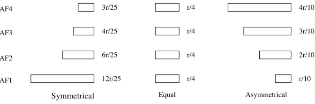
and WTP algorithms. We simulate four AF classes: AF1, AF2, AF3 and AF4. These classes have relative quality indices as: , , and . We define a warm-up period during which the rate of packet arrival is twice the packet service rate (i.e. the scheduler speed ). This makes the queue lengths grow. Once the warm-up period is over, the total rate of packet arrival becomes equal to the scheduler speed. Moreover, we define three scenarios of packets arrival: symmetrical, equal and asymmetrical (refer to figure 2).

In the symmetrical packets arrival scenario, the queues are loaded proportionally to their delay guarantees. That is to say that aggregate AF4 will receive packets at rate half of that at which aggregate AF2 would receive the packets. Recall that aggregate AF4 experiences half the delay of AF2.

In the equal packets arrival rate scenario, all aggregates receive packets at equal rates regardless of their quality indexes (i.e. delay guarantees).

The third scenario, asymmetrical packets arrival, tests an algorithm in tending-to-worst buffer loading con-figuration and algorithm self-regulates at a hard-going pace. Here, queues are loaded inversely proportional to their delay guarantees. In other words, the aggregate AF4 will receive packets at rate double of that at which aggregate AF2 would receive.

AF4 AF3 AF2 AF1 3r/25 4r/25 6r/25 12r/25 4r/10 3r/10 2r/10 r/10 r/4 r/4 r/4 r/4 Asymmetrical Equal Symmetrical

Figure 2: The rate of packet arrivals in three scenarios of buffer loadings

With three types of buffer loading during warm-up and post warm-up periods, we simulated nine scenarios for each of the three algorithms (Ex-VC, WTP, RD-VC). However, we present the simulation results only with equal packets arrival during the warm-up period. All results are shown on the same scale. The simulation parameters are: warm-up period is 500 packet slots, simulation time is 10000 packet slots, buffer over-loading factor during warm-up is 2 and service scheduler speed is 1 packet/time-slot.

4.1 Comparative study of delays per packet with three algorithms (Ex-VC, WTP, RD-VC)

An important common point to notice, in figure 3, is that all the three algorithms tend to respect the relative delay differentiation in all three post warm-up buffer loadings. Another common observation is that aggregates suffer, individually, more delays as the post warm-up loading changes from symmetrical to asymmetrical (horizontal move on each row of figure 3). However, the average delay per packet on the whole buffer is the same under all loads. The algorithms adapt themselves differently while reaching a stability. Though WTP takes shorter, it has certain implementation limitations, refer to section 2.3 for details. Moreover, it has some difficulties to respect

(12)

the delay differentiation during the warm-up period. This specificity will be detailed later in the WTP algorithm results analysis. 0 200 400 600 800 1000 1200 1400 0 1000 2000 3000 4000 5000 6000 7000 8000 9000 10000 Packet’s delay

Packet’s arrival time Delay Curves AF1 class AF2 class AF3 class AF4 class 0 200 400 600 800 1000 1200 1400 0 1000 2000 3000 4000 5000 6000 7000 8000 9000 10000 Packet’s delay

Packet’s arrival time Delay Curves

AF1 class

AF2 class AF3 class AF4 class

Warm-up: equal load, Post warm-up: symmetric load Warm-up: equal load, Post warm-up: equal load Warm-up: equal load, Post warm-up: asymmetric load a) Extended VC algorithm (EX-VC)

0 200 400 600 800 1000 1200 1400 0 1000 2000 3000 4000 5000 6000 7000 8000 9000 10000 Packet’s delay

AF1 class

Warm-up: equal load, Post warm-up: symmetric load Warm-up: equal load, Post warm-up: equal load Warm-up: equal load, Post warm-up: asymmetric load b) Waiting Time Priority algorithm (WTP)

0 200 400 600 800 1000 1200 1400 0 1000 2000 3000 4000 5000 6000 7000 8000 9000 10000 Packet’s delay

AF1 class

Warm-up: equal load, Post warm-up: symmetric load Warm-up: equal load, Post warm-up: equal load Warm-up: equal load, Post warm-up: asymmetric load c) Relative Delay VC algorithm (RD-VC)

Figure 3: Simulation results for delay per packet with the three algorithms

The Ex-VC algorithm: With equal rates of packet arrivals during the warm-up time, queues do not grow in

required relative sizes and the algorithm self-regulates significantly and takes a longer time to reach stabili-sation. We observe that Ex-VC is a little bit poor in performance as it takes more time to reach the stability and is more fluctuating [12]. This lack of performance is mainly due to the fact that the Ex-VC algorithm controls the delay per packet for an aggregate by adapting its service rate. This self-regulation is based on queue size of the aggregate rather than directly on delay. Moreover, packets are stamped at their arrivals. The state of the system at this time is not exactly the same as at the departure time of the packet.

However the algorithm is very simple because it does not need a separate queue per class but only one global queue. Only simple register are needed to memorize some values such as class queue size and class index.

(13)

The simplicity of the scheduler is considerable in the case of high speed networks with high speed routing systems.

The WTP algorithm: We see directly that this approach has the best performance among three algorithms.

Recall that mq-WTP is more complex and has limited implementation scope. It reaches rapidly to the sta-bility in all three post warm-up buffer loadings. The contributing factors are: 1) it controls the aggregate’s packet delays by considering the actual delays the packets are suffering, and 2) the packet stamp values are updated as they stay longer in the buffer to reflect the actual system state.

On the other hand, this approach does not respect the delay differentiation during the warm-up period. This phenomenon is observed on figure 3b, during the first 500 time periods of the simulation (the warm-up period). Typically, during high loads of the system, the WTP scheduler has to support too many classes requiring the best qualities, leaving of classes requiring lesser quality. Moreover, this approach suffers of two more disadvantages. The first one is the complexity. Indeed, the WTP algorithm needs a physical queue per traffic classes. The second one is the high processing cost, because each packet is treated twice: first the packet is stamped by the scheduler at its arrival, and second, when it arrives at the head of the queue, it is treated again to assign its priority.

The RD-VC algorithm: Our new approach is distinguished by its simplicity and its good performance.

Indeed, contrary to WTP, during the warm-up period, the relative delay differentiation is perfectly respected in relation with quality indices. When the period changes from the warm-up to post warm-up and after a short adaptation time, the algorithm becomes stable and provides again the required delay differentiation. It is not surprising that the transient phase is longer than with the WTP approach. RD-VC, like Ex-VC, stamps packets at their arrival depending on the current state of the system. Once packets are ready to be served, the state of the system has changed, and, contrary to the WTP algorithm, packet stamps are not recomputed. It is important to notice that, despite the non recalculation of the packet stamp and the strong input load variation, the RD-VC approach gives very good results.

4.1.1 Concluding remarks

The WTP scheduler seems to be the best among the three propositions (except under high load) but is restricted to switches with separate queues per aggregate architectures. On the other hand, the proposed RD-VC scheduler does not have this limitation and still has a performance which stays very close to WTP and is much better than the Ex-VC scheduler. Though Ex-VC does not seem to perform equally well, it has an advantage over WTP and RD-VC. If self-regulation is disabled, the Ex-VC scheduler would then perform the bandwidth based service differentiation among aggregates. Thus Ex-VC can easily be made to work in two modes of service differentiation which is not the case with WTP and RD-VC. Finally, selecting a scheduler among these three entirely depends upon the available switch architectures and service modes.

(14)

5 Simulations with TCP flows

In the last section, we showed, by using fluid flows, that all three schedulers (Ex-VC, WTP and RD-VC) maintain the service differentiation among aggregates at all loads. We now proceed further in our studies by using realistic flows and use the STCP [13] simulator, which has a very accurate model of TCP. We implement an AF-like PHB which comprises a packet accept/discard algorithm and a packet scheduler.

5.1 Implementing Relative Quantification Services in DiffServ

A relative quantification service [7] quantifies the forwarding assurance of an aggregate with respect to the service given to other aggregates. For example, an aggregate A gets times the service given to the aggregate B. We define an AF-like PHB to provide this service in a simulated DiffServ domain. This PHB constitutes a packet accept/discard algorithm and a packet scheduling algorithm. In the sequel, we show results with RED as packet discard algorithm and Ex-VC, WTP and RD-VC as schedulers.

5.2 Simulating parameters of STCP

The simulations were performed with the STCP simulator [13]. The TCP workstations are connected to IP routers which are then interconnected by an ATM backbone. The TCP sources transmit short files of 200Kbytes without inter file delay. The slow time-out is 200ms (the maximum delay between two consecutive delayed ACKs) whereas fast time-out is 50ms (instead of traditionally used 500ms timer). The Maximum Segment Size (MSS) is 1460 bytes and maximum window size is 64Kbytes. The Selective ACKnowledgement (SACK) option is enabled. The simulation duration is fixed to 102 seconds. We use RED as packet accept/discard with min th=1000, max th=7000

(cells), and .

Among eight simulated configurations of four scenarios, we present here only one scenario configuration described in the following section.

(15)

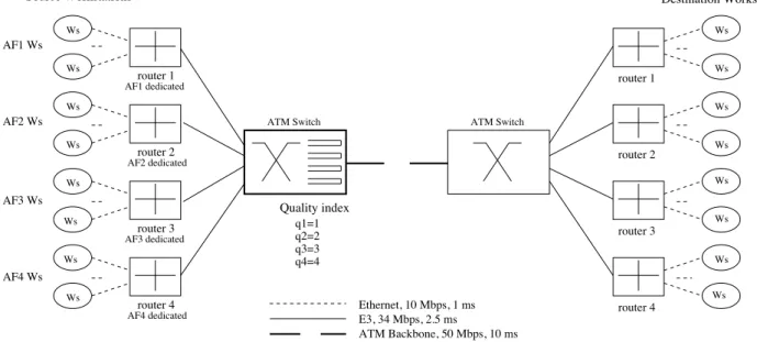
5.2.1 Basic simulation scenario AF1 Ws Ethernet, 10 Mbps, 1 ms E3, 34 Mbps, 2.5 ms ATM Backbone, 50 Mbps, 10 ms AF3 Ws AF4 Ws router 1 router 2 router 3 router 4 Quality index q1=1 q2=2 q3=3 q4=4 Ws Ws Ws Ws Ws Ws Ws Ws Ws Ws Ws Ws Ws Ws Ws Ws router 1 router 2 router 3 router 4

Source Workstations _{Destination Workstations}

AF1 dedicated

AF2 dedicated

AF3 dedicated

AF4 dedicated

AF2 Ws ATM Switch ATM Switch

Figure 4: The basic simulation scenario.

In this scenario, as shown in figure 4, 200 pairs of TCP sources are interconnected via four routers and two ATM switches forming the backbone. Each of the four routers is dedicated to a certain AF class as shown. The backbone is at 50Mbps and has a transmission delay of 10ms. The ATM switch performs service differentiation among aggregates in accordance with their respective quality indices. We perform three types of loadings per aggregate:

Symmetrical loading: The aggregates are loaded proportionally to their (relative) delay guarantees. That

is to say that aggregate AF4 will receive packets, on the average, at rate half of that at which aggregate AF2 would receive the packets. Recall that aggregate AF4 experiences half the delay of AF2. The symmetric loading is simulated by having 80 workstations (1 TCP flow per workstation) for AF1 (i.e. attached to router 1), 60 for AF2, 40 for AF3 and 20 for AF4.

Equal loading: All aggregates are loaded with equal rates regardless of their quality indexes. Here, the

basic scenario contains 50 workstations for each AF class.

Asymmetrical loading: Aggregates are loaded inversely proportionally to their delay guarantees. In other

words, the aggregate AF4 will receive packets, on the average, at rate double of that at which aggregate AF2 would receive. The class AF1 is fed with 20 TCP flows, AF2 with 40, AF3 with 60 and AF4 with 80 flows. The purpose of having three different buffer loadings in basic scenario is to verify the following two points: 1. The service differentiation among the aggregates is respected at all loads.

2. The packet loss ratio (PLR) is the same for all the aggregates as RED is implemented at head queue, not on individual queues.

(16)

We use three schedulers (Ex-VC, WTP and RD-VC) alternatively and present the results in three different tables.

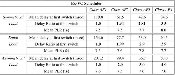
Table 1: Results table for basic scenario: Ex-VC Scheduler.

Ex-VC Scheduler

Class AF1 Class AF2 Class AF3 Class AF4

Symmetrical Mean delay at first switch (msec) 119.8 61.5 42.6 34.6

Load Delay Ratio at first switch 1.0 1.94 2.81 3.5

Mean PLR (%) 7.5 7.5 7.7 8.0

Equal Mean delay at first switch (msec) 154.6 77.7 53.0 40.5

Mean PLR (%) 7.5 7.6 7.8 7.7

Asymmetrical Mean delay at first switch (msec) 201.2 99.4 66.7 50.0

Mean PLR (%) 7.6 7.5 7.6 7.6

Table 2: Results table for basic scenario: WTP Scheduler.

WTP Scheduler

Mean PLR (%) 7.9 7.5 7.3 7.3

Mean PLR (%) 8.0 7.8 7.5 7.3

(17)

Table 3: Results table for basic scenario: RD-VC Scheduler.

RD-VC Scheduler

Load Delay Ratio at first switch 1.0 2.1 3 3.9

Mean PLR (%) 7.4 7.5 7.8 7.9

Mean PLR (%) 7.4 7.5 7.5 7.4

Mean PLR (%) 7.6 7.5 7.8 7.8

The tables 1, 2 and 3 show the mean local delays at the left backbone switch and the ratio between these delays for each scheduler. With the ratio information, we can conclude that the delay differentiation follows closely the aggregate’s quality indices under all loading configurations for all three schedulers. However, Ex-VC does not seem to perform very well under symmetrical loading, see table 1. The aggregate AF4 is lightly loaded and its queue length does not grow significantly. Since Ex-VC works on queue length (self-regulation), the aggregate AF4 (and AF3 also to some extent) does not fully attain their deserved service.

In case of a scheduler, say the Ex-VC algorithm, the values of mean global buffer (sum of four AF aggregates) occupancy, at switch, in symmetrical, equal and asymmetrical loading configurations are (in cells): 9.06K, 9.08K and 9.05K respectively. Since the mean buffer occupancy at switch is the same for all the configurations and the server is work conserving, the average delay per packet per global buffer is the same for all the configurations. However, we notice in table 1, that aggregates suffer, on the average, individually more delays as we move from symmetrical to asymmetrical buffer loading. The same is observed for the other two schedulers too.

The same tables 1, 2 and 3 present also the mean Packet Loss Ratio (PLR) per aggregate.

These PLR values are approximately the same for all the aggregates under a given loading configuration. For example under equal load and for the EX-VC scheduler (table 1), the PLRs are 7.5, 7.6, 7.8 and 7.7 for AF1, AF2, AF3 and AF4 respectively. This is due to having a packet accept/discard algorithm (RED) on the head queue.

In conclusion, we can see that the expected discrimination over delays is obtained, while maintaining the same loss rates. Therefore, TCP flows in classes with lower delays will get more throughput, independently from the load in their class, since the TCP throughput is inversely proportional to the RTT and to the square root of the packet loss rate.

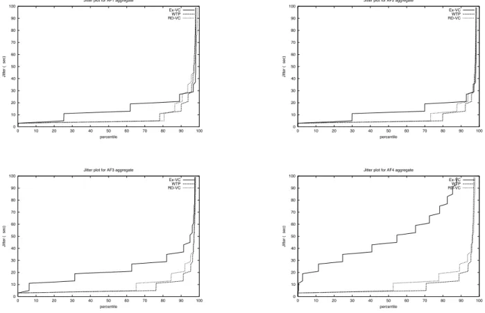
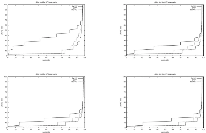
5.2.1.1 Jitter evaluation: It seems from the tables 1, 2 and 3 that all three schedulers have comparable

per-formance. It should be noted that tables present an average performance based on a long-term observation. Let us look at the jitter performance of three schedulers in the basic simulation scenario of figure 4. The jitter reflects the

(18)

instantaneous packet delay variation and helps compare the short-term performance of schedulers. Note that all three schedulers provide the required service differentiation among aggregates, though they yield different jitters. It means that average values of delay per packet for each aggregate are very close in all three schedulers but the variation from these average values per aggregate will differ from one scheduler to other. Jitter is measured as:

(18) We plot jitter as percentile for each AF aggregate with three schedulers. The plots show that WTP and RD-VC have comparable jitter performance whereas Ex-VC does not perform well in some cases, for example look at figure 5 for AF4 aggregate and at figure 7 for AF1 aggregate. This jitter-focused study proves that the WTP and RD-VC schedulers take an edge over Ex-VC especially for applications where performance at short scale is also important in addition to that at larger scale (the average service differentiation).

0 10 20 30 40 50 60 70 80 90 100 0 10 20 30 40 50 60 70 80 90 100 Jitter ( sec) percentile Jitter plot for AF1 aggregate

Ex-VC WTP RD-VC 0 10 20 30 40 50 60 70 80 90 100 0 10 20 30 40 50 60 70 80 90 100 Jitter ( sec) percentile Jitter plot for AF2 aggregate

Ex-VC WTP RD-VC

(19)

Ex-VC WTP RD-VC

Figure 6: Jitter evaluation for the basic scenario: equal load

Ex-VC WTP RD-VC

(20)

6 Conclusion

The role of a packet scheduler becomes more important when the service differentiation is performed at aggregate level. The service differentiation needs to be done in a way that the same quality is delivered at microflow level as that at aggregate level. Among the three possible quality metrics for service differentiation namely bandwidth, loss and delay; bandwidth requires microflow aware management, loss-based differentiation is too tedious to manage and delay appears as a good candidate. A better delay at aggregate level means better delay for all its microflows. Three existing approaches (BPR, Ex-VC and WTP) were presented and compared. Afterwards, we proposed our new approach named RD-VC and it was compared to all other algorithms graphically and numerically.

It arises that WTP approach adapts itself more rapidly than BPR, EX-VC or RD-VC. However, WTP has some difficulties to respect relative delay differentiation during high load and is more complex to implement in high speed devices. RD-VC seems to be the best compromise between performance and simplicity. It has two important characteristic: 1) it does not require to maintain separate queues per class and can be implemented with a single queue buffer accommodating all classes, 2) packet are stamped once at their arrival and their stamp values are not changed or updated, hence its operational cost per packet is constant. This second characteristic is the most important to us.

We implement these three schedulers (RD-VC, WTP and Ex-VC) as a part of an AF PHB in a Differentiated Services network. We perform a comparative study and find that the three schedulers maintain the required service differentiation among Aggregates. However, WTP and RD-VC take an edge over Ex-VC at short-term perfor-mance like jitter. Both WTP and RD-VC have good long term and short-term perforperfor-mance.

7 Acknowledgements

We would like to thank Olivier Bonaventure for interesting comments on an earlier version of this paper. This work has been carried out within the IST ATRIUM project partially funded by the European Commission.

(21)

References

[1] R. Guerin and V. Peris, “Quality of Service in Packet Networks - Basic Mechanims and Directions,” Computer Networks and ISDN Systems, special issue on multimedia communications over packet based networks , 1998.

[2] L. Kleinrock, “A Delay Dependent Queue Discipline,” Nav. Res. Log. Quart. 9, pp. 31–36, 1962.

[3] C. Dovrolis and D. Stiliadis, “Proportional Differentiated Services: Delay Differentiation and Packet Scheduling,” Proceedings of ACM SIGCOMM-99, (http://www.cae.wisc.edu/ dovrolis/) , 1999.

[4] M. Tufail, G. Jennes, and G. Leduc, “A scheduler for delay-based service differentiation among AF classes,” Proc. of IFIP Fifth International Conference on Broadband Communications’99, Boston, Kluwer Academic Press , pp. 93–102, Nov. 1999.

[5] S. Blake, D. Black, M. Carlson, E. Davis, Z. Wang, and W. Weiss, “An Architecture for Differentiated Services,” Internet RFC 2475 .

[6] J. Heinanen, T. Finland, F. Baker, W. Weiss, and J. Wroclawski, “Assured Forwarding PHB Group,” Internet RFC 2597 , 1999.

[7] Y. Boram, J. Binder, S. Blake, M. Carlson, B. E. Carpenter, S. Keshave, E. Davies, B. Ohlman, D. Verma, Z. Wang, and W. Weiss, “A Framework for Differentiated Services,” Internet draft: draft-ietf-diffserv-framework-02.txt , Feb. 1999. [8] P. Hurley and J. Y. L. Boudec, “A proposal for an Asymmetric Best-Effort Service,” Proceedings of 1999 Seventh

International Workshop on Quality of Service (IWQoS’99), also available as SSC technical report SSC/1999/003 at http://icawww.epfl.ch , pp. 132–134, London, England, May 1999.

[9] Y. Moret and S. Fdida, “A proportional Queue Control Mechanism to Provide Differentiated Services,” International Symposium on Computer System, Belek, Turkey , Oct. 1998.

[10] A. K. Parekh and R. G. Gallager, “A Generalized Processor Sharing Approach to Flow Control in Integrated Services Networks: The Single-Node Case,” IEEE/ACM Transactions on Networking, Vol. 1 , pp. 344–357, June 1993.

[11] S. D. Cnodder and K. Pauwels, “Relative delay priorities in a differentiated services network architecture,” Alcatel Alsthom CRC (Antwerp, Belgium) deliverable , 1999.

[12] M. Tufail, G. Jennes, and G. Leduc, “Providing a DiffServ like service in ATM networks,” Alcatel Alsthom CRC (Antwerp, Belgium) IWT Deliverable , Oct. 1999.