Reconfiguration in Stochastic Petri Nets

Ministère de l’Enseignement Supérieur et de la Recherche Scientifique Université Mohamed Khider – BISKRA

N° d’ordre :... Série :...

Faculté des Sciences Exactes et des Sciences de la Nature et de la Vie Département d’Informatique

THÈSE

Présentée pour obtenir le diplôme de

DOCTORAT EN SCIENCES EN INFORMATIQUE

Par

Samir TIGANE

THÈME

Reconfiguration in Stochastic Petri Nets

Devant le jury composé de :

Pr. Kazar Okba Président Professeur à l’Université de Biskra. Pr. Kahloul Laïd Rapporteur Professeur à l’Université de Biskra. Dr. Baarir Souheib Co-Rapporteur Maitre de Conférences Habilité à

l’Université Paris Ouest Nanterre. Pr. Bennoui Hamadi Examinateur Professeur à l’Université de Biskra.

Pr. Chaoui Allaoua Examinateur Professeur à l’Université de Constantine 2. Pr. Saidouni Djemal Eddine Examinateur Professeur à l’Université de Constantine 2.

ﻞ ﺸ ﺔﻄﺑا ﻣو ﺔﻴﻜﻴﻣﺎﻨﻳد ﺔﻴ ﺑ تاذ و ﺪﻳا ﻣ ﻞ ﺸ ةﺪﻘﻌﻣ ﺔﻠﺼﻔﻨﳌا ثاﺪﺣ ﺔﻤﻈﻧأ ﻦﻣ ﺪﻳﺪﻌﻟا ﺖﺤﺒﺻأ ،ةﺮﺻﺎﻌﳌا ﺎﻨﻣﺎﻳأ

ﺮﻳﺎﻐﺘﻣ

.

ﺎ ﻴ ﺑ ﻴﻐ ﻦﻣ ﻦﻜﻤﺘﺘﻟ ﺔﻤﻈﻧ ﻩﺬ ﻢﻴﻤﺼﺗ ﻢﺗ ﺪﻘﻠﻓ

ﻞﻴﻐﺸ ﻟا ﺖﻗو ،

ءاﺰﺟ ﺾﻌ ﺔﻟازإ وأ ﺔﻓﺎﺿإ ﻖ ﺮﻃ ﻦﻋ ،

،

او فوﺮﻈﻟا ﻊﻣ ﻒﻴﻜﺘﻟا ﻦﻣ ﺎ ﻴﻜﻤﺘﻟ

ةﺪﻳﺪ ا تﺎﺒﻠﻄﺘﳌ

.

ﺔﻴﻤﺳر ةادﺄ

ﺔﻤﻈﻧ ﻩﺬ ﻞﺜﻣ ﺔﺳارد ي ﺑ تﺎ ﺒﺷ ماﺪﺨﺘﺳا ،

ن ﺜﺣﺎﺒﻟا ﻦﻣ ﺪﻳﺪﻌﻟا بﺬﺠﻳ

.

ﺔ ﻮﻗ ةادأ ﻞﺜﻤﺗ ي ﺑ تﺎ ﺒﺷ نأ ﻦﻣ ﻢﻏﺮﻟا ﻋ

ﺔﻣﺪﻘﺘﳌا ﺔﻤﻈﻧ ﻦﻣ ﺔﺴﻠﺳ ﺔﻘ ﺮﻄﺑ ﻖﻘﺤﺘﻟا و ﺪﻳﺪﺤﺘﻟا ﻋ ةردﺎﻗ ﻏ ﺎ أ ﻻإ ،

ﺔﻴﻜﻴﻣﺎﻨﻳﺪﻟا ﺔﻴ ﺒﻟا تاذ

.

ﻊﻗاﻮﻟا

،

ﺔﺒﻠﻘﺘﳌا تﺎﺌ ﺒﻟا ﻢﻋﺪﺗ ﻟا ﺔﻤﻈﻧ

ةﺮﻤﺘﺴﳌا تا ﻐﺘﻟاو ،

ﻞﻴﻜﺸ ﻟا ةدﺎﻋﻹ ﺔﻠﺑﺎﻘﻟا ﻞ ﺎﻴ ﻟاو ،

ﺔﻳﺎﻐﻠﻟ ةﺪﻘﻌﻣ

.

ﺔﻠ ﺸﳌا ﻩﺬ ﻋ ﺐﻠﻐﺘﻠﻟ

ﻞﻴﻜﺸ ﻟا ةدﺎﻋإ ﺔﻴﺻﺎﺨﺑ ي ﺑ تﺎ ﺒﺷ ن ﺜﺣﺎﺒﻟا ﻦﻣ ﺪﻳﺪﻌﻟا ىﺮﺛأ ،

.

نﺈﻓ ،ﻚﻟذ ﻊﻣو

راﺮﻘﻟا ةﻮﻗ ﻦﻣ ﻞﻠﻘﻳ ﺔﺟﺬﻤﻨﻟا ةﻮﻗ ةدﺎز

.

ﻊﻗاﻮﻟا

ﻦﻣ ﺪﻳﺪﻌﻟا ،

ﻘﺘﻠﻟ ﺔﻠﺑﺎﻗ ﻏ ﺢﺒﺼﺗ ﺺﺋﺎﺼ ا

.

ﻚﻟﺬﻟ

ﺔﺟﺬﻤﻨﻟا تﺎ ﻮﺘﺴﻣ ن ﺑ ﻂﺳو ﻞﺣ دﺎﺠﻳإ ي ﺑ تﺎ ﺒﺷ إ ﻞﻴﻜﺸ ﻟا ةدﺎﻋإ ﻞﺧﺪﺗ ﻟا ﺔﺣ ﻘﳌا تﺎﻓﺎﺿ لوﺎﺤﺗ ،

ﻖﻘﺤﺘﻟاو

.

ﺔﺣوﺮﻃ ﻩﺬ

قﺮﻃ ﺔﺛﻼﺛ ﻢﻳﺪﻘﺘﺑ مﻮﻘﻨﺳ ،

-

ً

ﺎﻴﺠرﺪﺗ ﺎ ﺮ ﻮﻄﺗ ﻢﺗ

-

ﻴﺑ تﺎ ﺒﺷ ﻦ ﻮ ﺘﻟا ةدﺎﻋإ ﻦﻣ ﻖﻘﺤﺘﻟاو ﺔﺟﺬﻤﻨﻠﻟ

ي

ﺔﻤﻤﻌﳌا ﺔﻴﺋاﻮﺸﻌﻟا

(GSPNs)

ﮫ ﺎﺠﺗاو ﻩدوﺪﺣو ﻩﺎﻳاﺰﻣ ﮫﻟ ﺎ ﻣ ﻞ ،

ﻦﻣ ﺪﻳﺪﻌﻟا ﻦﻣ ﻖﻘﺤﺘﻟا ﺔﻴﻧﺎ ﻣإ ﻋ ظﺎﻔ ا ﻊﻣ ،

ﻞﻗأ ﺪﻴﻘﻌ ﻊﻣ ﺺﺋﺎﺼ ا

.

ً

ﻻوأ

ﺔﻴﻠ ﺷ ح ﻘﻧ ،

ﺴ ،

GSPNs

ﺔﺑﺎﺘﻜﻟا ةدﺎﻋﻹ ﺔﻠﺑﺎﻗ ﺎﻴﺟﻮﻟﻮﺒﻃ ﻊﻣ

(GSPNs-RT)

ﺎﻴﺟﻮﻟﻮ ﻮﻃ ﺔﺟﺬﻤﻨﺑ ﺢﻤﺴ ﻟاو ،

ﻞ ﻮﺤﺗو ﺔﻴﻜﻴﻣﺎﻨﻳد

GSPNs-RT

إ

GSPNs

ﺔﺌﻓﺎ ﻣ

ةﺰ ﺎ ا ﻖﻘﺤﺘﻟا تاودأ ﻦﻣ ﺔﻠﻣﺎ ﻟا ةدﺎﻔﺘﺳ ﻞﺟأ ﻦﻣ ،

.

ﻚﻟذ ﺪﻌ

ىﺮﺧأ ﺔﻴﻠ ﺷ ح ﻘﻧ ،

ﺴ ،

GSPNs

ﺔﻴﻜﻴﻣﺎﻨﻳﺪﻟا

(D-GSPNs)

ﻞ ﺎﻴ ﻟا ﻦﻣ ﻖﻘﺤﺘﻟاو ﺔﺟﺬﻤﻨﻟﺎﺑ ﺢﻤﺴ ﻟاو ،

ﺔﻴﻜﻴﻣﺎﻨﻳﺪﻟا

)

ﺔﻴﻜﻴﻣﺎﻨﻳد تﻻﺎﻘﺘﻧ و ﻦﻛﺎﻣ تﺎﻋﻮﻤﺠﻣ نأ ﺚﻴﺣ

(

ﻞ ﻮﺤﺘ و

D-GSPNs

إ

GSPNs

ﺔﺌﻓﺎ ﻣ

.

ﻩﺬ ﻟ ﻦﻜﻤﻳ

تﺎﻨ ﻮ ﺘﻟا ﻦﻣ ادﺪﺤﻣ ادﺪﻋ ﺔﻴﻠﺻ جذﺎﻤﻨﻟا ﻚﻠﺘﻤﺗ ﺎﻣﺪﻨﻋ ثﺪﺤﺗ نأ تﻼ ﻮﺤﺘﻟا

.

اً ﺧأ

رﻮﻄﺗ ،

GSPNs

ﻞﻴﻜﺸ ﻟا ةدﺎﻋﻹ ﺔﻠﺑﺎﻗ ﺔﻴﻠ ﺷ إ

ﺴ ،

GSPNs

ﻦ ﻮ ﺘﻟا ةدﺎﻋﻹ ﺔﻠﺑﺎﻘﻟا

(RecGSPNs)

ﻢﻋﺪﺗ ﻟاو ،

حﻮﻤﺴﻣ ﻮ ﺎﻤﺑ ﺔﻴﻠ ﻴ ﻟا تا ﻴﻐﺘﻟا ﻦﻣ ﻛأ ﺔﻋﻮﻤﺠﻣ

ﺔﻴﻟﺎ ا ﺐﻴﻟﺎﺳ ﮫﺑ

ﻚﻟﺬﻛو ،

يﻷ ﺢﻤﺴ ،

GSPN

ﻦ ﻮ ﺘﻠﻟ ﺔﻠﺑﺎﻗ

ﺔﻣﺎ ﻟا ﺺﺋﺎﺼ ا ﻦﻣ ﺪﻳﺪﻌﻟا ﻦﻣ ﻖﻘﺤﺘﻟا ﺔﻴﻠﺑﺎﻗ ﻋ ظﺎﻔ ا ﻊﻣ تﺎﻨ ﻮ ﺘﻟا ﻦﻣ ﮫﻟ ﺮﺼﺣ ﻻ دﺪﻋ ﻋ لﻮﺼ ﺎﺑ

.

ﺔﻴﺣﺎﺘﻔﳌا تﺎﻤﻠ ﻟا

:

ﺔﻤﻤﻌﳌا ﺔﻴﺋاﻮﺸﻌﻟا ي ﺑ تﺎ ﺒﺷ

ﺔﻴﻜﻴﻣﺎﻨﻳﺪﻟا ﻞ ﺎﻴ ﻟا و جذﺎﻤﻨﻟا

-

ﻟا ﻞ ﻮﺤﺗ ﺔﻤﻈﻧأ

جذﺎﻤﻨ

-

ي ﺑ تﺎ ﺒﺷ

ﺔﻜﻠﻴ ﻟا ةدﺎﻋﻹ ﺔﺒﻟﺎﻘﻟا

ﻜﺸﻟا ﻖﻘﺤﺘﻟا و ﺔﺟﺬﻤﻨﻟا

ءاد ﻢﻴﻴﻘﺗ

.

Nowadays, many discrete event systems (DESs) are becoming increasingly complex, struc-turally dynamic and variably interconnected. These systems are designed to be able to change their structure and/or topology, at run-time, to accommodate new circumstances/require-ments. As a formal tool, the use of Petri nets (PNs) in the study of such systems attracts many researchers.

Although PNs (low or high) are a powerful and expressive tool, they are unable to spec-ify/verify, in a natural way, advanced systems having dynamic structures. Indeed, systems supporting volatile environments, continuous variations, and reconfigurable structures are expected to be extremely complex. To overcome this issue, researchers enrich PNs with reconfigurability. Nevertheless, increasing the modeling power of a formalism decreases its decision power. In fact, several properties become undecidable. Therefore, extensions pro-posed in the literature introducing reconfigurability to PNs try to find a compromise between the modeling and the verification levels.

In this thesis, we describe three approaches – incrementally developed – for the model-ing and verification of reconfiguration in generalized stochastic Petri nets (GSPNs), while maintaining verifiability of several properties with reduced complexity.

First, we propose a formalism, called GSPNs with rewritable topology (GSPNs-RT), that extends GSPNs by allowing modeling dynamic topologies and transforming GSPNs-RT to equivalent GSPNs, to take full advantages of off-the-shelf tools proposed for GSPNs verification.

Then, we propose another formalism, called dynamic GSPNs (D-GSPNs), that allows modeling and verifying dynamic structures (sets of places and transitions are dynamic) and transforms D-GSPNs to equivalent GSPNs. This transformation can take place when the original model disposes of a finite number of configurations.

Finally, GSPNs are extended to a reconfigurable formalism, called reconfigurable GSPNs (RecGSPNs), that supports a wider range of possible structural changes than allowed in existing approaches, as well as, allows to any RecGSPN to have an infinite number of con-figurations while preserving the decidability of several important properties.

Keywords: Generalized stochastic Petri nets; Dynamic model and structure; Graph transformation systems; Formal modeling and verification; Performance evaluation.

De nos jours, de nombreux systèmes à événements discrets deviennent de plus en plus com-plexes, structurellement dynamiques et interconnectés de manière variable. Ces systèmes sont conçus pour pouvoir modifier leur structure et/ou leur topologie, au moment de l’exé-cution, afin de s’adapter à des nouvelles circonstances/exigences. En tant qu’outil formel, l’utilisation de réseaux de Petri dans l’étude de tels systèmes attire de nombreux chercheurs. Bien que les réseaux de Petri (bas ou haut niveau) constituent un outil puissant et ex-pressif, ils ne sont pas en mesure de spécifier/vérifier, de manière naturelle, des systèmes avancés dotés de structures dynamiques. En effet, les systèmes prenant en charge des en-vironnements volatils, des variations continues et des structures reconfigurables devraient être extrêmement complexes. Pour surmonter ce problème, les chercheurs enrichissent les réseaux de Petri avec la reconfigurabilité. Néanmoins, augmenter le pouvoir de modélisation d’un formalisme diminue son pouvoir de décision. En fait, plusieurs propriétés deviennent indécidables. Par conséquent, les extensions proposées dans la littérature introduisant la reconfigurabilité dans les réseaux de Petri tentent de trouver un compromis entre les niveaux de modélisation et de vérification.

Dans cette thèse, on définit trois approches – développées incrémentalement – pour la modélisation et la vérification des réseaux de Petri stochastiques généralisés (GSPNs) re-configurables, tout en maintenant la vérifiabilité de plusieurs propriétés avec une complexité réduite.

En premier lieu, on propose un formalisme, appelé GSPNs avec topologie modifiable (GSPNs-RT), qui étend les GSPNs en permettant la modélisation de topologies dynamiques et la transformation de GSPNs-RT en GSPNs équivalents, afin de tirer pleinement d’avan-tages des outils standard proposés pour la vérification des GSPNs.

Ensuite, on propose un autre formalisme, appelé GSPNs dynamiques (D-GSPNs), qui permet de modéliser des structures dynamiques (les ensembles de places et de transitions sont dynamiques) et transforme les D-GSPNs en GSPNs équivalents. Cette transformation peut avoir lieu lorsque le modèle original disposent d’un nombre fini de configurations.

Enfin, on étend les GSPNs à un formalisme reconfigurable, appelé GSPNs reconfigurable (RecGSPNs), qui prend en charge une plus large gamme de changements structurels possi-bles que ce qui est autorisé dans les approches existantes, ainsi que, permet à tout GSPN reconfigurable d’avoir un nombre infini de configurations tout en préservant la décidabilité de plusieurs propriétés importantes.

Mot-clés : Réseaux de Petri stochastiques généralisés ; Modèle et structure dynamiques; Système de transformation de graphes ; Modélisation et vérification formelles ; Évaluation de performance.

Dedication

This thesis is dedicated to.... My beloved mother for her great support, love, pray, and care. My valuable treasures in my life: family and friends.

Acknowledgment

I would like to express my sincere gratitude to my supervisors Laid Kahloul and Souheib Baarir for their constant guidance, support, and encouragement.

I have to thank also all the team in LIP6 (Paris 6) in which I had the chance to pass one year during the finalization of this thesis.

Special thanks to Prof. Kazar Okba who always offers his unlimited support to the members of LINFI laboratory.

Finally, I would like also to present my thanks to the members of the jury who give me the honor by accepting to evaluate and review this work.

Contents

1 Introduction 1

Background . . . 1

Motivation and Objectives . . . 4

Contributions . . . 5

Thesis Organization . . . 7

I State-of-the-Art

9

2.2 Modeling with Petri nets . . . 12

2.3 Petri Net Structure . . . 13

2.4 Dynamic Behavior of Petri Nets . . . 14

2.5 Petri Net Analysis . . . 17

2.5.1 Petri Net Properties . . . 17

2.5.2 Temporal Logic . . . 21

2.5.3 Analysis Methods . . . 23

2.6 Stochastic Petri Nets . . . 24

2.6.1 Stochastic Process . . . 26

2.6.2 Markov Process . . . 26

2.6.3 Stochastic Petri Nets having Exponential Law . . . 27

2.6.4 Quantitative Properties . . . 30

2.7 Generalized Stochastic Petri Nets . . . 31

2.7.1 Embedded Markov Chain . . . 33

2.8 Conclusion . . . 36

3 Reconfiguration in Petri Nets 37 3.1 Introduction . . . 38

3.4 Net Rewriting Systems . . . 42

3.5 Self-Modifying Nets . . . 45

3.6 Reconfigurable Petri Nets . . . 46

3.7 Improved Net Rewriting Systems . . . 49

3.8 Other Extensions . . . 51

3.9 Trade-off between Expressiveness and Calculability . . . 52

3.10 Conclusion . . . 53

II Contributions

55

4.2 GSPNs with rewritable topology . . . 57

4.2.1 Formal definition . . . 58

4.3 Proofs . . . 61

4.4 Illustrative Example . . . 62

4.5 Conclusion . . . 67

5 Dynamic Generalized Stochastic Petri Nets 68 5.1 Introduction . . . 69 5.2 Dynamic GSPNs . . . 70 5.2.1 Formal definition . . . 70 5.3 D-GSPNs transformation towards GSPNs . . . 71 5.4 Qualitative/Quantitative Analysis of D-GSPNs . . . 75 5.5 Proofs . . . 76 5.6 Illustrative example . . . 79 5.7 Conclusion . . . 84

6 Reconfigurable Generalized Stochastic Petri Nets 85 6.1 Introduction . . . 86

6.2 Reconfigurable Generalized Stochastic Petri Nets . . . 87

6.2.1 Definition of RecGSPNs . . . 87

6.2.2 Properties Preserving Nets . . . 92

6.3 Preservation of properties in RecGSPNs . . . 93

6.3.1 Preservation of LBR, home state, and deadlock-free . . . 93

6.3.2 Preservation of linear temporal properties . . . 98

6.6 Conclusion . . . 109

7 Discussion 110 7.1 Introduction . . . 111

7.2 Qualitative Aspects . . . 111

7.3 Quantitative Aspects . . . 114

7.3.1 Factor 1: Model size . . . 115

7.3.2 Factor 2: Markov chain spatial complexity . . . 118

7.3.3 Factor 3: Markov chain time complexity . . . 119

7.4 Conclusion . . . 120

8 Conclusion 122 Appendices 126 A A Prototype for RecGSPNs 126 A.1 Introduction . . . 127 A.2 Description . . . 127 A.2.1 Place . . . 127 A.2.2 Transition . . . 127 A.2.3 Rule . . . 128 A.2.4 GSPN . . . 129 A.2.5 RecGSPN . . . 131 A.3 Demonstration . . . 132 A.4 Conclusion . . . 136 List of Publications 137 Bibliography 138

List of Figures

2.1 A PN models mutual exclusion. . . 13

2.2 Firing transitions in PN H at M0. . . 16

2.3 Reachability graph of H. . . 17

2.4 Different levels of liveness. . . 18

2.5 Conservation, persistence and fairness. . . 20

2.6 Transition system of H. . . 22

2.7 SPN N models mutual exclusion. . . 28

2.8 Corresponding CTMC of SPN N . . . 29

2.9 GSPN G models mutual exclusion. . . 32

2.10 Corresponding stochastic process of GSPN G. . . 33

3.1 PN morphisms. . . 40

3.2 DPO diagram. . . 41

3.3 NRS rule r0. . . 43

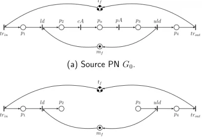
3.4 An application of NRS rule r0 to G0. . . 44

3.5 Self-modifying nets. . . 45

3.6 Reconfiguration after applying r. . . 47

3.7 Equivalent PN to RPN N. . . 49

3.8 Net block library. . . 50

3.9 Compromise between modeling and decidability. . . 53

4.1 Reconfiguration of RPN N. . . 58

4.2 Counterexample 1. . . 58

4.3 Counterexample 2. . . 58

4.4 First configuration. . . 62

4.5 GSPN model for configuration C1. . . 64

4.6 Equivalent GSPN Ge. . . 66

4.7 Probability that the current configuration is C0 or C1. . . 66

4.8 Probability that VM1/VM2 is working. . . 67

5.3 Equivalent GSPN H0 to D-GSPN D0. . . 72

5.4 Reachability graph of equivalent GSPN H0. . . 77

5.5 Reachability graph of D-GSPN D0. . . 78 5.6 Initial configuration C0. . . 79 5.7 Rule r1. . . 80 5.8 Configuration C1 (Alternative 1). . . 81 5.9 Rule r2. . . 81 5.10 Rule r3. . . 81 5.11 Rule r4. . . 81 5.12 Configuration C2. . . 82 5.13 The transformation of D1. . . 82 5.14 The transformation of D2. . . 83

5.15 Throughput of A and B productions. . . 83

6.1 Morphism. . . 88

6.2 Steps of applying a rewriting rule. . . 89

6.3 Reconfiguration in RecGSPNs. . . 91

6.4 Properties preserving nets examples. . . 92

6.5 Reachability graphs of both configurations C0 and C1. . . 95

6.6 Mutual exclusion. . . 99

6.7 Transition systems of GSPNs H and H0. . . 99

6.8 semi-Markov chain of Ψ0. . . 103

6.9 GSPN model of LM. . . 106

6.10 Left and right-hand sides of r1. . . 107

6.11 Left and right-hand sides of r3. . . 108

6.12 Performance evaluation of the RMS. . . 109

7.1 Modeling versus Decidability . . . 114

7.2 GSPN models of initial and second configurations. . . 115

7.3 Model of reconfigurable system based on classical approaches. . . 116

7.4 Model of reconfigurable system based on D-GSPNs. . . 117

7.5 Model size. . . 118

7.6 Time to compute Markov chain. . . 119

A.1 Initial configuration. . . 133

A.2 Left-hand side of rule r1 and right-hand side of rule r2. . . 133

List of Tables

2.1 Reachable markings of H. . . 17

2.2 Reachable markings of G. . . 33

4.1 Entry of the different evaluations. . . 65

5.1 Reachability set of H0. . . 78

5.2 Reachability set of D0. . . 78

5.3 Meaning of places and transitions in configuration C0. . . 80

5.4 Transition rates in both alternatives. . . 83

6.1 State space of semi-Markov chain depicted in Fig. 6.8. . . 104

7.1 A comparison of modeling/verification features. . . 113

Introduction

I

Background

The major advancements in computing power, connectivity, sensors, storage capacity, and software development have motivated companies as well as individuals to adopt and integrate IT solutions into their daily tasks (from a small device at the house to gigantic infrastructure). As the list of advantages and benefits resulting from this orientation continues to grow, so do the risks of failure and malfunctioning that may threaten companies as well as individuals. Therefore, it is absolutely mandatory to ensure the proper functioning of computer sys-tems according to customers’ and designers’ expectations. This concern had been identified since the late 60s that marked the birth of software engineering. One of the main goals of the latter is enabling developers to implement complex systems that work properly. In this regard, several approaches have emerged to meet this crucial requirement in the various stages of the software life cycle [Woo+09].

Approaches in which the syntax, semantics, and manipulation rules of specification lan-guage are explicitly defined by mathematics, are called formal approaches. These approaches include: Petri nets[Mur89], sequential process communication (SPC) [BHR84], LOTOS [BB87], B-method [Abr05], etc.

Actually, formal approaches allow a complete verification of the whole system behavior and proving the presence of certain desired properties for all possible inputs. By formal methods, one can write a formal specification of a system on which different properties can be proved, and thereafter one can mathematically prove that a system implementation meets this specification [CGR93, Hax10, GG13, RK15]. However, the use of formal methods does not guarantee a priori the accuracy of developed systems. Indeed, their use enhances our un-derstanding of a system under construction while revealing its shortcomings, inconsistencies and ambiguities that might otherwise go unnoticed [CW96].

Among the most widespread formalisms, we find Petri nets (PNs) [Pet77, Mur89]. They are characterized by three major advantages [Pet81, KV86]:

1. Modeling level: They have a powerful mathematical foundation, as well as, an in-tuitive graphical representation. The graphical representation gives a flat view to PN models, making it possible to have simple and very explicit models. As well, their graphic modeling enables easy visualization of complex systems,

2. Verification level: Their mathematical foundation is at the origin of all the analysis techniques that were proposed in order to verify the modeled systems. Indeed, they dispose of a well-developed qualitative/quantitative analysis panoply,

3. Coupling modeling and verification: They offer a careful balance of modeling and decision power. In fact, Petri nets have been used in the modeling of a wide variety of systems. As for their decision power, the reachability problem is decidable in Petri nets (note that most problems can be converted into reachability problems).

The model, in its origin proposed by “Adam Petri” in [Pet62] was initially concerned with describing the causal relationships between events that can be occurred in a computer system, has known significant evolution and adaptation to meet several requirements imposed by the appearance of new complicated systems. The most notable extensions can be found in four main categories:

• Colored PNs [Jen13]: Each token becomes rather a distinguishable value from other tokens. The weights on the arcs are no longer constants, but rather mathematical functions that can be complicated. This model makes it possible to have models of reasonable size for complicated systems,

• Temporal PNs [Ram73]: The time introduced in PNs allows to put explicit constraints on the dynamics of the model which reflect the real temporal constraints imposed on the system,

• Stochastic PNs [Mar+94]: Stochastic PNs are a response to another missing realistic aspect in previous models, which is the aspect of hazard, randomness, and non-absolute events. The random events in their arrivals will be explicitly considered and modeled, allowing the model to get closer to the real system and thus to have a good represen-tation of the studied system,

• Reconfigurable PNs [LO04b, EP04, PK18]: This last category groups formalisms al-lowing the modeling of structure flexibility.

The purpose of this last variant is to provide a formal model for dynamic-structure tems, e.g., flexible manufacturing systems (FMSs) [BS80], reconfigurable manufacturing sys-tems (RMSs) [Kor+99], production in cloud [Xu12], Industry 4.0 [Las+14], etc.

In fact, many discrete event systems (DESs) are becoming increasingly complex, struc-turally dynamic and variably interconnected. These systems are designed to be able to change their structure and/or topology, at run-time, by adding/removing interconnections, objects, or even subsystems, to accommodate new circumstances/requirements.

Ongoing studies on this class of systems focus on their key feature, namely, the recon-figurability [Bre+14] that must occur at run-time (i.e., dynamic reconrecon-figurability) [JEB16]. Dynamic reconfigurability is a critical activity that influences the performance, security and cost of such systems. To overcome the previous challenges, the designer must dispose of a rigorous approach and a set of appropriate tools.

The use of PNs in the study of such systems attracts many researchers [SV90, Mar+94, Rec+04, Che+17, LZB17, Lat+18, Liu+18, You+18]. In the literature, many classes of PNs have been proposed and applied to specify/verify reconfigurable systems. The chosen PN class is often motivated by the aspects to be specified and the properties to be verified. In fact, we can distinguish three classes of work: that uses basic PNs, that uses temporal or stochastic PNs, and finally, that applies reconfigurable PNs.

Stochastic PNs (SPNs) and generalized SPNs (GSPNs) represent an extension of PNs [Mar+94] used to model and evaluate stochastic systems. These formalisms allow the analysis of performance metrics such as productivity, energy consumption, machine utilization, etc.

Marsan et al. [Mar+94] strongly emphasize the importance of GSPNs and SPNs as versatile design tools that fit well with the behavior of DESs at different stages of development [LZB15, Čap17, Sim+18, Lat+18].

Although PNs (low or high) are a powerful and expressive tool, they are unable to speci-fy/verify, in a natural way, advanced dynamic-structure systems [CC18]. Systems supporting volatile environments, continuous variations, and reconfigurable structures are expected to be extremely complex [Chr+13]. The design of such systems is an increasingly complex and omnipresent challenge. Therefore, designers must dispose of the necessary approaches, models, and tools to handle this complexity [Möl16]. To overcome this issue, researchers introduce dynamic structures into PNs, thus expanding the standard formalism [PK18].

On the other hand, rule-based graph transformations [EP04] offer a mathematically-based graphical framework for modeling the reconfigurations in PN structures. Nevertheless, increasing the modeling power of a formalism decreases its decision power. Therefore, exten-sions proposed in the literature introducing reconfigurability to PNs try to find a compromise between the modeling and the verification levels. From this perspective, we can distinguish three main directions.

On one hand, researchers develop pre-processing techniques that encode, unfold or compile graphs and transformation rules into existing formalisms in order to exploit the panoply of their tools [LO04b, CC18, CBC18]. Although they can naturally model the reconfigurations, these approaches did not increase the modeling power comparing to existing ones, since they depend on target formalisms expressiveness and in particular do not allow modeling infinite graphs [RSV04]. For instance, classical model-checkers [BK08] use a fixed number of propositions, which prevents the modeling of infinite-structure systems [Ren08].

On the other hand, some techniques execute graph transformation systems and compute the reachability graph, nevertheless an upper artificial threshold is still needed [KR06]. To mitigate this issue, some approaches compute either under-approximations of a system’s behavior, so that any property that holds in an under-approximated model is satisfied in its original system, or over-approximations including all system behaviors, and possibly more [CR12]. Nevertheless, a property that does not hold in an under-estimated model may holds in its original system and a property that holds in an over-estimated model may not be satisfied in its original system [BCK08].

A promising approach described in [Li+09], called improved net rewriting system (INRS), preserves particular properties, namely, liveness, boundedness, and reversibility of PNs after each reconfiguration. These properties are therefore decidable regardless of the number of obtained configurations. However, INRSs are limited to (i) ordinary, live, bounded and reversible PNs, and (ii) particular forms of reconfiguration.

Motivation and Objectives

Exception for few work [MD97] and [Cap17], reconfigurability in either SPNs or GSPNs has not received much attention. Existing approaches in the literature often focus on performance evaluation of reconfigurable systems using SPNs (which are not reconfigurable formalisms) or on reconfigurability simulation and verification using reconfigurable PNs (which do not consider stochastic aspects).

Our goal in this thesis is to introduce reconfigurability into the well-known GSPNs for-malism using graph transformation systems. The objective of this thesis is doubled:

• Integration of the dynamic aspect in GSPNs: this requires a formal definition of a new formalism combining the stochastic and the dynamic aspects in a single formalism, • Study of this hybridization consequences on GSPNs analysis: introducing

reconfigura-bility into GSPNs requires adapting the classical algorithms towards the new formalisms and/or proposing new analysis techniques.

Contributions

The present thesis falls within the field of reconfigurable system modeling and verifica-tion based on GSPNs, hence the need for a GSPNs-based formalism supporting dynamic structures. However, increasing the modeling power of a formalism involves straightforward increasing the verification complexity. Faced with these challenges, we have defined five approaches – incrementally developed – for the modeling and the verification of dynamic-structure GSPNs, each of which has its advantages, limits and orientation.

Orientation 1: Transforming dynamic GSPNs into GSPNs

In the first place, we were interested in the modeling and the verification of reconfigurable systems using (non-stochastic) reconfigurable Petri nets. With this in mind, our first intention was to propose an extension for one of these reconfiguration approaches to the stochastic ones. Our primary contributions in this direction were reconfigurable SPNs [TKB17b] and GSPNs with rewritable topology [TKB17a], extending formalism presented in [LO04b], to cope with reconfigurability in SPNs and GSPNs, respectively.

However, both proposed formalisms allow only dynamic topology, i.e., sets of places and transitions cannot be changed. By fixing both sets of places and transitions, we can transform SPNs and GSPNs having dynamic topologies into basic SPNs and GSPNs, respectively, by encompassing all topologies in one model. In the latter, the switching between configurations and appearing/disappearing/reappearing of topologies are modeled via the token game.

The transformation into basic SPNs or GSPNs straightforwardly allows exploiting the methods and techniques proposed in the literature for SPNs and/or GSPNs to verify the properties of dynamic ones. However, allowing only dynamic topologies limits severely the modeling power of both formalisms.

To overcome this shortcoming, we propose a new formalism, called dynamic generalized stochastic Petri nets (D-GSPNs), that allows to model dynamic sets of places and transitions, as well as, keeping the possibility to transform D-GSPNs into GSPNs for verification purposes. The obtained GSPNs preserve the stochastic behaviors of dynamic GSPNs, allowing the use of the panoply of verification methods and tools proposed for GSPNs in D-GSPNs analysis.

Orientation 2: Preserving properties in reconfigurable generalized

stochastic Petri nets (RecGSPNs)

Although D-GSPNs allow natural modeling and verification of dynamic structure, they do not increase the modeling power of GSPNs. In fact, the dynamic structure of any D-GSPN must be finite, otherwise transforming D-GSPNs towards GSPNs may become infinite.

To consider infinite structures, we extended INRSs [Li+09] to model reconfiguration in GSPNs and could publish two papers [TKB17c, TKB16]. In these two extensions, each reconfiguration is expressed by a rule having left- and right-hand sides. The application of a rule implies the substitution of its left-hand side image, in a given GSPN to be reconfigured, by its right-hand side. These two sides must belong to particular sets in order to allow developers to reconfigure a live, bounded and reversible GSPN while preserving these three essential properties in the resulting model.

However, these formalisms suffer from three major drawbacks: (i) system states are not considered (reconfigurations are done in an off-line mode), (ii) only three qualitative prop-erties, namely liveness, boundedness and reversibility are decidable, and finally, (iii) the quantitative aspect of GSPNs is not studied.

To remedy these problems, we have proposed a new formalism, called INRSs-GSPNs [Tig+18], which takes into account, inter alia, system states in the reconfiguration application and provides an algorithm for both qualitative and quantitative verifications.

At the modeling level, designers will be able to model a reconfigurable system and its dynamic structure using GSPNs and rewriting rules that are controlled by the system state. Unlike our extensions described in [TKB17c, TKB16] which limit rule application to an initial marking, we associate each reconfiguration rule with a marking controlling its activation, that is, if the net has not yet reached a marking then the rule is not yet applicable. As for the verification level, an algorithm computing from the dynamic model the Markov chain describing the stochastic behavior of the system is proposed. As a result, the designers can evaluate the system performance.

Nevertheless, the reconfiguration remains too limited in INRSs-GSPNs formalism. On the one hand, only live, bounded and reversible GSPNs are concerned which limits its application field. On the other hand, left- and right-hand sides of rules must belong imperatively to a particular set which can only further limit the formalism applicability.

The need to (i) relax the constraints imposed by INRSs-GSPNSs formalism, (ii) address all types of GSPNs (not only live, bounded and reversible GSPNs), and (iii) enrich the set of nets used in reconfiguration, led us to propose reconfigurable generalized stochastic Petri nets (RecGSPNs) [Tig+19].

Actually, RecGSPNs formalism allows designers to model a wider range of structural changes where both sides of any rule are no longer defined by their structure. Instead, they are defined by their behaviors. The use of RecGSPNs based reconfiguration allows preserving five important properties, namely, liveness, boundedness, reversibility, deadlock-freedom and home state. Moreover, many properties expressed by linear time logic [BK08] can be preserved after a system reconfiguration. Thus, these properties are decidable whatever the number of obtained configurations that can be infinite.

This practice enjoys double advantages, such that:

1. Temporal and spatial complexity are reduced since these properties are verified only at the first configuration, hence no need to compute and explore the whole set of reachable states of all reachable configurations,

2. Often, applying rules to graphs leads to structurally infinite models, and hence proper-ties are not decidable based on classical verification techniques. In RecGSPNs approach, several properties are still decidable since applying any rule preserve them.

Thesis Organization

This chapter has introduced the thesis topic, stated research motivation and objectives, and given an overview of our contributions. The remainder of this thesis is organized as follows. Chapter 2 presents the background theory of Petri nets, model checking, Markov chains and generalized stochastic Petri nets. In order to introduce generalized stochastic Petri net, we describe Petri nets in their basic form, as well as, both model checking and Markov chains basic definitions are provided. Finally, the extension of Petri nets toward GSPNs is presented. Chapter 3 introduces the graph transformation field and its use in PNs context. Ini-tially, graph transformation systems are outlined. Then, we focus on graph transformation applications to PNs in the literature. As for verification aspects, we discuss some proposed verification algorithms obtained by either developing new ones or updating and transferring existing ones to graph transformation systems. Finally, we conclude by showing the ad-vantages/disadvantages of today’s formalisms and their verification techniques proposed for dynamic structure PNs.

Chapter 4 describes one of our primary contributions, namely GSPNs-RT [TKB17a], in which we present a trivial approach that introduces dynamic topologies into GSPNs, as well as, transforms GSPNs with dynamic topologies into equivalent basic GSPNs. These equivalent GSPNs are exploited in the verification of dynamic nets using classical analysis approaches.

Chapter 5 develop an extension of GSPNs-RT, namely D-GSPNs, in which the sets of places and transitions are dynamic and can be transformed using transformation rules formalized by DPO-approach. As well, this formalism is equipped by an algorithm that transforms D-GSPNs into equivalent GSPNs.

Chapter 6 consists of our major contribution in this thesis. It describes a new ap-proach, called reconfigurable GSPNs [Tig+19]. Similarly to graph transformation systems, it formalizes system configuration as GSPNs, as well as, it describes structure evolution as transformation rules. The chapter concludes with a discussion about the decidability of some

properties of dynamic systems even if they can be structurally infinite, i.e., the reachable con-figuration set is infinite.

In Chapter 7, we compare the proposed approaches with the current state-of-the-art. We start showing new qualitative modeling aspects provided by RecGSPNs and D-GSPNs formalisms. Then, a quantitative comparison that shows how the proposed approaches opti-mize time and memory consumption in the verification phase is provided.

Finally, in Conclusion we summarize this thesis and discuss possible directions in future work.

Part I

Chapter 2

Stochastic Petri Nets:

A General Overview

2.1 Introduction

Petri nets (PNs) [Mur89] present a well-known and versatile paradigm for the modeling and verification of various discrete-event systems [ST96]. Mainly, PNs have been used to model systems in which some events can occur concurrently with some constraints on the concur-rence, precedence, or frequency of their occurrences [Pet77]. In fact, their graphical nature allows intuitive modeling of parallelism, synchronization, conflicts, concurrency, etc. in com-plex systems, while their formal semantics and mathematics foundation allow unambiguous descriptions, as well as, formal verification.

PNs can be analyzed through either computing all reachable states or using methods in discrete mathematics such as matrix equations. PNs properties are used to detect deadlocks, overflow, irreversible situations, etc. Using stochastic and timed PNs, performance evaluation is also possible.

PNs enjoy numerous advantages that can be summarized in the following [Pet81, KV86, GV01]:

1. They have a powerful mathematical foundation, as well as, an intuitive graphical rep-resentation. The graphical representation gives a flat view to PN models, making it possible to have simple and very explicit models. As well, their graphic modeling en-ables easy visualization of complex systems. Usually, in many similar techniques, only either graphical or mathematical side is well developed,

2. They provide well-integrated abstraction and refinement mechanisms that enable an effective design of large scale and complex systems,

3. They have been used in a wide range of application areas. Hence, there is a high degree of expertise in the modeling field,

4. There are many extensions of Petri nets such as colored, timed, stochastic, high-level, object-oriented Petri nets, etc. that fit well with specific requirements of a wide range of applications areas,

5. Their mathematical foundation is at the origin of all the analysis techniques proposed in order to verify the modeled systems. Indeed, they dispose of a well-developed qual-itative/quantitative analysis panoply,

6. The state space can be given in a compact representation of the state. It is not required to explicitly enumerate all possible reachable states, instead, only the state evolution is provided,

7. They offer a careful balance of modeling power and decision power. In fact, Petri nets have been used in the modeling of a wide variety of systems. As for their decision

power, the reachability problem is decidable in Petri nets (note that most problems can be converted into reachability problems).

However, PNs have some disadvantages [Pet81]:

• State space explosion: As systems become more and more complex, their state spaces increase more and more, which can lead to state space explosion problem, • A delicate modeling and verification coupling: Subclasses of PNs increase the

decision power, however, a large number of systems can no longer be modeled. On the other hand, extensions of PNs may increase the modeling power, but at the expense of property decidability.

The remainder of this chapter starts by introducing some intuitive aspects of Petri nets in Section 2.2. Then, their formal aspects such that structure, behavior, qualitative properties and analysis methods are presented in Sections 2.3–2.5. After providing Petri nets basics, a major class of Petri nets that considers time and quantitative properties, called stochastic Petri nets, is described in Sections 2.6 and 2.7. Finally, this chapter ends with a conclusion.

2.2 Modeling with Petri nets

Discrete event systems are defined as systems of which their states are described by discrete variables and their state evolution depends on the occurrence of discrete events [CL09]. In discrete event systems’ modeling process, two important concepts are considered, namely,

events and conditions, and the relationships among them.

Conditions are descriptions of system states in terms of values of some variables, while events are actions taking place in the system. The occurrence of these events is controlled by system states, i.e., conditions. As such, at a given time, the condition may hold which implies the occurrence of certain events. The conditions cause such occurrence are called

pre-conditions. As well, the occurrence of these events may give new conditions. Such new

conditions are called post-conditions.

This view can be intuitively modeled by Petri nets [Pet81]. In fact, conditions are modeled by places, depicted as circles, considered as variables. The values of these variables are given in terms of tokens, depicted as black dots, inside their corresponding places, which models the truth values of conditions. Events are modeled by transitions, depicted as bars. The pre-conditions of an event are the input places, connected by direct arcs, of the corresponding transition. Analogously, the post-conditions are the output places. The occurrence of an event is modeled by firing the corresponding transition. The state evolution after an event occurrence (i.e., firing a transition) is modeled by (i) consuming tokens from pre-conditions

(i.e., places) of the corresponding transition, and (ii) producing new tokens in its post-conditions.

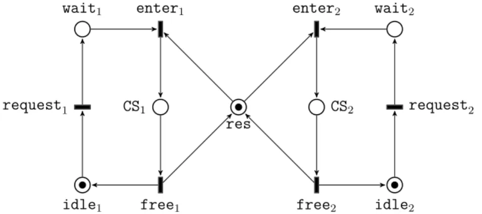
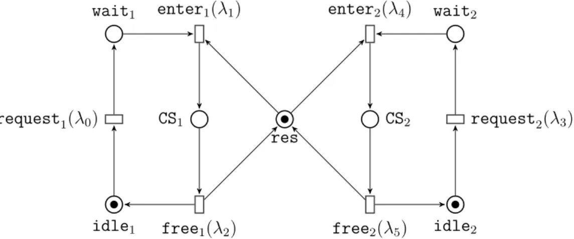
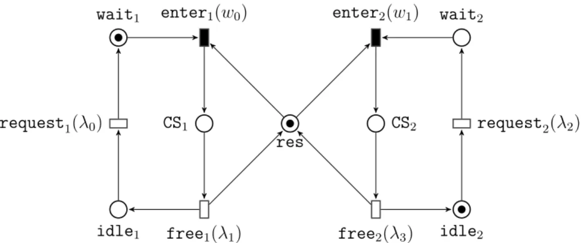
Consider PN H shown in Fig. 2.1. It models two processes p₁ and p₂ trying access a critical resource. Initial marking (i.e., state) M0 is modeled by one token in place idle1, one token in place idle2, one token in place res, and zero token in the other places. This initial state, called initial marking, is denoted by M0(CS1,CS2,idle1,idle2,res, wait1,wait2) = (0, 0, 1, 1, 1, 0, 0).

A token in places idlei, waiti and CSi means that process pi is idle, waiting to access a critical resource, and in a critical section, respectively. Transitions requesti, enteri, and freei are fired when process pi requests a critical resource, enters a critical section, and frees a critical resource, respectively.

wait1 enter1 CS1 free1 idle1 request1 res enter2 wait2 CS2 free2 idle2 request2

Figure 2.1: A PN models mutual exclusion.

2.3 Petri Net Structure

A Petri net is a bipartite directed graph that consists of places, depicted as circles, transitions, depicted as bars, and arcs connecting either place to transition or transition to place. Definition 2.1. Petri Net. A Petri net is a 4-tuple N = hP , T , F , M0iwhere

• P is a finite and non-empty set of places,

• T is a finite and non-empty set of transitions disjoint from P , • F : (P × T ) ∪ (T × P ) −→ N is a flow relation for a set of arcs, • M0 : P −→ N is an initial marking.

Some authors refer to the unmarked net N = hP , T , F i as the Petri net structure and refer to the marked net N0 _{= hP , T , F , M}

0i as the system. Furthermore, if the net marking is partially provided, then the Petri net is called a family [CDF91].

Example: Consider PN H shown in Fig. 2.1. Its formal definition is given by H = hP , T , F , M0iwhere

• P = {idle1,wait1,CS1,idle2,wait2,CS2,res},

• T = {request1,enter1,free1,request2,enter2,free2}, • F (idle1,request1) = 1, F (request1,wait1) = 1, etc.

• M0(CS1,CS2,idle1,idle2,res, wait1,wait2) = (0, 0, 1, 1, 1, 0, 0).

Definition 2.2. Preset and Postset. The inputs and outputs, called also preset and postset respectively, of places and transitions can be defined formally as follows.

• The preset of place p, denoted by •p, is given by •p = {t ∈ T |F (t, p) > 0}. • The postset of place p, denoted by p•, is given by p• = {t ∈ T |F (p, t) > 0}. • The preset of transition t, denoted by •t, is given by •t = {p ∈ P |F (p, t) > 0}. • The postset of transition t, denoted by t•, is given by t• = {p ∈ P |F (t, p) > 0}. Example: Considering PN H shown in Fig. 2.1, we have, for instance,

1. •idle1 = {free1} and idle1• = {request1}. 2. •enter1 = {wait1,res} and enter1• = {CS1}.

2.4 Dynamic Behavior of Petri Nets

Previously, we have considered the static part of PNs. In the present section, we deal with the dynamic evolution of PN marking controlled by two rules called “enabling rule” and “firing rule”. Both enabling and firing rules are specified through arc multiplicities (weights) and place markings. As for arcs, the enabling rule depends on input arcs of a transition, while the firing rule considers both input and output arcs.

Firing a transition in PN models an occurrence of its corresponding event. Before firing any transition, we check if its pre-conditions hold, in such case, the transition is said to be

enabled.

A transition t is enabled if each place in its preset contains tokens, at least, as many as the multiplicity of the arc connecting both of them.

Definition 2.3. Enabling Rule. Transition t is enabled at marking M, denoted by M[ti, iff

Example: Consider PN H shown in Fig. 2.1. Transition request1 is enabled since we have •request1 = {idle1}, M(wait1) = 1, (i.e., place idle1 contains one token), and M (wait1) ≥ F (idle1,request1).

Definition 2.4. Firing Rule. The firing of transition t enabled at marking M yields new marking M0, denoted by M[tiM0, such that

M0(p) = M (p) + F (t, p) − F (p, t), ∀ p ∈ P.

Firing transition t (i) removes from each place in its preset as many tokens as the multi-plicity of the arc connecting both of them, and produces to each place in its postset as many tokens as the multiplicity of the arc connecting both of them.

Example: Consider PN H shown in Fig. 2.1. At initial marking M0, transitions request1 and request2 are fireable. In fact, the direct arc from idle1 to transition request1 means that the pre-condition of transition request1 is place idle1. This place contains one token, that is, the pre-conditions of request1 hold, hence it can fire (i.e., the corresponding event can occur). Firing request₁ removes a token from idle1 and puts one token inside wait1, since we have an arc from request₁ to wait1, which models the post-conditions of firing request1. Similarly to transition request2 with respect to places idle2 and wait2.

PN H after firing request1 is shown in Fig. 2.2a. Firing request1 at M0 causes enabling of transition enter1 at new marking M1. Firing the latter transition at M1 leads to new marking illustrated in Fig. 2.2b. In Fig. 2.2c, transition enter2 cannot fire, since its pre-conditions are wait2 and res such that res does not contain any token which means that pre-conditions of enter2 do not hold. After firing free1 at marking depicted in Fig. 2.2c, the obtained marking is depicted in Fig. 2.2d in which enter2 becomes enabled.

Definition 2.5. Transition Sequence. A transition sequence σ = t1, t2, . . . , tn is fireable starting from marking M1 iff there exists a sequence of markings M1, M2, . . . , Mn such that Mi[tii, ∀ i ∈ {1, 2, . . . , n}.

M1[σiMn+1 denotes the firing of transition sequence σ starting from M1 and Mn+1 is reachable from M1 by firing σ.

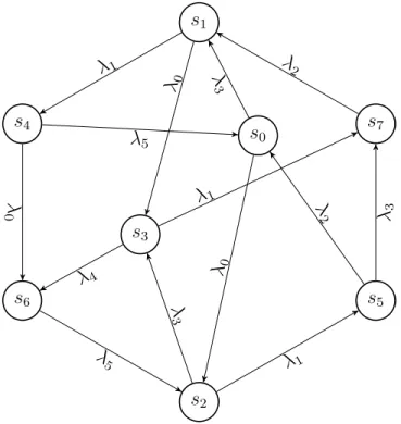
Example: Consider Table 2.1, where the initial marking is denoted by s0. Firing se-quence σ = request1,enter1,request2,free1,enter2,free2 is fireable starting from s0, since there exists a marking sequence s0, s2, s5, s7, s1, s3, such that s0[request1is2[enter1i s5[request2is7[free1is1[enter2is3[free2i.

Since PNs structure is static and firing transitions changes only the marking, which is considered as the dynamic part of PNs, the state evolution can be modeled as a graph where its nodes correspond to reachable markings, and its edges correspond to fired transitions. Such a graph is called the reachability graph. Fig. 2.3 shows the reachability graph of PN H depicted in Fig. 2.1, and their corresponding values are listed in Table 2.1.

wait1 enter1 CS1 free1 idle1 request1 res enter2 wait2 CS2 free2 idle2 request2

(a) Firing request1.

wait1 enter1 CS1 free1 idle1 request1 res enter2 wait2 CS2 free2 idle2 request2

(b) Firing request1 then enter1.

wait1 enter1 CS1 free1 idle1 request1 res enter2 wait2 CS2 free2 idle2 request2

(c) Firing request₁ enter1 request2.

wait1 enter1 CS1 free1 idle1 request1 res enter2 wait2 CS2 free2 idle2 request2 (d) Firing

request1 enter1 request2 free1. Figure 2.2: Firing transitions in PN H at M0.

Definition 2.6. Reachability Set. The Reachability set of a PN having initial marking M0, denoted by RS(M0), is defined as follows RS(M0) = {M |M0[σiM ∧ σ is a fireable sequence}.

Note that (i) σ can be empty, that is, M0 ∈ RS(M0), (ii) RS(M0) can be infinite, and (iii) an initial marking must be completely provided in order to compute the reachability set, that is, this computation is not possible neither for PN structure nor for PN family [CDF91, Mar+94].

Example: Consider PN H depicted in Fig. 2.1. Its reachability set is shown in Table 2.1, that is, RS(M0) = {s0, s1, . . . , s7}.

Definition 2.7. Reachability Graph. The Reachability graph of a PN N = hP , T , F , M0i, denoted by RG(M0) = hV , Ei, is a labeled directed graph, where

i) V = RS(M0), and

ii) E = {(Mi, t, Mj)|Mi ∈ RS(M0) ∧ Mj ∈ RS(M0) ∧ t ∈ T }.

Example: Consider PN H depicted in Fig. 2.1. Its reachability graph is shown in Fig. 2.3, that is, RG(M0) = hV , Ei where:

i) V = {s0, s1, s2, s3, s4, s5, s6, s7}, and

s1 s4 enter2 s6 request 1 s2 free 2 s5 enter1 s7 request 2 free 1 s0 request 2 request 1 free2 free 1 s3 enter2 enter1 request 1 request 2

Figure 2.3: Reachability graph of H.

CS1 CS2 idle1 idle2 res wait1 wait2

s0 0 0 1 1 1 0 0 s1 0 0 1 0 1 0 1 s2 0 0 0 1 1 1 0 s3 0 0 0 0 1 1 1 s4 0 1 1 0 0 0 0 s5 1 0 0 1 0 0 0 s6 0 1 0 0 0 1 0 s7 1 0 0 0 0 0 1

Table 2.1: Reachable markings of H.

2.5 Petri Net Analysis

Besides its modeling power, a major reason for using Petri nets is its decision power. Nu-merous analysis techniques have been developed for PNs verification. Indeed, Petri nets support the analysis of many properties and problems associated with concurrent systems [Mur89]. The properties can be analyzed either based on reachability graph, called behavioral properties, or independently from reachability graph, called structural properties.

In this section, we discuss only important properties and their analysis problems. For further reading about properties analysis, the reader is referred to [Pet81, Mur89, Mar+94, EN94, GV01, Rei12].

2.5.1 Petri Net Properties

The reachability problem for Petri nets consists of deciding if a marking M is reachable from the initial marking. It has been proven that this problem is decidable [Kos82, May84, Reu90,

p

t

p

p

t

(a) t0 is L0-live and t1 is L1-live.

p0 t3 p1 p2 t1 t2 t4

(b) t2 is L2-live, t3 is L3-live and t4 is L4-live.

Figure 2.4: Different levels of liveness.

Lam92]. The reachability problem is a central concept in Petri nets since most problems can be converted into reachability problems.

Liveness and Deadlock-freedom

A Petri net is said to be live if every transition can always fire again in the future at any reachable marking. It has been shown that the liveness problem is decidable since it is recursively equivalent to the reachability problem [AK76].

This kind of liveness is a strong property. Thus, it is relaxed to different levels of liveness [Mur89, Pet77]. A transition in a Petri net having initial marking M0 is

• L0-live (or dead) if it can never be enabled at any reachable marking.

• L1-live if it can be enabled at least once in certain firing sequence starting from M0. • L2-live if it can fire, at least, k times in certain firing sequence starting from M0, where

k is a positive integer number.

• L3-live if it appears infinitely often in certain firing sequence starting from M0. • L4-live (or live) if it is L1-live for any reachable marking from M0.

A Petri net is Lk-live if all transitions are Lk-live, such that k ∈ 0, 1, 2, 3, 4.

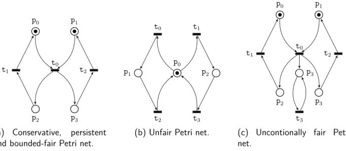
Example: Petri nets in Fig. 2.4 shows different levels of liveness, where t0 in Fig. 2.4a is dead; and transitions t1, t2, t3 and t4 in Fig. 2.4b are L1-, L2-, L3- and L4-live, respectively. Boundedness

A Petri net is bounded if its reachable set is finite. It has been proved that boundedness is decidable [KM69]. In fact, a Petri net is unbounded iff there exists a reachable marking M and transition sequence σ such that M[σiM + L, where L is a non-zero marking [EN94].

A Petri net is k-bounded if, for any reachable marking, there is at most k tokens in any place. A Petri net is safe if it is 1-bounded.

If a place in a Petri net represents a buffer, it would be interesting to verify whether this place is bounded or safe to guarantee that there will be no overflows in the buffer.

Example: PNs shown in Figs.2.4a and 2.4b are safe and non-bounded, respectively. Home state and Reversibility

A marking of a Petri net is a home state if it can be reached from all reachable markings. Authors of [Fru86, BE16] have shown that home state problem is decidable. A Petri net is said to be reversible if its initial marking is a home state.

Example: Marking M(p0,p1,p2) = (0, 0, 1)is a home state for Petri net shown in Fig. 2.4b, such that is can be reached by firing t1 once, and firing t2 until it becomes no longer enabled. Petri net in Fig. 2.1 is reversible as shown in its reachability graph depicted in Fig. 2.3. Conservation

A Petri net is said to be conservative iff the number of tokens in any reachable marking remains constant, i.e., after any transition firing the number of consumed tokens equals the number of produced tokens. This property would be useful to show that the resources (modeled by tokens) are neither created nor destroyed during the state evolution of the system.

Example: Reachable markings of Petri net depicted in Fig. 2.5a are (1, 1, 0, 0), (0, 0, 1, 1), (1, 0, 0, 1), and (0, 1, 1, 0) (the marking of p0, p1, p2 and p3).

Persistence

A Petri net is persistent if any two different transitions t1 and t2 are enable at any reachable marking M, then firing of t1 will not disable t2, and vice-versa. Authors of [Gra80, May81, Mül81] have proved that this problem is decidable.

Example: Consider Petri net shown in Fig. 2.5a. At initial marking only transition t0 is enabled. Firing this transition leads to new marking M1(p0,p1,p2,p3) = (0, 0, 1, 1) at which both transitions t1 and t2 are enabled. Firing t1 at M1 will not disable t2, and vice-versa. Fairness

There are two types of fairness: bounded-fairness and unconditional fairness. Two transitions are in a bounded-fair relation if the occurrence number of one is bounded while the other does not yet fire. A PN is bounded-fair if any two transitions are in a bounded-fair relation.

A firing sequence is unconditionally fair if it is either finite or all transitions appear infinitely often in it. A PN is unconditionally fair if all fireable sequences from its initial marking are unconditionally fair.

p0 p1

t0

p2 p3

t1 t2

(a) Conservative, persistent and bounded-fair Petri net.

t0 t1

p0

t2 t3

p1 p2

(b) Unfair Petri net.

p0 p1 t0 p2 p3 t1 t2 p3 t3

(c) Uncontionally fair Petri net.

Figure 2.5: Conservation, persistence and fairness.

Example: Consider Petri net shown in Fig. 2.5a. All firing sequences starting from initial marking are words generated from the following regular expression (t0(t1t2|t2t1))∗, i.e., are concatenations of t0 t1 t2 and/or t0 t2 t1. Thus, this Petri net is bounded-fair.

Petri net depicted in Fig. 2.5b is unfair. In fact, both transitions t0 and t2 can fire, sequentially, infinitely without any firing of neither t1 nor t3. As for PN illustrated in Fig. 2.5c, it is unconditionally fair but not bounded-fair since place p3 is an unbounded place making the occurrence number of t3, without firing other transition, unbounded as well. Mutual exclusion

There are two types of mutual exclusion dealing with the impossibility of simultaneous sub-markings or firing concurrency. Two places p and q are mutually exclusive if both of them cannot be marked at the same marking, i.e., places p and q are mutually exclusive iff ∀M ∈ RS(M0), M (p) × M (q) = 0. Two transitions are mutually exclusive if they cannot be both enabled at any reachable marking.

Example: Consider Petri net shown in Fig. 2.5b. Its reachable markings are (1, 0, 0), (0, 1, 0) and (0, 0, 1) (the values in each vector are the markings of places p0, p1 and p2, respectively). Hence, each two places in this Petri net are mutually exclusive.

Furthermore, at any reachable marking listed above, there exists one and only one fireable transition. Thus, each two transitions in this Petri net are mutually exclusive.

2.5.2 Temporal Logic

To consider a large set of properties in Petri nets, researchers have studied decidability issues using model checking [BK08].

Model-checking refers to a wide range of techniques that check whether a given property formalized by a temporal logic is verified by a given system modeled, often, by a transition system. The model checker confirms that either the system satisfies the property or violates it. In the latter case, a counter-example is provided.

Among the properties that can be checked by model checking, there are two important types of properties, namely, the liveness and safety properties [GV01]. Roughly speaking, a liveness property (eventually) must be satisfied in the future by all future executions, i.e., “good things” do happen. For instance, if a process asks for a critical resource, it will access to it in the future. A safety property (always) must be satisfied in each reachable state in the future, i.e., “bad things” do not happen. For instance, a critical resource will never be used by two processes or more at the same time. It has been shown in [AS87] that any property can be decomposed as a conjunction of safety and liveness properties.

Aforementioned, usually model checker requires formalizing properties as formulae of temporal logic and describing systems as transition systems. In the following, we present briefly transition systems and temporal logic.

Definition 2.8. Transition System. A transition system T S is a tuple hS, T , E, I, A, Li, where:

• S is a set of states and T is a set of actions, • E ⊆ S × T × S is a transition relation on S, • I ⊆ S is a set of initial states,

• A is a set of atomic propositions,

• L : S −→ 2A is a labeling function that assigns truth value to atomic propositions at each state, that is, a ∈ A is true at s ∈ S iff a ∈ L(s).

In PNs context, S, T and E are obtained from the reachability graph, I contains a single initial marking, and the atomic propositions are conditions on place markings.

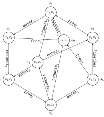
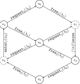
Example: Consider transition system T S depicted in Fig. 2.6 of Petri net H shown in Fig.2.1. T S is defined as follows. T S = hS, T , E, I, A, Li, where:

• S is the set of reachable states of H, that is S = {s0, s1, s2, s3, s4, s5, s6, s7}, • T = {request1,request2,enter1,enter2,free1,free2},

I1,W2 s1 I1,C2 s4 enter 2 W1,C2 s6 request 1 W1,I2 s2 free 2 C1,I2 s5 enter1 C1,W2 s7 request 2 free 1 I1,I2 s0 request 2 request 1 free2 free 1 W1,W2 s3 enter 2 enter1 request 1 request 2

Figure 2.6: Transition system of H shown in Fig. 2.1, where Ii, Wi and Ci denote (idlei = 1), (waiti = 1) and (CSi = 1) for each i ∈ {1, 2}, respectively.

• E = {(s0,request2, s1), (s0,request1, s2), (s1,enter2, s4), (s1,request1, s3), . . . }, • I = {s0},

• A = {(idle1 = 1), (idle2 = 1), (wait1 = 1), (wait2 = 1), (CS1 = 1), (CS2 = 1)}, such that (idle1 = 1) means idle1 is marked by one token. Similarly to the other places, • L is the labeling function such that L(s0) = {(idle1 = 1), (idle2 = 1)}, L(s1) =

{(idle1 = 1), (wait2 = 1)}, L(s2) = {(wait1 = 1), (idle2 = 1)}, etc.

Definition 2.9. Finite Path, Maximal Path, and Path. A finite path is a state sequence s0s1. . . sn, where ∃ (si−1, t, si) ∈ E, such that t ∈ T , for all i ∈ {1, 2, . . . , n}. A maximal path π of a transition system with no terminal state is an infinite sequence of states s0s1s2. . ., such that ∀ i, ∃ t ∈ T , (si, t, si+1) ∈ E. A maximal path π = s0 s1 s2. . . is a path, if s0 ∈ I. Example: Consider transition system T S depicted in Fig. 2.6. s0s2s5s7 is a finite path, s2s5s7s1s4s0 s1. . . is a maximal path, and s0s2s5s7s1s4s0. . . is a path.

Definition 2.10. Trace. The trace of a maximal path π = s0s1s2. . . is defined as trace(π) = L(s0)L(s1)L(s2) . . .. That is, the trace registers the valid propositions in each state of π. Example: The trace of s0s2s5s7s1s4s0. . . is {I1,I2}{W1,I2}{C1,I2}{C1,W2}{I1,W2}{I1,C2} {I1,I2} . . ..

As for temporal logics, there are two categories, namely, linear time logic (LTL) and branching time logic (CTL). In this dissertation, we will restrict our attention to the linear temporal logic. A comprehensive formal description of model checking can be found in [BK08].

Definition 2.11. LTL Formula. An LTL formula is inductively defined as follows. Φ ::=true | a | ¬Φ | Φ1∨ Φ2 | XΦ | Φ1 U Φ2

where a ∈ A is an atomic proposition.

Example: All the following formulae are LTL formulae. • Φ1 ::= (CS1 = 1),

• Φ2 ::= ¬(CS1 = 1) ∨ ¬(CS1 = 1), • Φ3 ::=X(¬(CS1 = 1) ∨ ¬(CS1 = 1)), • Φ4 ::= (wait2 = 1)U(CS2 = 1).

Informally, formula XΦ holds for a maximal path π if its second state satisfies Φ. For instance, consider path π0 = s0s2s5s7s1s4s0. . .. Formula Φ3 holds for π0 since (¬(CS1 = 1) ∨ ¬(CS1 = 1)) is satisfied in s2.

As for formula Φ1UΦ2, it holds for a maximal path π if there exists a state s satisfies Φ2, such that each prior state thereof satisfies Φ1. For instance, consider maximal path π1 = s7s1s4s0. . .. Formula Φ4 holds for π1, since formula (wait2 = 1) holds for s7 and s1; and formula (CS2 = 1)is satisfied in s4. As for maximal path π2 = s7s1s3s7s1s3s7. . ., formula Φ4 does not hold.

Operators eventually (denoted by F) and always (denoted by G) can be expressed via operator U, such that (FΦ ≡ trueUΦ) and (GΦ ≡ ¬F¬Φ).

2.5.3 Analysis Methods

In literature, Petri net analysis methods can be categorized as: enumeration or net-driven. The first category consists on the computation of the reachability graph (totally or par-tially). If the reachability graph is finite, it can be used for a proof system or for decision procedures, where the most important properties are decidable. On the other hand, we can use the coverability tree for unbounded systems, however, important properties such as liveness and reachability are not decidable [Pet81]. Basically, enumeration based methods are applicable to any Petri net class, however due to computational complexity, their use is limited to small nets [Mur89].

To overcome state space explosion problem, net-driven approaches reason on the net structure to extract useful information about the net behavior.

Two different approaches are: structure theory and net transformations. The former is based on graph theory and/or linear algebra. The latter transforms Petri net to another one (typically by reduction) while preserving the properties to be analyzed. The resulting models are expected to be easier to analyze [GV01].

Analysis by transformation transforms a net system S into a net system S0 preserving a set of properties Π in such a way that verifying set Π in S0 becomes easier than in S such that S0 may belong to a Petri net subclass for which state enumeration can be avoided.

A special class of transformation methods is reduction methods in which a net system S is transformed into a net system S0 (eventually using a reduction sequence) in such a way that S0 is smaller than S preserving a set of properties Π of S.

In structural analysis techniques, the net behavior is reasoned from its structure, and its initial marking is considered as a parameter. We can find two subcategories of structural analysis:

1. Linear algebra: Using matrix equations, they allow fast verification without the neces-sity of enumeration in certain cases.

2. Graph-based techniques: They are effective in analyzing some subclasses of Petri nets. Although net-driven techniques are powerful, in many cases they are applicable only to special subclasses of Petri nets [Mur89]. For further information about these analysis techniques, the reader is referred to [Pet81, Mur89, GV01].

2.6 Stochastic Petri Nets

In this section, we present a class of Petri net enriched by temporal concepts, namely stochas-tic Petri nets (SPNs). Indeed, Petri nets, in their basic definition, do not involve any concept of time quantification. The notion of time is abstract in basic Petri nets, i.e., only logical relationships in terms of time such as transition t1 fires before transition t2, transition t3 fires

after transition t4, etc. are allowed. Thus, performance evaluation of systems using basic

Petri nets is not possible.

On the other hand, the time concept is viral in certain real applications whose efficiency is a crucial aspect. Hence, time-augmented Petri nets are introduced. In general, there are two possible ways to do this [BK02]:

• Timed places Petri nets (TPPNs): In this class of Petri nets, tokens fired onto a place p are unavailable to all its output transitions for a certain time. Once this time has elapsed the tokens become available.

• Timed transitions Petri nets (TTPNs): In this class of Petri nets, once a transition becomes enabled it does not fire immediately, instead, it fires after a certain time. Time-augmented Petri nets are classified also depending upon time nature. In fact, if time is deterministic, then such Petri nets are called “timed Petri nets”. On the other hand, if the firing time is a random variable following a certain distribution law, then they are called “stochastic Petri nets”. Different families of stochastic Petri nets can be defined based on their distribution laws of the firing time.

Moreover, the nature of stochastic Petri nets depends also on other firing characteristics [Mic01], namely:

Selection policy: Given a set of enabled transitions at a certain marking, there are two policies concerned with how tokens are reserved until the transition firing:

1. Preselection policy. First, (i) an enabled transition reserves all tokens it needs so that these tokens are not available for other transitions. Then, (ii) it waits for its firing time to elapse. Finally, (iii) it fires immediately according to the firing rule of Petri nets. 2. Race policy. First, (i) an enabled transition waits until its firing time interval has

elapsed. Then, (ii) it fires immediately according to the firing rule of Petri nets provided it is still enabled at that time, i.e., the required tokens are not already consumed by another transition.

Service policy: Given an enabled transition at a certain marking at which it can fire k times, there are three policies concerned with how many times should the transition be fired when its firing time has elapsed:

1. Single-server. One single firing is performed. It means that transition can only offer one service at time,

2. Infinite-server. k firings are performed. It means that transition can ensure any number of simultaneous services,

3. Multiple-server. Min(k, deg(t)) firings are performed. It means that transition t can ensure deg(t) simultaneous services at maximum.

Memory policy: Assume that each timed transition is associated with a timer. When a timed transition becomes enabled, its corresponding times is set to an initial value and then starts to decrement. When the timer reaches the value zero, the corresponding transition fires. Given a set of enabled transitions at a certain marking, there are three policies concerned with how should firing a transition influence the timers of the other transitions:

1. Resampling. At each firing, the timers of all the timed transitions are discarded (restart mechanism),