Refined Instrumental Variable method for non-linear dynamic identification of robots

HAL Id: hal-00520261

https://hal.archives-ouvertes.fr/hal-00520261

Preprint submitted on 22 Sep 2010

HAL is a multi-disciplinary open access

archive for the deposit and dissemination of

sci-entific research documents, whether they are

pub-lished or not. The documents may come from

teaching and research institutions in France or

abroad, or from public or private research centers.

L’archive ouverte pluridisciplinaire HAL, est

destinée au dépôt et à la diffusion de documents

scientifiques de niveau recherche, publiés ou non,

émanant des établissements d’enseignement et de

recherche français ou étrangers, des laboratoires

publics ou privés.

Refined Instrumental Variable method for non-linear

dynamic identification of robots

Alexandre Janot, Pierre-Olivier Vandanjon, Maxime Gautier

To cite this version:

Alexandre Janot, Pierre-Olivier Vandanjon, Maxime Gautier. Refined Instrumental Variable method

for non-linear dynamic identification of robots. 2010. �hal-00520261�

Refined Instrumental Variable method for non-linear dynamic

identification of robots

A.

Janot

a

, P-O Vandanjon

b

, M Gautier

c

a _{Haption SA, Laval, France, [email protected]} b

Laboratoire Central des Ponts et Chaussées, Nantes, France, [email protected]

c

Institut de Recherche en Communication et Cybernétique de Nantes, France, [email protected]

Abstract

The identification of the dynamic parameters of robot is based on the use of the inverse dynamic identification model which is linear with respect to the parameters. This model is sampled while the robot is tracking “exciting” trajectories, in order to get an over determined linear system. The linear least squares solution of this system calculates the estimated parameters. The efficiency of this method has been proved through the experimental identification of a lot of prototypes and industrial robots. However, this method needs joint torque and position measurements and the estimation of the joint velocities and accelerations through the bandpass filtering of the joint position at high sample rate. So, the observation matrix is noisy. Moreover identification process takes place when the robot is controlled by feedback. These violations of assumption imply that the LS estimator is not consistent. This paper focuses on the Refined Instrumental Variable (RIV) approach to over-come this problem of noisy observation matrix. This technique is applied to a 2 degrees of freedom (DOF) prototype devel-oped by the IRCCyN Robotic team.

Key words: Identification algorithms, Least-squares methods, Robot dynamics

1. Introduction

The usual identification method based on the inverse dynamic model (IDM) and LS technique has been success-fully applied to identify inertial and friction parameters of a lot of prototypes, industrial robots and has been ex-tended to cars, worksite engine, human being and haptic interfaces (Atkeson, An, et Hollerbach 1986)(Swevers et

al. 1997)(Khosla et Kanade 1985)(Kozłowski

1998)(Raucent et al. 1992)(Gautier 1986)(Restrepo et Gau-tier 1995)(GauGau-tier 1997)(Venture et al. 2006) (C-E Le-maire et al. 2006)(Janot et al. 2007) among others. At any case, a derivative bandpass data filtering is required to cal-culate the joint velocities and accelerations. Moreover identification process is carried out with a feedback con-trolled robot. These conditions may lead to a violation of statistical independence between the residual and the ob-servation matrix which implies that the LS solution is not consistent. To overcome this problem of noisy observation matrix, several methods have been proposed in the past: Extended Kalman Filtering, total least-squares, Instrumen-tal Variable method.

We show in (Gautier et Poignet 2001) that Extended Kalman Filtering is more complicated without improve-ments of results.

As far as total least squares are concerned, we used them in order to identify simultaneously dynamic and drive gain parameters (Gautier, P.O. Vandanjon, et Presse 1994). However, we did not succeed in applying this method to take into account the feedback which correlates the noise.

Instrumental Variable method was already applied in robotics (Puthenpura et Sinha 1986). This method was used in order to identify a SISO system linear with respect to the state in an open loop configuration for each axis of an industrial robot. In this paper, the IV is applied for a dynamic model of a robot non linear with respect to the state and in closed loop configuration.

Recently, the Instrumental Variable (IV) approach was renewed in the context of closed loop linear continuous system.

This method is particularly interesting because of its simplicity. Indeed, no noise model identification is needed and the IV estimator is consistent even if the noise is col-ored (Young et Jakeman 1979), (Söderström et Stoica 1989). However, this technique was generally applied to discrete system linear with respect to the state which is not the case in robotics. The choice of the instrument variable depends on the context. Moreover, the method was de-signed in open loop system. Progressively, algorithms suit-able to our context, i.e. continuous time and closed loop system, have emerged. In particular, the so-called SRIVC

algorithm (Simplified Refined Instrumental Variable Con-tinuous-time) for open loop system, based on an auxiliary model as instrument variable, is a good candidate to our problem (Young 2006). Very recently, this last algorithm was modified in order to take into account closed loop sys-tem (Gilson et al. 2006)(Young, Garnier, et Gilson 2009) but still in the frame of system linear with respect to the state. This technique is implemented in the MATLAB CONTSID toolbox developed by the CRAN team (Garnier, Gilson, et Cervellin 2006).

A derivation of this IV method was first successfully applied on a 1 DOF haptic device (P-O. Vandanjon et al. 2007). This derivation is based on the use of both the in-verse dynamic model (IDM) and the direct dynamic model (DDM). The robustness to data filtering and to the initiali-zation as the calculation of the optimal solution were pre-sented in (Janot, P-O. Vandanjon, et Gautier 2009). How-ever, the consistence of the estimation (like statistical rules), the convergence of the purposed algorithm and the robustness to control laws were not introduced. This paper deals with these issues and the IV method is carried out on a 2 DOF prototype robot developed by the IRCCyN ro-botic team. This direct drive prototype is very well suited to our purpose because it emphasizes non linear coupling contrary to industrial robots with high gear ratio.

The paper is organized as follows: section 2 reviews the usual identification technique of the dynamic parameters of the robot. Section 3 presents the Instrumental Variable techniques. The experimental results are given in section 4. Finally, section 5 is the conclusion

2. IDIM

The inverse dynamic model (IDM) of a rigid robot com-posed of n moving links calculates the motor torque vector

idm

τ , as a function of the generalized coordinates and their

derivatives. It can be obtained from the Newton-Euler or the Lagrangian equations, (W. Khalil et Dombre 2002), (Featherstone et Orin 2008). It is given by the following relation:

= ( ) + ( , )

idm

τ M q q&& N q q& (1)

Where, q , q& and q&& are respectively the

( )

n 1x vectors of generalized joint positions, velocities and accelerations,

( )

M q is the

( )

n nx robot inertia matrix, and N q q( , )& is the

( )

n 1x vector of centrifugal, Coriolis, gravitational and friction forces/torques.

The choice of the modified Denavit and Hartenberg frames attached to each link allows to obtain a dynamic model lin-ear in relation to a set of standard dynamic parameters, χ_st (Gautier 1986), (Gautier et W. Khalil 1990):

(

)

idm st st

τ =IDM q,q,q χ& && (2) Where IDM_st

(

q,q,q& &&

)

, is the

(

n Nx _s

)

jacobian matrix of

idm

τ , with respect to the

(

Nsx1

)

vector χst, of the stan-dard parameters given by:

T T T T ... 1 2 n st st st st χ ₌_χ χ χ _{ (3)} With: χsj = [XXj XYj XZj YYj YZj ZZj MXj MYj MZj Mj Iaj Fvj Fcj τoffj]T, where:

o XX , XY , XZ , YY , YZ , ZZ , are the six components _{j j j j j j}

of the inertia matrix, j j

J , of link j at the origin of frame j,

o MX , MY , MZ , are the components of the first mo-_{j j j}

ments,j j

MS , of link j,

o M is the mass of link j, _j

o Ia , is a total inertia moment for rotor and gears of ac-_j

tuator j.

o Fv , _j Fc , are the viscous and Coulomb friction pa-_j

rameters of joint j.

o

j

off Fsj tj

τ =Of +Of , is an offset parameter where Of_Fsj is

the dissymmetry of the Coulomb friction with respect to the sign of the velocity and Of is due to the current _tj amplifier offset which supplies the motor.

o N_s = ×14 n, is the number of standard parameters. The base parameters are the minimum number of dy-namic parameters from which the dydy-namic model can be calculated. They are obtained from the standard inertial parameters by eliminating those which have no effect on the dynamic model, and by regrouping some others by means of linear relations. They can be determined using simple closed-form rules (Gautier et W. Khalil 1990) or using a numerical method based on the QR decomposition (Gautier 1991).

The minimal inverse dynamic model can be written as:

(

)

idm

τ =IDM q,q,q& && χ (4)

Where:

(

)

IDM q,q,q& && , is the

( )

n b matrix of the minimal set of x

basis functions of the rigid body dynamics, (5)

χ , is the

( )

b 1 vector of the b base parameters. x (6) Because of perturbations due to noise measurement and modeling errors, the actual force/torque τ differs from

idm

τ , by an error e , such that:

(

)

idm

τ e IDM q,q,q χ e

τ = + = & && + (7)

Equation (7) gives the Inverse Dynamic Identification Model (IDIM).

We consider the off-line identification of the base

dy-namic parameters χ, given measured or estimated off-line

data for τ and

(

q, q, q & &&

)

, collected while the robot is tracking some planned trajectories.

Usually, the signals available from the robot controller are the joint position measurement and the

( )

n 1 control x signal vector v_τ, calculated according to the control law.

Then

(

q, q, q & &&

)

in (7) are estimated with

(

ˆq, q, q & &&ˆ ˆ

)

respec-tively, obtained by bandpass filtering the measure of q (Gautier 1997). The derivatives are off-line calculated without phase shift, using a central difference algorithm of the lowpass filtered position ˆq . The filtered position ˆq is off-line calculated with a non causal zero-phase digital

fil-ter by processing the input data q , through a lowpass

But-terworth filter in both the forward and reverse direction, using the filtfilt procedure from Matlab.

The control signal v_τ, is connected to the input current reference of the current closed-loop of the amplifiers which supplies the motors. Assuming that the current closed-loop has a large bandwidth, greater than 500Hz, its transfer function is equal to its static gain, K , in the fre-_c quency range (less than 10Hz) of the rigid robot dynamics. Then, the actual force/torque τ, is calculated with the rela-tion:

g v_{τ τ}

τ = (8)

where:

g_τ, is the

( )

nxn diagonal matrix of the drive gains, with:

r c

g_τ =K K K_τ (9)

where:

o K , is the _r

( )

nxn gear ratios diagonal matrix of the joint

drive chains (q&_m =K q_r& , with &q_m, the velocity on the motor side),

o K , is the _c

( )

nxn static gains diagonal matrix of the

cur-rent amplifiers,

o K_τ, is the

( )

nxn diagonal matrix of the electromagnetic motor torque constants.

oThose parameters have a priori values, given by manu-facturers, which can be checked with special tests (Restrepo et Gautier 1995).

The inverse dynamic identification model (IDIM) (7) is

calculated at a frequency measurement f , using samples _m

of

(

ˆq, q, q & &&ˆ ˆ

)

to calculate IDM q,q,q

( )

ˆ & &&ˆ ˆ and samples of v_τ to calculate τ with (8), at different times t , _k k=1,...,n_m, while the robot is tracking a reference trajectory

(

q ,q ,qr & &&r r

)

, during the time length Tobs, of the trajectory. The equations of each joint are regrouped together on all the trajectory to get an over-determined linear system such that:

( )

( )

fm fm ˆ ˆ ˆ fm Y τ =W q,q,q& && χ+ρ (10) With:

( )

m 1 fm j 1 j fm fm n fm j n Y ( t ) Y τ ... , Y ... Y ( t ) τ τ         =  =          (11)

( )

( ( ) ( ) ( )) ( ( ) ( ) ( ) m m m 1 j fm 1 1 1 j fm fm n _j fm _{n n n} ˆ ˆ ˆ W IDM q t ,q t ,q t ˆ ˆ ˆ W q,q,q ... , W ... ˆ ˆ W IDM q tˆ ,q t ,q t         =_{ } =        _ _ & && & && & && (12) where: ( ( ) ( ) ( )) j k ˆ k ˆ k ˆ

IDM q t ,q t ,q t& && , is the jth row of the

( )

n b re-x gressor matrix IDM q t ,q t ,q t( ( ) ( ) ( ))ˆ _k &ˆ _k &&ˆ _k , (5).

j fm

Y and j

fm

W , represent the n equations of joint j , _m

*

m obs m

n =T f , is the number of sample measurements.

The notation W_fm

(

IDM q,q,q

( )

ˆ & &&ˆ ˆ

)

=W_fm

( )

q,q,qˆ& &&ˆ ˆ will be used also to recall that W_fm, is calculated with a sampling of IDM q,q,q

( )

ˆ & &&ˆ ˆ .

In order to eliminate high frequency force/torque ripple in τ, and to window the identification frequency range into the model dynamics, a parallel decimation procedure low-pass filters in parallel Y_fm and each column of W_fm and resamples them at a lower rate, keeping one sample over

d

n . This parallel decimation can be carried out with the Matlab decimate function, where the lowpass filter cut-off frequency is equal to 0.8×f_m/(2×n_d).

After the data acquisition procedure and the parallel de-cimation of (10), we obtain the over determined linear sys-tem:

( )

( )

_ˆ ˆ ˆ

Y τ =W q,q,q χ& && +ρ (13) where:

o Y τ

( )

, is the ( rx1) vector of measurements, built from the actual force/torque τ ,

oW q,q,q

( )

ˆ & &&ˆ ˆ , is the ( r b )x observation matrix, built from the estimated values

( )

ˆq,q,q& &&ˆ ˆ of

(

q, q, q & &&

)

.

o ρ, is the ( rx1) vector of errors.

o r=n* n / n_{m d} , is the number of rows in (13).

In Y and W, the equations of each joint are grouped together such that:

, 1 1 n n Y W Y ... W ... Y W         =  =          (14) where j Y and j

W represent the n / n_{m d} equations of joint j .

squared 2-norm ρ2 of the vector of errors.

Using the base parameters and tracking “exciting” ref-erence trajectories (Gautier et W. Khalil 1992) allow to get

a full rank and well conditioned matrix W. The LS

solu-tion ˆχ is given by:

(

)

(

_T 1 _T

)

ˆχ= W W − W Y =W Y+ (15)

It is computed using the QR factorization of W . Stan-dard deviations

i

ˆ

χ

σ , are estimated using classical results

from statistics under the assumptions that W is a

determi-nistic matrix, thanks to the data filtering procedure de-scribed above, and ρ , is a zero-mean additive independent Gaussian noise, with a covariance matrix C , such that: _ρρ

T 2

ρρ ( ) σρ r

C =E ρρ = I (16)

where E is the expectation operator and I , the _r

( )

r r x identity matrix.

An unbiased estimation of the standard deviation σ_ρ is:

2 2

ρ

σ (r b )

ˆ = Y−Wχˆ − (17)

The covariance matrix of the estimation error is given by: T 2 T 1 χχ [( )( ) ] σρ( ) ˆ ˆ ˆ ˆ ˆ C =E χ−χ χ−χ = W W − (18) i 2 χ χχ

σ_ˆ =C (_{ˆ ˆ} i,i) is the ith diagonal coefficient of C . The _χχˆˆ relative standard deviation

ri χ %σˆ is given by: ri i χ χ i %σˆ =100σˆ χˆ , for χˆi ≠ 0 (19)

The OLS can be improved by taking into account differ-ent standard deviations on joint j equations errors (Gautier 1997). Each equation of joint j in (13), (14), is weighted with the inverse of the standard deviation of the error calculated from OLS solution of the equations of joint j , given by:

( )

(

( )

)

j j j j

j

ˆ ˆ ˆ

Y τ =W IDM q,q,q& && χ+ρ (20)

This weighting operation normalizes the errors in (13) and gives the weighted LS (WLS) estimation of the pa-rameters.

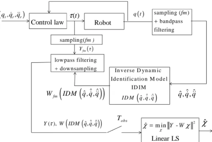
This identification method is illustrated in Fig. 1. The calculation of the velocities and accelerations are re-quired using well tuned bandpass filtering of the joint posi-tion (Gautier 1997).

One of the numerous validations of the identification is to simulate, a posteriori, the direct dynamic model (DDM) given by (10) and to compare the simulated trajectories with real trajectories when the torques are the same. These comparisons have to be done on trajectories which were not used for the identification process.

(

)

1 q=M ( q )− τ - N( q, q ) && & (21) Robot

(

)

In v erse D yn a m ic Id e n tifica tio n M o d e l ID IM ˆ ˆ ˆ

ID M q ,q , q& && q q qˆ, ,ˆ ˆ& &&

(

)

(

)

fm ˆ ˆ ˆ

W IDM q ,q ,q& &&

Linear LS 2 ˆ m inY-W χ χ= χ

(

)

(

ˆ ˆ ˆ

)

( ), , ,

Yτ W IDM q q q& &&

( ) q t ( )t τ Control law ˆ χ (q ,q ,qr& &&r r) obs T sampling ( ) bandpass filtering fm + lowpass filtering + downsampling sampling(fm ) ( ) fm Y τ

Fig. 1: IDIM LS identification scheme.

3. Instrumental variable technique

3.1. Theoretical approach

From a theoretical point of view, the statistical assump-tions for efficient LS estimation are violated in practical applications. In the equation (13), the observation matrix W is built from the measured joint positions q and from , which are numerically computed from q ,q ,q& && . Therefore the observation matrix is noisy. Moreover identification is carried out in closed-loop control. These violations of

as-sumption imply that the LS estimator, ˆχ, may be non

con-sistent. Indeed, from (13) , it comes:

T T T T

ev ˆ

W Y=W Wχ+W ρ =W W χ (22)

With ρ_ev is the vector of errors (errors in variable) when

W is corrupted by noiseW =W_nf −∆W

ev

ρ =∆ χW +ρ (23)

Thanks to the Slutsky’s theorem, it is obtained:

1

T T

1 1

plim plim _{m m} plim _{m evm}

m m m ˆχ χ W W W ρ m m − →∞ →∞ →∞     = +         (24) With: m plim

→∞is the convergence in probability,

m is the number of repetition of W and ρ_ev, m

W (resp. ρ_evm ) is the concatenation of W (resp. ρ_ev).

Under the classical assumptions:

(

T

)

plim T E m m m 1 W W W W m →∞   =     is positive definite (25) plim _mT _evm E T _ev m 1 W ρ (W ρ ) m →∞   =     exists (26)

As ρ_ev depends on the observation matrix W according to

(23), E(W ρ )T ≠0. Therefore, the estimator is not consis-tent.

Instrumental Variable method deals with this problem of noisy observation matrix (called error in variable in the sta-tistical frame) and can be stasta-tistically optimal (Davidson et Mackinnon 1993) (Young et Jakeman 1979). The Instru-mental Variable Method proposes a consistent estimator by building the instrument matrix V such as (22) becomes:

T T T T

V

ev ˆ

V Y=V Wχ V ρ+ =V Wχ (27)

The instrumental variable solution, ˆχ , is the solution of _V (27):

( )

T T

V

1

ˆχ = V W − V Y (28)

In the following V is calculated as a function of χˆ_V . That defines an iterative procedure such as:

( )

T T

Vk 1 k k

1

ˆχ ₊ = V W − V Y (29)

where : V_k =V χ

( )

ˆ_Vk

This needs for

( )

T

k

V W to be a regular matrix. Assuming:

plim _k,mT _m m 1 V W m →∞    

 is non singular and, (30)

plim k,mT evm E kT ev m 1 V ρ (V ρ ) 0 m →∞   = =     (31)

With V_{k ,m} is the concatenation of V _k

for any k, χˆ_Vk converges to χ with m. Indeed, with the Slutsky’s theorem, we obtain:

1

T T

Vk k,m k,m

1 1

plim plim _m plim _evm

m m m ˆχ χ V W V ρ m m − →∞ →∞ →∞     = +         (32)

And with (30) and (31), it comes:

Vk plim m ˆχ χ →∞ = (33) Then the IV estimator is consistent.

3.2. Calculation of the instrumental matrix

The main problem is to find an instrument matrix V. A usual solution is to build an observation matrix from simu-lated data instead of measured data. These simusimu-lated data (called also instruments) are the outputs of an auxiliary model (Young et Jakeman 1979) which is an approxima-tion of the noise-free model of the process to be identified. We chose the Direct Dynamic Model of the robot (DDM) given by (21) to be this auxiliary model.

The IV method adapted for dynamic identification of robots can be resumed by the following algorithm illus-trated

Fig. 2:

• The algorithm is initialized with any the values ac-cording to the subsection 3.4.

• At each step of the iterative algorithm, q ,q ,q_S & &&_{S S}are calculated by simulation of the closed loop robot tracking exciting trajectories using the DDM with the parameters identified at the previous step. W is obtained as a sam-_S

pling of IDIM, ID_S

(

q ,q ,q_S & &&_{S S}

)

, and we choose the in-strument matrix as:

( )

Vk

(

S S S Vk

)

k ˆ S ˆ

V χ =W q ,q ,q , χ& && ₍₂₂₎

( )

Y τ is calculated from the sampling and filtering of the

measurements of τ , and W q,q,q

(

& &&

)

is calculated through IDIM using the sampling and filtering of q .

• χˆ_Vk+1 is given by (29) which is the LS solution of

(27),

• The algorithm stops when the relative error decreases under a tolerance, ideally chosen to be a small number): with the estimation error:

k SˆVk

ε = −Y W χ

Fig. 2 : IV identification procedure

3.3. Calculation of the solution

Suitable solutions consist in using orthogonal projection such as QR decomposition. In this case, we have:

W W W =Q R , V V V =Q R

.

With: V

Q and Q are orthogonal matrices which are projectors _W

on the vectorial subspace spanned by the columns of V and W.

V

R and R are upper triangular matrices. _W

Considering only the b base parameters to be identified, we check we have at each iteration:

rank(RW) = rank(QW) = rank(RV) = rank(QV) = b.

This relation guarantees that the matrix VTW is invertible. Then, equation (27) becomes:

k 1 k k ε ε ε α + − _≤ robot S S S,q ,q

q & && τ q Control Law Control Law S τ

( )

(

(

)

)

V Vkk ˆ DDM( ) S S S S S M q q τ N q ,q χχχχ = − && & Band pass filter ˆ ˆ ˆq,q,q& &&

( )

_ˆˆ ˆ IDM q,q,q& &&

(

)

s a m p l in g + / /f i lt e r i n g ˆ ˆ ˆ I D M → W q ,q ,q & && ( ) Vk ID IM ˆ

τ_S=ID_S q ,q ,q_S& &&_{S S} χ

(

)

S_sampling S S S S

IDM → W q ,q ,q =V & && _k

obs T sampling+filtering τ → Y obs T T k k Vk+1 T ˆ V Y V W=

χ

obs T r r r q q q           & &&

Actual closed loop robot

T T T T

V

V V W W V ev V W Wˆ

Q Y=Q Q R χ+Q ρ =Q Q R χ (34)

V

ˆχ is the LS solution of the last equations.

Compared with LS regressions, the IV method needs two QR decompositions.

3.4. Initialization of the algorithm

Another problem is to choose the initial values ˆχ . 0 We can use CAD values, or identified values with the IDIM method, but we show that there is no need at all of a priori values.

We propose an algorithm not sensitive to the initial condi-tions, which assumes that the condition

(

qddm( χ ),qˆk &ddm( χ ),qˆk &&ddm( χ )ˆk

) (

q,q,q& &&

)

(35) is satisfied at any iteration k , and especially for k =0. This is possible by taking the same control law structure for the actual robot and for the simulated one with the same performances given by the bandwidth, the stability margin or the closed-loop poles. Because the simulated ro-bot parameters ˆχ , change at each iteration k , the gains k of the simulated control law must be updated according to

k

ˆχ .

For example, let us consider a PD control law for each joint j . The inverse dynamic model IDM (1) for the joint j , can be written as a decoupled double integrator per-turbed by a coupling force/torque, such that:

= ( ) + ( , ) = ( ) ( ) + ( , )= ( ) j n j idm j ,i i j i 1 n j , j j j ,i i j j , j j j i j τ τ M q q N q q M q q M q q N q q M q q p = ≠ = + −

∑

∑

&& &

&& && & &&

(36)

where p is considered as a perturbation given by: _j

( ) ( , ) n j j ,i i j i j p M q q N q q ≠ = −

∑

&& − & (37) ( ) j ,i

M q , which depends on q , is approximated by a

constant inertia moment J , given by: _j

(

( )

)

j j j j a j , j j a q J =ZZ +I +max M q −ZZ −I (38) j

J , is the maximum value, with respect to q , of the in-ertia moment around joint z axis. This gives the smallest _j damping value and the smallest stability margin of the closed-loop second order transfer function (42), while q varies.

It can be calculated from a priori CAD values of inertial parameters and must be taken at least as

j

j a

ZZ +I .

The joint j dynamic model is approximated by a dou-ble integrator, where p , is a perturbation, as following: _j

(

)

(

)

( ) j j j j j j , j j 1 1 q τ p τ p M q J = + + && (39)

Let us consider the joint j PD control of the actual robot which is illustrated Fig. 3:

+ - +- j a gτ j r q j a v k a1 j J 1 s 1 s ++ j a p k j p j v_τ τj q&&j q&j qj

Fig. 3: Joint PD control of the actual robot.

The control input calculated by the robot controller is given by:

(

)

j j j j j a a a p v r j v j v_τ = k k q −q − k q& (40) j

v_τ , is the current reference of the current amplifiers which supplies the motor.

The joint j , force/torque is given by:

j j a j g vτ τ τ = (41) where: j a

gτ , is the actual drive gain, calculated with the actual

parameters in (9). a

j

J , is the actual value of J_j.

• In order to tune the tracking performances of the

reference position

j

r

q , the transfer function rj

j q q is calcu-lated with p_j=0: =0 =0 j j j j j j j j j j a 2 r j p a a a a v p p j j 2 a r j p a 2 a nj nj q ₁ H q J s ₁ s 1 g k k k q 1 H q _s 2 s 1 τ ζ ω ω     =_{ } =   _{+ +}     =_{ } =   _{+ +} (42) where: a nj

ω , is the actual natural frequency which characterizes

the closed-loop bandwidth, a

j

ζ , is the actual damping coefficient which

character-izes the closed-loop stability margin, with:

j i i a a a a nj p v a j g k k J τ ω = , 1 i j i a a v a j a a p j g k 2 k J τ ζ = (43) Then it comes: 2 j a nj a p a j k ω ζ = , j j a j a a a v j nj a J k 2 g_τ ζ ω = (44)

The closed-loop performances are chosen with the desired 2 poles of a second order transfer function characterized by, d nj ω , d j ζ , where: d nj

ω , is the desired natural frequency, d

j

ζ , is the desired damping coefficient.

Because the actual values are unknown, the gains are calculated from (44), where the unknown actual values,

a nj ω , a j ζ , a j J , j a i

g , are replaced respectively by their desired values, dω_nj, dζ_j, and by their a priori values,

ap j J , j ap gτ : 2 j d nj a p d j k ω ζ = , j j ap j a d d v j nj ap J k 2 g_τ ζ ω = (45) where: and j ap ap j

J g_τ are a priori values of the actual unknown

values and

j

a a

j

J g_τ , respectively.

Now, let us consider the joint j PD control of the simu-lated robot which is illustrated Fig. 4.

+ - +- j ap g_τ j r q j s v k 1k j ˆJ 1 s 1 s ++ j s p k j ddm p j ddm v_τ j ddm q& qddmj j ddm τ q&&ddmj

Fig. 4: Joint PD control of the simulated robot.

The variables

(

vτddm_j,τddm_j, qddm_j, q&ddm_j, q&&ddm_j

)

, in Fig.

3, are computed by numerical integration of _ˆk

DDM (χ ), according to (21).

The control law of the simulated robot has the same structure as the actual one, Fig. 3, where we take:

j a i g = j ap i

g , the a priori value of

j a i g , a j J = k j

ˆJ , the value of J_j, (38), calculated with the es-timation χˆ_k, at iteration k. j s p k , j s v

k , are the gains of the simulated control law.

They are calculated in order to keep the same perform-ances for the simulated closed-loop and for the actual closed-loop, that is to say to keep the same desired values,

d nj

ω and dζ_j, for the closed-loop poles. Then, it comes:

, 2 2 j j j j d k nj j s a s d d p d p v j nj ap j ˆJ k k k gτ ω ζ ω ζ = = = (46)

The proportional gain,

j

s p

k , does not depend at all on the parameters values, but the derivative gain in the

simu-lator ,

j

s v

k , must be updated with ˆJk_j , at each iteration k. It is important to note that only the gain in the simulated closed-loop,

j

s v

k , is modified during the iterative proce-dure. The actual gain of the robot control law,

j

a v

k , is not modified.

The simulated closed-loop tuning given by, d nj

ω , d j

ζ , differs from the actual one, a

nj

ω , a j

ζ , with the following

ratio, calculated by taking (45) into (43): j j a a a ap nj j j d d a ap nj j j g J J g τ τ ω ζ ω = ζ = (47)

Usually this ratio is between 0.8 and 1.2. The actual val-ues, aω_nj, aζ_j , can be estimated from step response or frequency analysis of the actual closed-loop. But this is not necessary, because there is little effect on the identification

accuracy, assuming, d

nj

ω , is regularly chosen more than 10

times greater than the frequency range of the robot

dynam-ics. This allows to keep

(

qddm( χ ),qˆk &ddm( χ ),qˆk &&ddm( χ )ˆk

) (

q,q,q& &&

)

, at each iteration k.

We propose to take a regular inertia matrix 0

( _ddm,ˆ )

M q χ , in order to have a good initialization for the

numerical integration of the DDM given by (21). This is named the "regular initialization".

It can be obtained with: 0

0

ˆ

χ = , except for, Ia0j =1, j=1,n (48)

The inertia of the rotor and gear of actuator j is gener-ally taken into account in the IDM model (1) as:

τ j

r Ia q= j&&j (49)

Then, the initial inertia matrix becomes the identity ma-trix, which is the best regular matrix:

0

( ddm,ˆ ) =n

M q χ I (50)

Another simple regular initialization is to take: 0

0

ˆ

χ = , except for, ZZ0j =1, j=1,n (51)

The initial inertia matrix, M q( ddm,χˆ0), is no more the

identity matrix, but remains regular.

Another point is to choose the state initial condition of the state vector,

(

qddm(0),q&ddm(0)

)

, in order to integrate the

DDM. The actual values

(

q(0) (0),q&

)

, are supposed to be not perfectly known because of noises. Then, we choose,

(

q_ddm(0),q&_ddm(0)

) (

= q_r(0),q&_r(0)

)

, which is close to

(

q(0) (0),q&

)

. Because the closed-loop transient response due to different initial conditions differs between the actual and the simulated signals during a transient period of

ap-proximately, 5 d

n

/ ω , the corresponding joint force/torque

3.5. Discussion on the assumptions

The IV method is based on two assumptions. The instru-ments matrix has to be not correlated with the noise (see (31)) and the matrices product between the instrument ma-trix and the noisy observation mama-trix has to be full rank (see (30)). These two assumptions imply that the IV esti-mator is consistent.

As seen in the previous section, the instrument matrix is built from a deterministic simulation. The only link be-tween the instrument and the noise could be provided indi-rectly from the parameters identified at the previous step. This correlation is much lower than the noise on the

sys-tem. Assuming that ρ_ev is a zero-mean additive

independ-ent noise, we have:

T T

k k

E(V ρ )ev E(V ) ( ρ )E ev =0

Which guarantees the assumption (31).

In this paper, it is assumed that the trajectory is enough ex-citing in order to identify the base parameters. This means that : W_nf

(

q,q,q& &&

)

which is the noise free observation ma-trix built from the real trajectory, is full rank. According to the last section:

(

qddm( χ ),qˆk &ddm( χ ),qˆk &&ddm( χ )ˆk

) (

q,q,q& &&

)

soVk W . nf As W W_nf −∆W , it comes V W_kT =W W_nfT _nf −W_nfT∆W It is not very probable that the noise on the observation matrix∆W gives the assumed full rank matrix V W singu-_kT lar. Indeed, we collect a very high number of samplings (at least 500 x b). So, the noises tend to be zero-mean additive independent noises. It means the columns of ∆W are inde-pendent. ∆W is also a full rank matrix. In addition, we check we obtain rank(RW) = rank(RV) = rank(QW) =

rank(QV) = b at each step of the algorithm. Therefore, the

assumption (30) is always true.

4. Experimental Validation

4.1. Case study: modeling of the SCARA robot

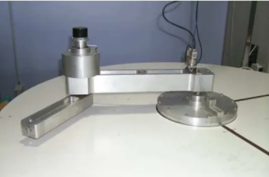
The identification method is carried out on a 2 degrees of freedom planar direct drive prototype robot without gravity effect, shown on Fig. 5. This direct drive prototype is very well suited to our purpose because it emphasizes non linear coupling when classical industrial robots with gear ratio above 50, divides this non-linear phenomenon by at least 2500. Moreover, the dynamic model of this robot includes eight parameters which allows us to present sev-eral conditions for the identification. At last, this robot and its real parameters, called the nominal parameters, are well known. Thus, we can check the physical meaning of the identified parameters.

The description of the geometry of the robot uses the modified Denavit and Hartenberg (DHM) notations (W.

Khalil et Kleinfinger 1986) which are illustrated on Fig. 6. The robot is direct driven by 2 DC permanent magnet mo-tors supplied by PWM amplifiers.

Fig. 5: The scara robot prototype.

x0 q₁ L O , O0 1 x1 x2 O2 y2 y0 y1 y2 q2

Fig. 6: DHM frames of the scara robot.

The dynamic model depends on 8 minimal dynamic pa-rameters, considering 4 friction parameters:

[

]

T 1R 1 1 2 R 2 2 2 2 ZZ Fv Fc ZZ LMX LMY Fv Fc χ= (52) 2 1R 1 1 2 ZZ =ZZ +Ia +M L 2 R 2 2 ZZ =ZZ +Ia

L =0.5m, is the length of the first link.

In the case of the SCARA robot, the parameters, LMX , ₂

and LMY , are identified instead of, ₂ MX , and ₂ MY , re-₂

spectively.

The 8 columns,IDM:,k, k=1,8, of IDM q,q,q

(

& &&

)

, in

0 0 0 1 R 1 1 2 R 2 1 1 :,1 ZZ :,2 Fv 1 2 1 :,3 Fc :,4 ZZ 1 2 ) 1 2 2 2 1 2 2 :,5 LMX 2 1 2 1 q q

IDM IDM , IDM IDM , q q sign( q )

IDM IDM , IDM IDM ,

q q ( 2q q ) cos q - q ( 2q q sin q IDM IDM q cos q q sin +     = =  = =      +     = =  = =  +     + = = + && & && && & && &&

&& && & & &

&& & 0 0 2 2 2 2 ) 1 2 2 2 1 2 2 :,6 LMY 2 1 2 1 2 :,7 Fv :,8 Fc 2 2 , q ( 2q q ) sin q q ( 2q q cos q IDM IDM , q cos q q sin q IDM IDM , IDM IDM

q sign( q ) +       − + −   = =  −       = =  = =     

&& && & & &

& &&

& &

(53) The closed-loop control is a PD control law (40) , ac-cording to Fig. 3, with:

2

1 1R 2 R 2

J =ZZ +ZZ + LMX , and J₂ =ZZ_{2 R}.

The actual gains are calculated with (45), taking a de-sired damping, dζ_j=1, for joint 1 and joint 2.

The desired natural frequency, dω_nj, is chosen according to the driving capacity without saturation of the joint drive. For this robot we obtain a full bandwidth with,

1 /

1

d f

n rd s

ω = , and dω =nf₂ 10rd s/ .

The sample rates of the control and of the measurement are equal to, f_m=200Hz.

Torque data are obtained from (41), and from the current reference data vτ.

The simulation of the robot is carried out with the same reference trajectory and with the same control law struc-ture as the actual robot.

The gains in the simulator are calculated with (46) and

with the same values,d

j ζ =1, 1 / 1 d n rd s ω = , and 10 / 2 d n rd s ω = .

The new identification process is performed in different cases in order to compare the previous IDIM technique to the new IV technique and to investigate the robustness of IV with respect to the initialization, to the data filtering and to the closed-loop tuning. All the results are given in SI units, on the joint side.

4.2. Comparison of IDIM and IV with good initial

values, χ_ˆ0=χ_ˆIV_.

At first, the algorithm is initialized with, χˆIDIM , the vector of parameters identified with the IDIM LS estimator.

The IDIM LS off-line estimation is carried out with a filtered position ˆq, calculated with a 20Hz cut-off fre-quency forward and reverse Butterworth filter, and with the velocities ˆq&, and the accelerations, &&ˆq, calculated with a central difference algorithm of ˆq. The parallel

decima-tion of Y_fm and W_fm, in (10), is carried out with a sample rate divided by a factor, n_d =20, and a lowpass filter cut-off frequency equal to, 0.8*fm/(2*nd)=4Hz.The results of

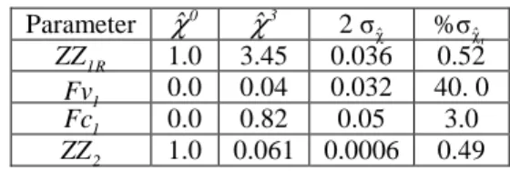
the IDIM identification are given in Table 1.

Starting with good initial values χˆ0=χˆIV, IV algo-rithms converges in only 2 steps to obtain the optimal solu-tion as shown in the table 2. The IV solusolu-tion is very close to the IDIM solution. Hence, the IV method does not im-prove the IDIM solution calculated with good bandpass filtered data.

A validation is plotted on Fig 7, at the frequency meas-urement, f_m=200Hz. It shows that the actual joint torques,

( )

fm

Y τ , and the torques estimated with the identified

mod-el,

(

2

)

, 2

e fm ddm ddm ddm ˆ ˆ

Y =W_δ q ,q& ,q&& χ χ are very close.

Both methods give a small relative norm error,

ˆ

Y−Wχ / Y <3%, which shows a good accuracy for the

model and for the identified values.

It can be seen that the parameters, Fv₁, and Fv₂, have no significant estimations because of their large relative standard deviation (>30%). They have no significant con-tribution in the joint torques and they can be cancelled to keep a set of essential parameters of a simplified dynamic model, without loss of accuracy (W. Khalil, Gautier, et Lemoine 2007).

However, we prefer to keep all the parameters in the following, for a better comparison of IDIM and IV identi-fication methods. 4000 4500 5000 5500 6000 -15 -10 -5 0 5 10 15 Joint 1 M o to r to rq u e ( N m ) Sample number Measurement: Yfm Estimation: Ye Error = Yfm - Ye -1 -0.5 0 0.5 1 Joint 2 M o to r to rq u e ( N m ) Measurement: Yfm Estimation: Ye Error = Yfm - Ye

Fig. 7.IV validation

Table 1: IDIM identification Parameter χ_ˆIDIM χ 2 σˆ %σˆχr 1R ZZ 3.44 0.034 0.50 1 Fv 0.03 0.031 52. 0 1 Fc 0.82 0.1 6.0 2 ZZ 0.062 0.0006 0.51 2 LMX 0.121 0.0014 0.56 2 LMY 0.007 0.0007 5.0 2 Fv 0.013 0.006 23.0 2 Fc 0.137 0.006 2.30 IDIM ˆ Y−Wχ / Y =0.024 Table 2: IV identification Parameter χˆ2 2 σˆ_χ %σχˆr 1R ZZ 3.44 3.45 0.036 0.52 1 Fv 0.03 0.04 0.032 40. 0 1 Fc 0.82 0.82 0.05 3.0 2 ZZ 0.062 0.061 0.0006 0.49 2 LMX 0.121 0.124 0.0013 0.52 2 LMY 0.007 0.007 0.0005 3.5 2 Fv 0.013 0.013 0.0084 30.0 2 Fc 0.137 0.137 0.008 3.0 IV ˆ Y−Wχ / Y =0.021

4.3. IV, validation of the regular initialization,

0 2

( ddm,ˆ )=

M q χ I .

The robustness of IV with respect to a wrong initializa-tion, such as the regular initialization (50), is investigated.

The initial values of the dynamic parameters are given by (48), with:

[

]

T 1 0 0 1 0 0 0 0 0 ˆ χ =

The identified values given in Table 3, are very close to those given in Table 1. This result validates the regular ini-tialization procedure.

Moreover the algorithm converges in only 3 steps and is not time consuming.

Table 3: IV identification with regular initialization

Parameter χ_ˆ0 χ_ˆ3 χ 2 σˆ %σˆχr 1R ZZ 1.0 3.45 0.036 0.52 1 Fv 0.0 0.04 0.032 40. 0 1 Fc 0.0 0.82 0.05 3.0 2 ZZ 1.0 0.061 0.0006 0.49 2 LMX 0.0 0.124 0.0013 0.52 2 LMY 0.0 0.007 0.0005 3.5 2 Fv 0.0 0.013 0.0084 30.0 2 Fc 0.0 0.137 0.008 3.0

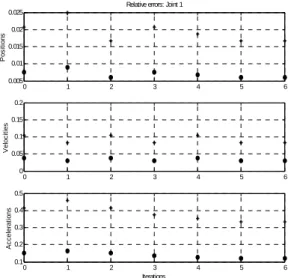
The relative norm errors on joint position, velocity and acceleration are plotted on Fig.8 ,with the following leg-end:

• norm error relative to the actual filtered joint position, j ddm ˆj ˆj q −q / q , velocity j ddm ˆj ˆj q −q / q

& & & , and

accel-eration, j

ddm ˆj ˆj q −q / q

&& && && , where

( )

ˆq,q,q& &&ˆ ˆ , are calculated

as given in section 4.2.

* norm error relative to the reference joint position,

j j j ddm r r q −q / q , velocity, j j j ddm r r q −q / q

& & & , and

accel-eration,

j j j

ddm r r q −q / q

&& && && .

The assumption (35),

(

qddm(ˆχk),q&ddm(ˆχk),q&&ddm(ˆχk)

)

( )

q,q,qˆ & &&ˆ ˆ , at each iteration

k, is confirmed Fig. 8, with a constant relative norm error close to 0.5% for the position, 5%, for the velocity and 10%, for the acceleration.

These results validate the updating procedure (46), of the simulated PD control law gains.

It can be seen also on Fig 8 that the simulated trajectory,

(

qddm(χˆk),q&ddm(ˆχk),q&&ddm(ˆχk)

)

, is 3 to 5 times closer to

the actual one,

( )

ˆq,q,q& &&ˆ ˆ , than to the reference one,

(

q ,q ,qr & &&r r

)

, with a relative norm error close to 1.5% for the position, 15%, for the velocity and 30%, for the accel-eration. Moreover, this error depends on the closed-loop bandwidth. It means that computing the observation matrix in (13) with the reference trajectory,

(

q ,q ,q_r & &&_{r r}

)

, leads to a bad identification of the dynamic parameters.

Then, the assumption

0 0.5 1 1.5 2 2.5 3 0 0.005 0.01 0.015 0.02

Relative errors: Joint 1

P o s it io n s 0 0.5 1 1.5 2 2.5 3 0.02 0.04 0.06 0.08 V e lo c it ie s 0 0.5 1 1.5 2 2.5 3 0.05 0.1 0.15 0.2 0.25 A c c e le ra ti o n s Iterations 0 0.5 1 1.5 2 2.5 3 0 0.005 0.01 0.015 0.02

Relative errors: Joint 2

P o s it io n s 0 0.5 1 1.5 2 2.5 3 0 0.05 0.1 0.15 0.2 V e lo c it ie s 0 0.5 1 1.5 2 2.5 3 0 0.1 0.2 0.3 0.4 A c c e le ra ti o n s Iterations

Fig. 8: • norm error relative to the filtered actual position, veloc-ity, acceleration. * norm error relative to the reference position,

velocity, acceleration. 0 0.5 1 1.5 2 2.5 3 0 0.005 0.01 0.015 0.02

Relative errors: Joint 2

P o s it io n s 0 0.5 1 1.5 2 2.5 3 0 0.05 0.1 0.15 0.2 V e lo c it ie s 0 0.5 1 1.5 2 2.5 3 0 0.1 0.2 0.3 0.4 A c c e le ra ti o n s Iterations

Fig. 9: • norm error relative to the filtered actual position, veloc-ity, acceleration. * norm error relative to the reference position,

velocity, acceleration.

The fast convergence of each parameter is shown in Table 4 , and is plotted on Fig 10.

Table 4: Parameters convergence with IV identification

Parameter χ_ˆ0 χ_ˆ1 χ_ˆ2 χ_ˆ3 1R ZZ 1.0 3.46 3.45 3.45 1 Fv 0.0 0.04 0.02 0.02 1 Fc 0.0 0.82 0.85 0.85 2 ZZ 1.0 0.06 0.061 0.061 2 LMX 0.0 0.122 0.124 0.124 2 LMY 0.0 0.05 0.07 0.07 2 Fv 0.0 0.005 0.01 0.01 2 Fc 0.0 0.130 0.132 0.132 0 1 2 3 1 2 3 4 Z Z 1 R 0 1 2 3 0 0.02 0.04 F V 1 0 1 2 3 0 0.5 1 F C 1 0 1 2 3 0 0.5 1 Z Z 2 0 1 2 3 0 0.1 0.2 M X 2 0 1 2 3 0 0.05 0.1 M Y 2 0 1 2 3 0 0.005 0.01 F V 2 Iterations 0 1 2 3 0 0.1 0.2 F C 2 Iterations

Fig. 10: IV parameters convergence

0 0.5 1 1.5 2 2.5 3 0 0.1 0.2 0.3 0.4

Relative error: Joint torque 1

Iterations 0 0.5 1 1.5 2 2.5 3 0 0.5 1 1.5 2 2.5 3

Relative error: Joint torque 2

Iterations

Fig. 11. IV, convergence of the joint torque error,

j j

_ˆ

k j

Y

−

W

χ

/ Y

We have seen that

k, with a constant small error. On the contrary, the relative torque norm error, given in Table 3, and plotted on Fig 12, dramatically decreases in only 3 steps. This shows the fast algorithm convergence.

4.4. Comparison of IDIM and IV, without data

filtering.

All the actual and simulated data are sampled at f_m= 200Hz.

The IDIM LS estimation is carried out with the measured joint position q, and with

( )

& &&ˆ ˆq,q , calculated by a central difference algorithm of q, without lowpass Butterworth filtering. There is no parallel decimation. IDIM Results are given in Table 5

IV starts with the regular initialization. IV Results are giv-en in Table 6.

Table 5: IDIM identification results without data filtering Parameter χˆIDIM 2 σ_χˆ %σχˆr 1R ZZ 1.5 0.05 1.6 1 Fv 0.095 0.15 80.0 1 Fc 0.55 0.26 23.3 2 ZZ 0.14 0.018 6.7 2 LMX 0.63 0.035 2.7 2 LMY 0.1 0.023 11.8 2 Fv 0.001 0.143 700.0 2 Fc 0.19 0.244 68.40 IDIM ˆ Y−Wχ / Y =0.8

Table 6: IV identification results without data filtering

Parameter χˆ0 χ_ˆ2 χ 2 σˆ %σˆχr 1R ZZ 1.0 3.45 0.007 0.1 1 Fv 0.0 0.05 0.023 21.0 1 Fc 0.0 0.81 0.004 0.24 2 ZZ 1.0 0.061 0.0004 0.3 2 LMX 0.0 0.124 0.0015 0.3 2 LMY 0.0 0.008 0.0009 5.6 2 Fv 0.0 0.023 0.0022 48.0 2 Fc 0.0 0.13 0.0038 1.5 IDIM ˆ Y−Wχ / Y =0.08

The identified values with IDIM are not good while the identified values with IV are still good.

IDIM fails because of the too large noise in the observa-tion matrix, W_fm

( )

q,q,q& &&ˆ ˆ , coming from the derivation of

q, without lowpass filtering. Then the LS estimation is biased.

IV succeeds because the observation matrix,

(

, k

)

fm ddm ddm ddm ˆ

W_δ q ,q& ,q&& χ , is calculated without noise with

the simulated values

(

q_ddm,q&_ddm,q&&_ddm

)

.

This validation shows that IV cancels the bias of IDIM es-timation, coming from a noisy estimation of

( )

ˆq,q,q& &&ˆ ˆ , which gives a too noisy observation matrix W_fm

( )

q,q,q& &&ˆ ˆ .

4.5. IV robustness with respect to error in the

si-mulated closed-loop tuning, dω_n

This section investigates the effect of an error between the actual value, a

n

ω , and the simulated value d

n

ω , of the natural frequency which represents the closed-loop band-width.

The IV identification is performed taking half the values

of the full ones given in section 3.4,

/2=1/2 (rd/s)

1 1

d d f

n n

ω = ω and dωn₂ = dωnf₂ / 2=10/2 (rd/s),

and the same procedure used to obtain results shown in Table 2, that is to say a frequency measurement,

m

f =200Hz, and a parallel decimation with a factor,

d

n =20, and a lowpass filter cut-off frequency equal to

4Hz.

The parameters, given in Table 7, converge in only 6 steps to values which are very close to those obtained in Table 2,

with a full closed-loop bandwidth.

Table 7: IV with half full bandwidth

Parameter χ_ˆ0 χ_ˆ6 χ 2 σˆ %σχˆr 1R ZZ 1.0 3.44 0.014 0.2 1 Fv 0.0 0.02 0.012 15.0 1 Fc 0.0 0.86 0.016 1.0 2 ZZ 1.0 0.060 0.0001 0.1 2 LMX 0.0 0.124 0.0002 0.1 2 LMY 0.0 0.007 0.0003 2.0 2 Fv 0.0 0.01 0.003 10.0 2 Fc 0.0 0.13 0.0008 0.3

The relative norm errors on joint position, velocity and acceleration are plotted on Fig 11, with the same legend as previously.

It can be seen that,

(

qddm(ˆχk),q&ddm(ˆχk),q&&ddm(ˆχk)

)

( )

q,q,qˆ & &&ˆ ˆ , at each iteration

k, with a constant norm error larger but close to the value obtained with the full bandwidth, Fig.11, close to, 0.5% for the position, 5%, for the velocity and 10%, for the accel-eration.

0 1 2 3 4 5 6 0.005 0.01 0.015 0.02 0.025

Relative errors: Joint 1

P o s it io n s 0 1 2 3 4 5 6 0 0.05 0.1 0.15 0.2 V e lo c it ie s 0 1 2 3 4 5 6 0.1 0.2 0.3 0.4 0.5 A c c e le ra ti o n s Iterations

Fig. 12: • norm error relative to the filtered actual position, veloc-ity, acceleration. * norm error relative to the reference position,

velocity, acceleration. 0 1 2 3 4 5 6 0 0.01 0.02 0.03

Relative errors: Joint 2

P o s it io n s 0 1 2 3 4 5 6 0 0.05 0.1 0.15 0.2 V e lo c it ie s 0 1 2 3 4 5 6 0.1 0.2 0.3 0.4 0.5 A c c e le ra ti o n s Iterations

Fig. 13: • norm error relative to the filtered actual position, veloc-ity, acceleration. * norm error relative to the reference position,

velocity, acceleration.

The relative torque norm error, given in Table 9, and plotted on Fig 12, decreases in 6 steps, only twice more than with the full bandwidth (see Table 3). This shows that IV is not very sensitive to error in the simulated closed-loop bandwidth, provided the control law structure is known.

However, IV fails beyond 1/3 of the full bandwidth, with

3

d d f n n /

ω ≤ ω .

5. Discussion and conclusion

One of the improvements of our algorithm is to avoid the acceleration calculation. It is one of the major difficult

points of the LS identification technique. In the general case, this problem is solved by a suitable data filtering. But, the choice of the cut-off frequency is crucial. If the cut-off frequency is too low the system is ill-conditioned and the main parameters are badly identified. On the other hand, if the cut-off frequency is too large, the observation matrix is strongly noisy and the LS estimator is biased. It is the reason why some techniques have been developed to overcome this problem: by integrating the dynamic model (Slotine et Weiping Li 1987)(Middleton et Goodwin 1988) or by using the power (Gautier 1997). The drawback of the method integrating the dynamic model is the complex ex-pression of the model. The drawback of the power model is the loss of information due to the mix of torques. Indeed, the dynamic effect of the wrist is negligible compared to the effect of the first three axes.

The IV method is not affected by these problems be-cause we keep all dynamic equations. In addition, the IV is less sensitive to the choice of cut-off frequency compared with the LS technique. From our point of view, our algo-rithm acts implicitly as an adaptative filter. Indeed, the high frequency noises are eliminated thanks to the integra-tion of the MDD while the frequency bandwidth of our in-terest is determined by the bandwidth of the closed loop. Finally, experimental results have proven that the prefilter-ing is not necessary.

Another major improvement of our approach is to en-sure the bandwidth of the closed loop in the simulator scheme. By this way, we have always q ,q ,q_S & &&_{S S}close to

q,q ,q& && . The correlation between the instrument matrix and the observation matrix is still high because V is still

close to Wnf. That means we ensure the crucial assumptions

T

E(V ρ )=0 and V WT invertible, and this explains why our algorithm works very well.

Our approach can be seen as an extension of the so-called SRIVC algorithm (Simplified Refined Instrumental Variable Continuous-time) adapted recently for closed loop system (Gilson et al. 2006) (Young, Garnier, et Gil-son 2009). However, these algorithms are quite compli-cated and need prefiltering. They do not adapt the gain of the simulated feedback as it is proposed in this paper. Therefore, our method is not only an application of the IV to robotics but enrich the IV methodology by providing insights from robotics.

With our algorithm, the inverse and direct dynamic models are both validated at the same time. Up to now, the DDM was validated a posteriori in simulation. This is in-teresting for industrial applications because this algorithm saves time. In addition, if something goes wrong, that means the dynamic model is not valid since the IV method is robust to data filtering.

This paper has presented an extension and an application of the IV method. This technique was successfully applied on a 2 DOF prototype robot. From these experiments, it comes that our IV algorithm is not sensitive to data