HAL Id: hal-00280278
https://hal.archives-ouvertes.fr/hal-00280278
Submitted on 30 Mar 2020
HAL is a multi-disciplinary open access
archive for the deposit and dissemination of
sci-entific research documents, whether they are
pub-lished or not. The documents may come from
teaching and research institutions in France or
abroad, or from public or private research centers.
L’archive ouverte pluridisciplinaire HAL, est
destinée au dépôt et à la diffusion de documents
scientifiques de niveau recherche, publiés ou non,
émanant des établissements d’enseignement et de
recherche français ou étrangers, des laboratoires
publics ou privés.
Distributed under a Creative Commons Attribution| 4.0 International License
Synergy of active and passive satellite microwave data
for the study of first-year sea ice in the Caspian and
Aral seas
A.V. Kouraev, F. Papa, N.M. Mognard, P.I. Buharizin, A. Cazenave, J.-F.
Crétaux, J. Dozortseva, F. Remy
To cite this version:
A.V. Kouraev, F. Papa, N.M. Mognard, P.I. Buharizin, A. Cazenave, et al.. Synergy of active and
passive satellite microwave data for the study of first-year sea ice in the Caspian and Aral seas. IEEE
Transactions on Geoscience and Remote Sensing, Institute of Electrical and Electronics Engineers,
2004, 42 (10), pp.2170-2176. �10.1109/TGRS.2004.835307�. �hal-00280278�
Synergy of Active and Passive Satellite Microwave
Data for the Study of First-Year Sea Ice
in the Caspian and Aral Seas
Alexei V. Kouraev, Fabrice Papa, Nelly M. Mognard, Petr I. Buharizin, Anny Cazenave, Jean-Francois Cretaux,
Julia Dozortseva, and Frederique Remy
Abstract—The paper discusses application of active and passive
microwave data for assessment of time and space variations of first-year ice cover. The Caspian and Aral Seas are chosen as main study areas. The Caspian Sea evolution is primarily climate driven, while for the Aral Sea there is a mix of anthropic and climate factors. We analyze ice cover conditions using a novel method that combines active and passive satellite measurements for ice discrimination. This method uses the synergy of simultaneous data from active (radar altimeter) and passive (radiometer) microwave instruments onboard the TOPEX/Poseidon (T/P) satellite, launched in 1992. The benefits, drawbacks, and potential of ice cover studies using the proposed method are discussed. We analyze in detail how this method is influenced by the difference in footprints of the T/P sen-sors and by the radiometric properties of ice and snow at different stages of ice cover evolution. In order to link the T/P-derived re-sults to historical observations that end in the mid-1980s, long time series of passive microwave data from SMMR and SSM/I sensors have also been analyzed. Satellite time series of ice cover extent and duration of ice period have been obtained for the Caspian and Aral Seas since 1978. A good agreement is obtained between historical and satellite data, with significant spatial and temporal variability of ice conditions. There is a marked decrease of both duration of ice season and ice extent during the winters 1998/1999–2001/2002. These satellite-derived time series of sea ice parameters are very valuable in view of the heterogeneous and mostly unpublished data on ice conditions over the Caspian and Aral Sea since the mid-1980s.
Index Terms—Aral Sea, Caspian Sea, combination of active and
passive microwave data, first-year sea ice, radar altimetry.
I. INTRODUCTION
T
HE PRESENCE of ice cover influences human activities in many parts of the world. Studies and monitoring of ice conditions is thus important for maritime safety and sustainableA. V. Kouraev is with the Laboratoire d’Etudes en Géophysique et Océanographie Spatiales, Observatoire Midi-Pyrenees, Centre Na-tional d’Etudes Spatiales, 31401 Toulouse, France (e-mail: kouraev@ notos.cst.cnes.fr), on leave from the State Oceanography Institute, St. Peters-burg branch, St. PetersPeters-burg, Russia.
F. Papa, N. M. Mognard, A. Cazenave, J-F. Cretaux, and F. Remy are with the Laboratoire d’Etudes en Géophysique et Océanographie Spatiales, Observatoire Midi-Pyrenees, Centre National d’Etudes Spatiales, 31401 Toulouse, France.
P. I. Buharizin is with the Water Problems Institute, Russian Academy of Sciences, Astrakhan Division, Astrakhan, Russia.
J. Dozortseva is with the Hydrometeorological Centre of the Caspian Fleet, Astrakhan, Russia.
environmental management. Nowadays, a significant part of sea ice routine monitoring is done by satellite microwave observa-tions, which provide reliable, consistent, weather-independent, and easily accessible data on ice cover.
For more than two decades, the scientific community has used passive microwave data from the Scanning Multichannel Microwave Radiometer (SMMR) and the Special Sensor Mi-crowave/Imager (SSM/I) instruments to estimate ice cover extent and type both in the Arctic and in the Antarctic. This technique requires a good knowledge of the radiometric properties of the ice for each specific region. However, in the case of the Caspian and Aral Seas, there are no available in situ measurements of ice cover and its properties to validate the ice discrimination algorithms. The Caspian and Aral Seas have been influenced by dramatic sea level changes during the last century [1]–[3]. Between the early 1920s and the late 1970s, the level of the Caspian Sea has fallen, and in 1977, the level has decreased by 3 m and reached its lowest mark for the last 400 years ( m below the sea level). Since then, the sea level began to rise to m in 1987, m in 1992, and in 1995. After 1995, the level started to slowly decrease again. The Caspian Sea level changes are explained by natural variability of the main constituents of the sea water budget, mostly by runoff from the Volga River [4]. No significant changes in the salinity of the sea (average salinity 7–9 ppt for the northern Caspian and 12–14 ppt for the middle Caspian) were observed.
The Aral Sea level was relatively stable until the early 1960s, when consumption of river water for agricultural purposes out-weighed the incoming part of the water budget. The equilibrium of the water budget was broken, and between 1960 and 1987, when the sea level dropped by 13 m, the sea surface decreased by 40%, and the averaged salinity increased from 10 to 28 g/l. In 1989, the level fell by another meter, and the sea was then divided into two separate basins: the Small Aral in the north and the Great Aral in the south, connected by a small channel where a dam was built later. The construction of the dam helped to stabilize the level and salinity of the Small Aral Sea [5], but the level of the Big Aral Sea continues to decrease and its salinity to increase. Ice cover forms every winter in the Caspian and the Aral Seas and stays for several months, negatively affecting the navigation conditions and the economic activity in the coastal areas and on the shelf, as for instance the Russian and Kazakh oil rigs operating in the northern Caspian.
The ice processes in the Caspian and Aral Seas have sig-nificant temporal and spatial variability, influenced by climate conditions, wind fields, and water currents, as well as sea mor-phology. Both seas are located on the far southern boundary of
sea ice cover development in the Northern Hemisphere. Due to this marginal location, data on ice variability in these seas may serve as an early indicator of regional climate change [6].
Regular studies of ice cover in the Caspian and Aral Seas started in the first half of the 20th century [1], [7] with in situ observations and aerial surveys, but existing published time se-ries of ice cover parameters stopped in 1984 to 1985. For the past two decades, the data are kept in local archives. Such in-formation is fragmentary, exists in heterogeneous form (data of aerial surveys, satellite imagery, data from ship observations, etc.), and is generally not available to the public [8].
Thus, satellite measurements provide means to continue times series of ice cover parameters necessary for practical applications, e.g., ship routing, protection of industrial objects, studies of environmental conditions and climate variability, and forcing and verification of general circulation models [9].
We present a synergy of simultaneous active and passive mi-crowave data from the TOPEX/Poseidon (T/P) satellite to un-ambiguously discriminate ice and open water in the absence of
in situ measurements and of radiometric properties of the ice.
We first describe the data and their selection, and explain the method to discriminate open water from ice. We then apply our method to derive a T/P time series of sea ice extent evolution. Then we complement them with observations from SMMR and SSM/I to obtain time series of ice extent and ice period duration for the Caspian and Aral Seas and compare the satellite-derived data with historical observations. The satellite time series of ice cover parameters show significant changes in the ice conditions in the last two decades. These results are probably the first at-tempt to fill in this important information gap in the ice cover information for the Caspian and Aral Seas since the mid-1980s.
II. DATA ANDDATASELECTION
A. Data Sources
The study of ice cover uses two data sources. The main one is observations from the TOPEX/Poseidon (T/P) satellite, operating since 1992. This platform has two nadir–looking instruments: 1) a dual–frequency radar altimeter (NASA radar altimeter—NRA) operating in C- and Ku-bands 5.3 and 13.6 GHz, respectively, and 2) a passive microwave radiometer (TMR) operating at 18, 23, and 37 GHz, (used to correct altimetric height measurements for atmospheric effects). The satellite has a repeat period of ten days and we use the 1-Hz data, which provide an along-track ground resolution of about 6 km. We have used the T/P data for cycles 1–360 (from the end of October 1992 to the end of June 2002).
In order to link T/P data with the available historical series, that end in mid 1980s, this information was complemented by the second source of data—more than 20-year-long passive mi-crowave observations from the scanning radiometers—SMMR (1979–1987) onboard NIMBUS-7 and SSM/I (since 1987) on-board the DMSP (Defence Meteorological Satellite Program) series. The National Snow and Ice Data Center (NSIDC) pro-vided the SMMR and SSMI data mapped to the Equal Area (625-km resolution) SSM/I Earth Grid (EASE-Grid) [10], [11]. The initial data were averaged in pentad (five days) mean values to obtain a continuous spatial coverage.
B. Data Selection
To account for the variability of the sea level and to ensure that observations do not cover land regions (that would
other-Fig. 1. T/P ground tracks over the northern Caspian (bold black line: data used) and EASE–grid pixels used for western and eastern parts (delimited by bold gray line). Depth labels (in meters) are also marked.
Fig. 2. T/P ground tracks over the Aral Sea (bold black line: data used) and EASE–grid pixels used (delimited by bold gray line). Changes in location of the coastline are shown for 1966 (black line), 1992 (dotted black line), and in 2002 (bold gray line).
wise contaminate the measurements) a geographical selection of the data was done (Figs. 1 and 2). T/P data closer than 20 km from the coast and SMMR and SSM/I EASE-grid pixels cov-ering coastal regions or islands were not used. For the Aral Sea, the data were selected using the location of coastline under the lowest sea level mark (in 2002).
III. ICEDISCRIMINATIONMETHODOLOGY
A. TOPEX/Poseidon Data—Synergy of Active and Passive Microwave Observations
1) Main Approach: Satellite altimetry for sea ice studies
started with the Seasat altimeter in 1978,and used the variability of the radar backscatter over the ice [12]. The backscatter is the ratio of the power reflected from the surface to the inci-dent power emitted by the radar altimeter, and is expressed in decibels. Recent studies use satellite altimeter measurements to estimate the ice freeboard and assess ice thickness in the Arctic [13]. These approaches only use data from the radar altimeter.
Fig. 3. Mean annual distribution of observations for T/P cycles 1–360 for the northern Caspian in the space of backscatter coefficient at 13.6 GHz versus the average value of brightness temperature at 18 and 37 GHz.
Though the primary instrument onboard T/P is the radar al-timeter and the primary mission is to measure sea level, we have found that the combination of simultaneous active and passive microwave measurements can be successfully used to study ice cover [8], [14], [15]. The method consists in analysing the T/P data in the space of two parameters. The backscatter coeffi-cient (called ) at 13.6 GHz is obtained from the NRA. The second parameter is the average value between the brightness temperature from TMR at 18 and 37 GHz [16] (we will call this TB/2), measured in Kelvin. The distribution of observations in this space yields two clusters, representing open water and ice (Fig. 3). Open water (observations in the lower left corner) has a low backscatter coefficient (10–12 dB) and low brightness tem-perature (TB/2 between 140–170 K). Sea ice (observations in the upper right corner) is characterized by a high backscatter coefficient (up to 40–42 dB) and high brightness temperatures (TB/2 between 220–260 K). For both sensors, the difference in the signal range between open water and ice is largely superior than the sensor noise estimated at 0.5 dB over continental re-gions [19].
Using only one of these parameters (backscatter coeffi-cient or TB/2) leads to ambiguities, e.g., when is between 20–30 dB or when TB/2 is between 180–220 K. However, their combination reveals the existence of two well-separated clusters and makes the discrimination between ice and open water more significant.
The ice observations form a distinctive cluster located in the upper right part of the distribution field (see Fig. 3). This cluster has a complicated shape, with many observations located in the lower corner of the ice cluster (high backscatter and low TB/2 values), as well as in the upper left corner (low backscatter and high TB/2). This behavior, (Sections II and III) is determined by several factors, such as the footprint size and the temporal variability of the dielectric properties of the ice cover.
2) Footprint Geometry: When looking at the distribution of
T/P observations in the space of backscatter (TB/2), the influ-ence of the footprint size is important. The average NRA foot-print diameter in Ku-band is between 10–12 km (depending on the surface roughness), while the TMR operating at 18, 23, and 37 GHz has a footprint diameter of 42, 35, and 22 km, respec-tively. By idealizing the TMR footprint as a circle, we may
rep-(a) (b)
Fig. 4. (a) Idealized representation of the T/P footprints for NRA in Ku-band and TMR at 37 and 18 GHz and (b) three types of ice edge used for simulation.
Fig. 5. Results of numerical simulations of variations of active and passive microwave signals when going from (A) open water to (D) a completely ice-covered region. The location of the observations for scenarios 1–3 is overlaid with isolines of number of observations for the northern Caspian (see Fig. 3).
resent them as three concentrical circles of various diameters (Fig. 4).
The signal from three sources comes simultaneously, but in the case of a heterogeneous surface, the difference in the spa-tial coverage will result in different values for the microwave parameters. Let us assume that open water and ice have typical backscatter and TB/2 values (Fig. 5, point A: open water; point D: ice). When a satellite flies from open water toward an ice-covered region and crosses the ice edge, its instruments would register changes in the backscatter and brightness temperatures. When all the three instruments have the same footprints, the signal follows the theoretical straight line between A and D. However, this is not the case for the T/P instruments. We have performed a numerical simulation to see how the signal would change for three different scenarios of ice edge shape (Fig. 4). In the first scenario, the ice edge is represented by a straight line, dividing 100% open water and 100% ice. In the second scenario, only half of all footprints will cover the ice-covered re-gion, which is a case similar to scenario 1 with 100% open water and 50% ice-covered concentrations. The third scenario repre-sent a relatively rare case when the ice field has the dimension comparable to theNRAfootprint (NRAwill only see ice, while TMR will see mostly open water and ice only in the central part of the footprint). The results of the simulations are plotted on Fig. 5 with constant time step.
For all three scenarios, the changes in the incoming signal start with changes in brightness temperature. The 18-GHz brightness temperature (TB) starts to increase first (slow in-crease of TB/2), followed by an inin-crease of the 37-GHz TB (leading to a more rapid increase of TB/2). The backscatter values do not change and T/P observations are distributed in the vertical direction between point A and B.
When the NRA footprint starts to cover the ice edge, both the backscatter and the TB/2 values rise. The measurements rapidly move from B to C, until the entire NRA footprint is over the ice. Then, the backscatter stays constant, while TB/2 continues to rise—first rapidly, then (when the entire 37-GHz TB footprint is over the ice)—more slowly. When all three instruments only see ice, point D is reached.
The results of the simulation for scenario 2 show a similar distribution, but the final point is E, which lies exactly halfway between A and D on the theoretical mixing line, representing 50% ice concentration. For scenario 3, the simulation ends at point F that has the same backscatter values as point D, but a TB/2 less than E (proportional to the percentage of ice and water coverage in the TB18 and TB37 footprints).
The distribution of the observations along these theoretical lines depends also very much on the ice conditions of each sea and on geometry of the T/P ground tracks relative to the ice edge location. For example, the simultaneous existence of several ice fields in the region covered by T/P ground tracks increases the probability of finding an ice edge in the T/P footprint and, thus, increases the total number of cases when the NRA senses only (or mostly) ice, while TMR senses mostly open water.
The observations located in the lower right portion of the ice cluster are associated with the different sizes of the NRA and TMR footprints. However, this does not explain existence of the observations in the upper left corner of the ice cluster, that have low backscatter and high TB/2 values. This issue is addressed in the following subsection.
3) Further Evolution of Ice: Once the ice starts growing, it
begins to get thicker and more rigid. Wind and currents forcing leads to ice deformation, to the formation of cracks and ridging, which increases the surface roughness. Snow accumulates, pref-erentially near the roughest surfaces.
At the end of the ice season this process is further compli-cated by melting/refreezing, appearance of pools of water on the ice, and by ice decay. All these processes change the dielectric properties of the ice and, thus, the microwave signal. In gen-eral, ice development, roughening and snow cover decrease the backscatter to 15–20 dB [16], while TB/2 stays relatively con-stant or even slightly increase (see Fig. 3).
Additional information on ice properties, especially when snow cover is present, may be inferred from the differences be-tween passive microwave measurements at different channels. Several snow cover algorithms have been developed for SMMR and SSM/I. To retrieve snow depth these algorithms use a linear relationship between the brightness temperature difference at 19 and 37 GHz and snow depth or snow water equivalent. Initially these algorithms were developed for application over land, but recently, using in situ data on snow depth in the Weddell, Bellinsgausen, and Amundsen Seas in the Antarctic, an algorithm for the SSM/I channels was developed [17] to retrieve snow depth over the sea ice
V V
V V (1)
Fig. 6. Mean values of snow depth in the northern Caspian derived from observations in the space of backscatter versus TB/2.
where is the snow depth, in centimeters, V and V are the brightness temperatures for ver-tical polarization at 37 and 19 GHz, respectively,
V V and V V ,
where open water brightness temperatures at the 19 and 37 GHz vertically polarized components are 176.6 and 200.5 K, and C—ice concentration. Assuming that the brightness temper-ature at 18 GHz does not differ significantly from the one at 19 GHz and taking into account that the T/P data are not polarized (consequently we are not able to estimate ice concen-tration, thus ), then the formula may be rewritten in the simplified form as
(2) Since this algorithm was developed for SSM/I that has an in-cidence angle of 53 , a correction should be taken when using data from the T/P nadir-looking radiometer [18]
(3) (with 53 the incidence angle for SSM/I)
Using (2) and (3) for the northern Caspian data, we found that the highest values of snow depth correspond to observa-tions located in the far left and lower part of the ice cover cluster (Fig. 6). Observations in these parts are usually obtained in mid-winter, what corresponds to the maximal snow development over the ice. Papa et al. [18] show that snow cover significantly decreases the backscatter values and that it rarely changes abso-lute values of the brightness temperature.
Thus, the observations in the upper left corner of the ice cluster are mostly associated with the development of snow cover on the ice. Though the lack of ground truth snow data for the northern Caspian or Aral Seas does not allow to fully quantify this relation or validate the snow depth estimates, the general temporal evolution of radiometric signals looks reasonable.
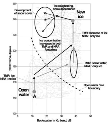
4) Resulting Schema of Ice Development: The specificity
of T/P microwave instruments, footprint geometry and various stages of ice cover development define typical succession of ob-servations in the space of backscatter versus TB/2. This develop-ment is schematically presented in Fig. 7 (for detailed sequence of mean monthly distribution of observations, see [14]).
Due to footprint geometry, ice is observed first by TMR (in-crease of TB/2), then by both NRA and TMR: backscatter and TB/2 increase until highest backscatter values (when NRA sees
Fig. 7. Schematic representation of the temporal evolution of T/P observations during winter in the space of backscatter versus TB/2. Schema is overlaid on isolines of number of observations for the northern Caspian (see Fig. 3).
only ice). When both sensors see only ice, observations are lo-cated in the center of the ice cluster, with values of backscatter and TB/2 typical of new ice. As the ice surface gets rough and when snow is present, the backscatter decreases, and TB/2 os-cillates slightly. Observations in the upper left part of the ice cluster may also represent cases when melt ponds start to ap-pear: NRA sees water when TMR senses predominantly ice.
We plan to perform more detailed comparison of T/P observations with in situ observations, historical ice charts, and other satellite data. After establishing statistically sound relations, estimations of ice concentration, ice roughness (and probably type), and snow depth could be made possible. For instance, we can take advantage of the dual-frequency NRA instruments to better constrain ice characteristics and evolution [19]. For the time being, we will apply our method only to discriminate between open water and ice, using a threshold line, shown in Fig. 7.
B. SMMR and SSM/I Algorithms
In order to fill the gap between the T/P-derived results that start in 1992 and historical observations, which end in mid-1980s, the time series of passive microwave data from SMMR and SSM/I sensors have been used. There are several approaches for estimating ice cover concentration using pas-sive microwave data [20]–[22]. Most of these algorithms use SMMR and SSM/I brightness temperature data from the 19.35 (18.0 for SMMR) and 37.0 GHz horizontally (H) and vertically (V) polarized channels.
Most of the ice algorithms (such as NASA Team or Bootstrap algorithms) were developed for Arctic or Antarctic conditions and need to be adapted and validated for the Caspian and Aral Seas. The absence of in situ measurements for the radiometric
properties of ice and snow in these seas is a problem for the se-lection of tie-points for these algorithms. Currently, we apply a simplified algorithm that uses the polarization (PR) and spectral (GR) gradient ratios with a threshold (defined as a linear rela-tionship between two sets of fixed PR and GR values for SMMR and SSM/I) in order to distinguish between ice and open water. No reliable estimation of ice concentration from SMMR and SSM/I data can be made at this stage. The combination of si-multaneous active and passive data from T/P presents the obser-vations as two distinctive clusters that allow to unambiguously discriminate between ice and open water. The observations from SMMR and SSM/I in the PR/GR space form two mixed clus-ters and ice discrimination is ambiguous. Therefore at this stage of development of ice discrimination methods for the Caspian and Aral Seas we consider T/P-derived ice cover parameters as having a higher data quality, while SMMR-SMM/I observations are less reliable and thus only complementary.
IV. RESULTS
Applying the methods described above to the T/P and SMMR-SSM/I data for the northern Caspian and Aral Seas, time series of beginning and end dates of ice season, of ice season duration and of ice cover extent were obtained. This satellite-derived dataset provides for the first time continuous time series of ice cover variability since the mid-1980s for the Caspian and Aral Seas.
A. Duration of the Ice Season
The formation of ice cover starts mostly in November-De-cember (and in the Aral Sea also in January), with the earliest dates October, 23–27. These dates agree well with the histor-ical observations [1], [7]. The end of the ice season usually occurs at the end of March or the beginning of April. In the Aral Sea, starting with the 1997/1998 winter, the end of the ice season shifted to January–February, and the ice season duration decreased from 80–120 to 10–40 days. In the eastern part of the northern Caspian Sea, the duration of the ice season appears stable, ranging from 90–140 days. However, in the western part a marked decrease in ice season duration is also observed: from 80–100 to 60–80 days.
Passive microwave radiometers are known to be poorly sen-sitive to new thin ice. At the same time the presence of an active microwave instrument onboard T/P allows to better identify new ice and small ice floes. As a result, the start and the end of the ice season are observed differently by T/P and SMMR-SSM/I (for more details see [8]). SMMR and SSM/I have a tendency to underestimate the duration of the ice season, while T/P pro-vides more precise observations.
B. Ice Extent
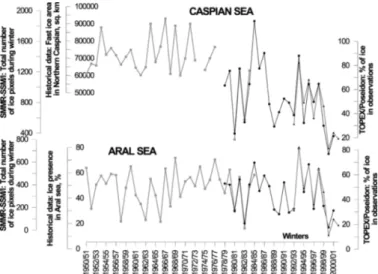
Satellite-derived series of ice extent were compared with available historical observations. These data series have dif-ferent scales and measurements units and sometimes refer to various regions. For the northern Caspian [7], the historical data available up to 1985 is the ice cover surface in square kilometers, with some gaps in the observations and an obvious change in the calculation method after 1977. For the Aral Sea, the historical data units are in percent of the sea surface [1]. For the SMMR and SSM/I data, in order to assess ice conditions for each winter, we computed the total number of ice pixels
Fig. 8. Ice cover extent in the Caspian and Aral Seas from historical (bold gray line with rectangles) and satellite observations: SMMR and SSM/I (black line with black circles) and T/P data (bold gray line with black triangles).
observed during October-April. Due to the limited spatial coverage of the TOPEX/Poseidon ground tracks, the variations of ice extent were assessed by computing for each overflight the ratio (in percent) of: 1) cases when observations were considered to have ice cover to 2) the total number of available 1-Hz observations for each ground track. These time series cannot be compared directly, but their superposition shows that at the winter time scale they all agree very well (Fig. 8).
Both seas are characterized by a “saw-like” variability of ice conditions, when milder and severe winter conditions alternate with 2–3 years interval. This variability is often superimposed on warming or cooling trends of larger scale. However, the con-tinuous decrease of ice extent observed since winter 1993/94, reaching in 1999/00 the lowest value for the whole period of observations, is evident.
For the Aral Sea, this may be partly explained by the contin-uing decrease of sea volume (and thus of heat storage capacity) and the increase of salinity that would have shifted the freezing temperature [8]. However, the observed changes in dates of the beginning and the end of the ice season and the decrease of ice extent is also evident in the Caspian Sea, where no significant changes in heat storage capacity or water salinity were observed. This indicates that both these seas respond similarly to regional climatic factors.
The observed warming signal poses the question: is it a long-term trend or just a series of mild winters? To answer this ques-tion, we need to analyze variability of ice cover as function of climatic parameters and to extend the time series with new data.
V. DISCUSSION
The combination of simultaneous data from nadir-looking ac-tive and passive sensors onboard the TOPEX/Poseidon satellite and passive microwave observations from SMMR and SSM/I looks very promising for studies of sea ice cover and, for the first time, provide continuous series of ice cover parameters for the Caspian and Aral Seas since mid-1980s.
The proposed methodology increases the capacity for dis-criminating open water and ice using the synergy of active and passive microwave observations. The T/P data that has a high radiometric sensitivity and an increased spatial resolution along
the satellite ground track offer a better capacity to detect the dates of the onset of ice formation and break-up, as well as ice edge detection (in the region covered by T/P ground tracks). Complementing these data with SMMR and SSM/I observa-tions, with wide spatial coverage and high temporal resolution increases our understanding of ice formation, development and decay.
Further validation and improvement of discrimination algo-rithms using in situ and satellite data will provide additional in-formation on ice concentration, ice roughness, and snow depth on ice. Additional improvement could be done by using data from similar sensors onboard other satellites, such as Jason-1 and Envisat. Jason-1 is now exactly following the initial T/P ground tracks, while since August 2002 T/P was put onto a new orbit, flying halfway between its previous tracks. This change of T/P orbit doubles the spatial coverage for the two satellites. While T/P and Jason-1 data are limited to a coverage between 66 N and 66 S, the European altimeter onboard Envisat over-flies larger areas (from 82 N to 82 S) and could be used as soon as the data become readily available. Moreover, its dual-fre-quency capability will help for the discrimination of sea ice characteristics.
We are currently analysing T/P and SMMR-SSM/I data for the Bothnian Bay in the Baltic Sea and the Hudson Bay in the Canadian Arctic, where T/P ground track coverage is much denser due to its orbital parameters. Higher spatial coverage and availability of in situ observations on ice type, extent, and roughness for these bays will permit to further develop and val-idate our approaches for synergistic use of active and passive microwave data.
The issue of recent warming is still open, but some con-sequences of changes in ice conditions are already visible. In the Caspian Sea, dramatic reduction of ice extent since 1998/1999 has affected breeding habits and living conditions for the Caspian seal, the only mammal in this sea. In winter, seals gather on the sea ice in the northern Caspian Sea, when they pup, nurse, mate and molt. The lack of stable ice cover leads to poor conditions for seal breeding. As a result, there is a weakening of their immune system aggravated by the spreading of viruses which may lead to cases of mass mortality, as it was observed in 2000 when between 20 000 and 30 000 seals were found dead [8].
REFERENCES
[1] V. N. Bortnik and S. P. Chistyayeva, Eds., Gidrometeorologiya
i Gidrohimiya Morey (Hydrometeorology and Hydrochemistry of Seas). Leningrad, Russia: Gidrometeoizdat, 1990, vol. VII, Aral Sea. [2] A. Cazenave, P. Bonnefond, K. Dominh, and P. Schaeffer, “Caspian sea level from Topex-Poseidon altimetry: Level now falling,” Geophys. Res.
Lett., vol. 24, no. 8, 1997.
[3] A. N. Kosarev and E. A. Yablonskaya, The Caspian Sea. The Hague, The Netherlands: SPB Academi, 1994.
[4] A. N. Kosarev and A. V. Kouraev, “About influence of the river Volga runoff on hydrological conditions of the Northern Caspy during modern sea level rise,” in International Hydrological Programme, IHP-V,
Tech-nical Documents in Hydrology, N3, Environmental and Socio-Economic Consequences of Water Resources Development and Management Proce. Moscow Symp., G. V. Voropaev and N. A. Zaitseva, Eds., Paris,
France, May 15–20, 1995, pp. 134–137.
[5] N. Aladin, J.-F. Crétaux, I. S. Plotnikov, A. V. Kouraev, A. O. Smurov, A. Cazenave, A. N. Egorov, and F. Papa, “Modern hydro-biological state of the Small Aral Sea,” Environmetrics, 2004, submitted for publication. [6] I. Allison, R. G. Barry, and B. Goodison, Eds., “Climate and Cryosphere (CliC) Project. Science and co-ordination plan. Version 1,” World Climate Research Programme, Geneva, Switzerland, WCRP-114 WMO/TD 1053, 2001.
[7] F. S. Terziev, A. N. Kosarev, and A. A. Kerimov, Eds.,
Gidrometeo-rologiya i Gidrohimiya Morey (Hydrometeorology and Hydrochemistry of Seas). St.-Petersburg, Russia: Gidrometeoizdat, 1992, vol. VI, Caspian sea, Issue 1—Hydrometeorological Conditions.
[8] A. V. Kouraev, F. Papa, N. M. Mognard, P. I. Buharizin, A. Cazenave, J.-F. Crétaux, J. Dozortseva, and F. Remy, “Sea ice cover in the Caspian and Aral seas from historical and satellite data,” J. Marine Syst., vol. 47, pp. 89–100, 2004.
[9] N. A. Rayner, R. W. Reynolds, and V. Smolyanitsky, “Climate research requirements for historical sea ice data,” in Abstracts of Workshop on
Sea-Ice Extent and the Global Climate System (15-17 April 2002) and Mini-Conference on Long-Term Variability of the Barents Sea Region (18-19 April 2002), Toulouse, France, 2002.
[10] P. Gloersen and E. Francis. (1997) NIMBUS-7 SMMR antenna temper-atures. Nat. Snow Ice Data Center, Boulder, CO
[11] R. L. Armstrong, K. W. Knowles, M. J. Brodzik, and M. A. Hardman, “DMSP SSM/I Pathfinder daily EASE-grid brightness temperatures,” Nat. Snow Ice Data Center, Boulder, CO, 1994.
[12] F. M. Fetterer, M. R. Drinkwater, K. C. Jezek, S. W. C. Laxon, R. G. On-stott, and L. M. H. Ulander, “Sea ice altimetry,” in Microwave Remote
Sensing of Sea Ice, Geophysical Monograph, F. D. Carsey, Ed. Wash-ington, DC: AGU, 1992, vol. 68.
[13] S. Laxon, N. Peacock, and D. Smith, “High interannual variability of sea ice thickness in the Arctic region,” Nature, vol. 425, no. 6961, pp. 947–950.
[14] A. V. Kouraev, F. Papa, P. I Buharizin, A. Cazenave, J.-F. Crétaux, J. Dozortseva, and F. Remy, “Ice cover variability in the Caspian and Aral seas from active and passive satellite microwave data,” Polar Res., vol. 22, no. 1, pp. 43–50, 2003.
[15] A. V. Kouraev, F. Papa, N. M. Mognard, P. I. Buharizin, A. Cazenave, J-F Crétaux, J. Dozortseva, and F. Remy, “Variations of sea ice extent in the Caspian and Aral seas derived from combination of active and passive satellite microwave data,” in Proc. IGARSS, vol. 4, 2003, pp. 2808–2810. [16] F. T. Ulaby, R. K. Moore, and A. K. Fung, Microwave Remote Sensing,
Active and Passive. Norwood, MA: Artech House, 1986, vol. III, From Theory to Applications.
[17] T. Marcus and D. J. Cavalieri, “Snow depth distribution over sea ice in the Southern Ocean from satellite passive microwave data,” in Antarctic
Sea Ice: Physical Processes, Interactions and Variability, M. O. Jeffries,
Ed. Washington, DC: AGU, 1998, vol. 74, Antarctic Research Series, pp. 19–39.
[18] F. Papa, B. Legresy, N. Mognard, E. G. Josberger, and F. Remy, “Estimating terrestrial snow depth with the TOPEX/Poseidon altimeter and radiometer,” IEEE Trans. Geosci. Remote Sensing, vol. 40, pp. 2162–2169, Oct. 2002.
[19] F. Papa, B. Legresy, and F. Remy, “Use of the TOPEX/Poseidon dual-frequency radar altimeter over land surfaces,” Remote Sens. Environ., 2004, to be published.
[20] K. Steffen, J. Key, D. J. Cavalieri, J. Comiso, P. Gloersen, K. S. Germain, and I. Rubinstein, “The estimation of geophysical parameters using pas-sive microwave algorithms,” in Microwave Remote Sensing of Sea Ice,
Geophysical Monograph, F. D. Carsey, Ed. Washington, DC: AGU, 1992, vol. 68.
[21] J. C. Comiso, “Characteristics of Arctic winter sea ice from satellite multispectral microwave observations,” J. Geophys. Res., vol. 91, pp. 975–994, 1986.
[22] C. T. Swift and D. J. Cavalieri, “Passive microwave remote sensing for sea ice research,” EOS, vol. 66, no. 49, pp. 1210–1212, 1985.