EEG BIOMETRICS DURING SLEEP AND WAKEFULNESS: PERFORMANCE OPTIMIZATION AND SECURITY IMPLICATIONS
ROCIO BEATRIZ AYALA MEZA
DÉPARTEMENT DE GÉNIE INFORMATIQUE ET GÉNIE LOGICIEL ÉCOLE POLYTECHNIQUE DE MONTRÉAL
MÉMOIRE PRÉSENTÉ EN VUE DE L’OBTENTION DU DIPLÔME DE MAÎTRISE ÈS SCIENCES APPLIQUÉES
(GÉNIE INFORMATIQUE) NOVEMBRE 2017
UNIVERSITÉ DE MONTRÉAL
ÉCOLE POLYTECHNIQUE DE MONTRÉAL
Ce mémoire intitulé :
EEG BIOMETRICS DURING SLEEP AND WAKEFULNESS: PERFORMANCE
OPTIMIZATION AND SECURITY IMPLICATIONS
présenté par : AYALA MEZA Rocio Beatriz
en vue de l’obtention du diplôme de : Maîtrise ès sciences appliquées a été dûment accepté par le jury d’examen constitué de :
M. PAL Christopher J., Ph. D., président
M. FERNANDEZ José M., Ph. D., membre et directeur de recherche M. JERBI Karim, Ph. D., membre et codirecteur de recherche
DEDICATION
Far better it is to dare mighty things, to win glorious triumphs, even though checkered by failure, than to rank with those poor spirits who neither enjoy much nor suffer much, because they live in that grey twilight that knows neither victory nor defeat.
RÉSUMÉ
L’internet des objets et les mégadonnées ont un grand choix de domaines d’application. Dans les soins de santé ils ont le potentiel de déclencher les diagnostics à distance et le suivi en temps réel. Les capteurs pour la santé et la télémédecine promettent de fournir un moyen économique et efficace pour décentraliser des hôpitaux en soulageant leur charge. Dans ce type de système, la présence physique n’est pas contrôlée et peut engendrer des fraudes d’identité. Par conséquent, l'identité du patient doit être confirmée avant que n'importe quelle décision médicale ou financière soit prise basée sur les données surveillées. Des méthodes d’identification/authentification traditionnelles, telles que des mots de passe, peuvent être données à quelqu’un d’autre. Et la biométrie basée sur trait, telle que des empreintes digitales, peut ne pas couvrir le traitement entier et mènera à l’utilisation non autorisée post identification/authentification.
Un corps naissant de recherche propose l’utilisation d’EEG puisqu’il présente des modèles uniques difficiles à émuler et utiles pour distinguer des sujets. Néanmoins, certains inconvénients doivent être surmontés pour rendre possible son adoption dans la vraie vie : 1) nombre d'électrodes, 2) identification/authentification continue pendant les différentes tâches cognitives et 3) la durée d’entraînement et de test. Pour adresser ces points faibles et leurs solutions possibles ; une perspective d'apprentissage machine a été employée.
Premièrement, une base de données brute de 38 sujets aux étapes d'éveil (AWA) et de sommeil (Rem, S1, S2, SWS) a été employée. En effet, l'enregistrement se fait sur chaque sujet à l’aide de 19 électrodes EEG du cuir chevelu et ensuite des techniques de traitement de signal ont été appliquées pour enlever le bruit et faire l’extraction de 20 attribut dans le domaine fréquentiel. Deux ensembles de données supplémentaires ont été créés : SX (tous les stades de sommeil) et ALL (vigilance + tous les stades de sommeil), faisant 7 le nombre d’ensembles de données qui ont été analysés dans cette thèse. En outre, afin de tester les capacités d'identification et d'authentification tous ces ensembles de données ont été divises en les ensembles des Légitimes et des Intrus. Pour déterminer quels sujets devaient appartenir à l’ensemble des Légitimes, un ratio de validation croisée de 90-10% a été évalué avec différentes combinaisons en nombre de sujets. A la fin, un équilibre entre le nombre de sujets et la performance des algorithmes a été trouvé avec 21 sujets avec plus de 44 epochs dans chaque étape. Le reste (16 sujets) appartient à l’ensemble des Intrus.
De plus, un ensemble Hold-out (4 epochs enlevées au hasard de chaque sujet dans l’ensemble des Légitimes) a été créé pour évaluer des résultats dans les données qui n'ont été jamais employées pendant l’entraînement.
Deuxièmement, pour obtenir une évaluation générale, une classification préliminaire (utilisant toutes les epochs1) a été faite pour chaque électrode en utilisant 4 algorithmes (KNN, SVM, RF
XG) avec des hyper paramètres par défaut, un ratio de 90-10% et une validation croisée de 10x10. Troisièmement, un enlèvement des epochs a été fait afin d'équilibrer la taille des ensembles de données et aussi réduire la durée d’inscription (le moment où une personne est ajoutée à l’ensemble des Légitimes). Ensuite, les 4 algorithmes avec des hyper paramètres par défaut, un ratio de 90-10% et une validation croisée 10x10 ont été une fois de plus utilisés pour évaluer les changements de performance.
Quatrièmement, tous les algorithmes ont été optimisés en utilisant la recherche aléatoire. L’algorithme le plus performant a été testé sur les ensembles des Intrus et Hold-out. La matrice de confusion et diverses mesures d'évaluation ont été appliquées pour évaluer les résultats.
Finalement, en utilisant l'algorithme le plus performant, une dernière classification a été faite en utilisant chaque attribut. C'était pour déterminer l'importance de chacun dans la classification. En général, les résultats sont bons et sont au-dessus du niveau de chance.
ABSTRACT
Internet of Things and Big Data have a variety of application domains. In healthcare they have the potential to give rise to remote health diagnostics and real-time monitoring. Health sensors and telemedicine applications promise to provide and economic and efficient way to ease patients load in hospitals.
The lack of physical presence introduces security risks of identity fraud in this type of system. Therefore, patient's identity needs to be confirmed before any medical or financial decision is made based on the monitored data.
Traditional identification/authentication methods, such as passwords, can be given to someone else. And trait-based biometrics, such as fingerprints, may not cover the entire treatment and will lead to unauthorized post-identification/authentication use.
An emerging body of research proposes the use of EEG as it exhibits unique patterns difficult to emulate and useful to distinguish subjects. However certain drawbacks need to be overcome to make possible the adoption of EEG biometrics in real-life scenarios: 1) number of electrodes, 2) continuous identification/authentication during different brain stimulus and 3) enrollment and identification/authentication duration.
To address these shortcomings and their possible solutions; a machine learning perspective has been applied.
Firstly, a full night raw database of 38 subjects in wakefulness (AWA) and sleep stages (Rem, S1, S2, SWS) was used. The recording consists of 19 scalp EEG electrodes. Signal pre-processing techniques were applied to remove noise and extract 20 features in the frequency domain. Two additional datasets were created: SX (all sleep stages) and ALL (wakefulness + all sleep stages), making 7 the number of datasets that were analysed in this thesis. Furthermore, in order to test identification/authentication capabilities all these datasets were split in Legitimates and Intruders sets. To determine which subjects were going to belong to the Legitimates set, a 90-10% cross validation ratio was evaluated with different combinations in number of subjects. At the end, a balance between the number of subjects and algorithm performance was found with 21 subjects with over 44 epochs in each stage. The rest (16 subjects) belongs to the Intruders set. Also, a
Hold-out set (4 randomly removed epochs from each subject in the Legitimate set) was produced to evaluate results in data that has never been used during training.
Secondly, to get performance estimation, a preliminary classification (using all epochs2) was done
for each electrode using 4 algorithms (KNN, SVM, RF, XG) with default hyper parameters, 90-10% ratio and 10x10 stratified shuffled split cross validation.
Thirdly, a removal of epochs was done to balance the size of the datasets but also to reduce enrollment time (i.e. the moment where an individual is added to the set of legitimate users). Then the 4 algorithms with default hyper parameters, 90-10% ratio and 10x10 stratified shuffled split cross validation were once more employed to evaluate changes in performance.
Fourthly, all algorithms were optimized using 2 rounds of random search. The best performing one was tested on the Intruders and Hold-out sets. A confusion matrix and various evaluation metrics were applied to evaluate results.
Finally, to determine features importance, an ultimate classification, using each feature was executed.
Overall, results are good and above chance level.
2 Epoch: Time window extracted from the continuous EEG signal. It is how the signal has been "chopped" into segments.
TABLE OF CONTENTS
DEDICATION ... III RÉSUMÉ ... IV ABSTRACT ... VI TABLE OF CONTENTS ... VIII LIST OF TABLES ... XI LIST OF FIGURES ...XII LIST OF SYMBOLS AND ABBREVIATIONS... XIV LIST OF APPENDICES ... XVI
CHAPTER 1 INTRODUCTION ... 1
1.1 Research Objectives ... 2
1.2 Thesis structure ... 3
CHAPTER 2 BIOMETRICS AND MACHINE LEARNING: CONCEPTS AND LITERATURE REVIEW ... 4
2.1 Biometrics ... 4
2.2 Modules for an EEG biometric system ... 5
2.2.1 Signal acquisition ... 6
2.2.2 Feature extraction ... 9
2.2.3 Feature classification ... 11
2.3 Hyperparameter optimization ... 14
2.4 Performance evaluation ... 14
2.5 Previous work and current limitations ... 16
CHAPTER 3 METHODOLOGY AND MATERIALS ... 19
3.2 Biometric model steps ... 20
3.3 Benchmark sets: Hold-out and Intruders ... 31
CHAPTER 4 RESULTS AND DISCUSSION ... 32
4.1 Preliminary classification ... 32
4.1.1 SVM (rbf) ... 33
4.1.2 KNN ... 34
4.1.3 RF ... 35
4.1.4 XG ... 36
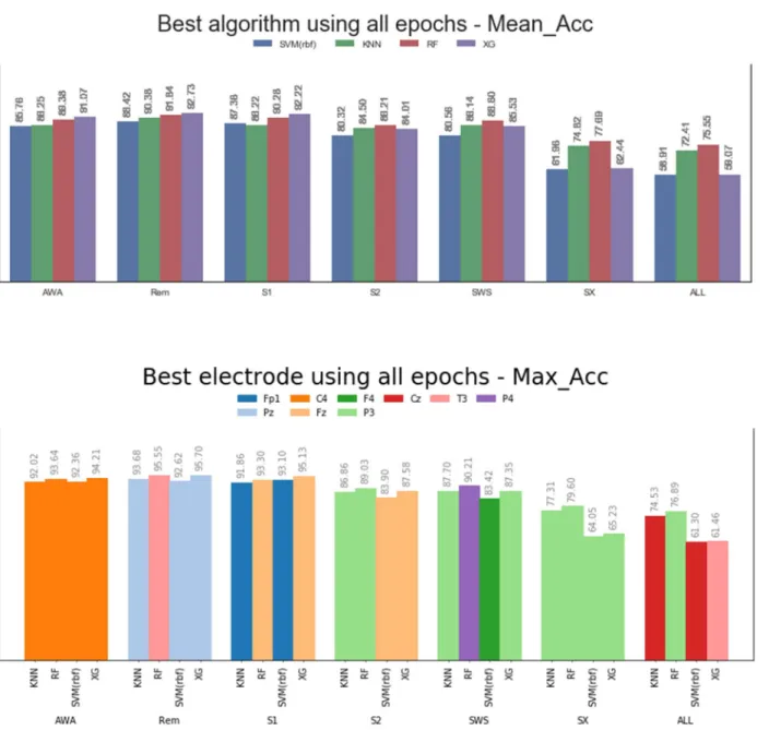
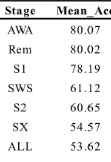
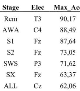
4.1.5 Best algorithm and Best Electrode ... 37
4.2 Undersampling ... 38 4.2.1 Learning curve ... 38 4.2.2 SVM (rbf) ... 40 4.2.3 KNN ... 40 4.2.4 RF ... 41 4.2.5 XG ... 41
4.2.6 Best algorithm and Best electrode ... 42
4.3 Optimization ... 43
4.3.1 SVM (rbf) ... 44
4.3.2 KNN ... 45
4.3.3 RF ... 46
4.3.4 XG ... 47
4.3.5 Best algorithm, Best electrode and Best stage ... 47
4.3.6 Best electrode after optimization – Fp1 vs Fp2 ... 49
4.3.8 Effect of optimization in Fp1 ... 51
4.3.9 Topoplot with RF ... 53
4.3.10 Features importance with RF ... 54
4.4 Benchmark sets: Hold-out, Intruders ... 55
4.4.1 Hold-out set (AWA) ... 55
4.4.2 Hold-out and Intruders set (AWA) ... 57
4.4.3 Continuous identification/authentication (SX-AWA) ... 60
4.4.4 Continuous identification/authentication (ALL – AWA) ... 61
4.5 Discussion and Limitations ... 62
CHAPTER 5 CONCLUSION AND RECOMMENDATIONS ... 66
BIBLIOGRAPHY ... 68
LIST OF TABLES
Table 2-1 : Commercial low-cost headsets ... 7
Table 3-1 : Extracted features ... 21
Table 3-2 : Number of epochs in each dataset ... 24
Table 3-3 : Number of epochs in learning curve – ratio: 90% - 10% ... 26
Table 3-4 : Number of epochs after undersampling ... 26
Table 3-5 : Searching space of hyperparameters optimization ... 30
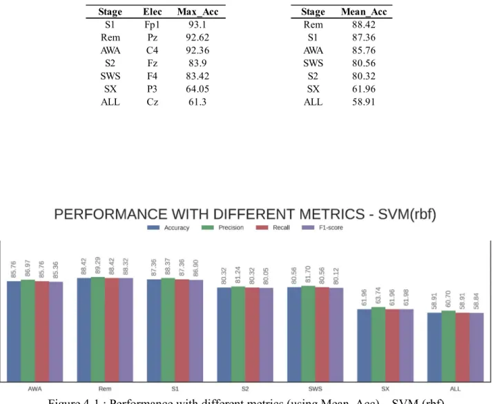
Table 4-1 : Preliminary performance: Best electrode and Best stage – SVM (rbf) ... 33
Table 4-2 : Preliminary performance: Best electrode and Best stage - KNN ... 34
Table 4-3 : Preliminary performance: Best electrode and Best stage - RF ... 35
Table 4-4 : Preliminary performance: Best electrode and Best stage - XG ... 36
Table 4-5: Performance after undersampling: Best electrode and Best stage – SVM (rbf) ... 40
Table 4-6: Performance after undersampling: Best electrode and Best stage – KNN ... 40
Table 4-7 : Performance after undersampling: Best electrode and Best stage – RF ... 41
Table 4-8 : Performance after undersampling: Best electrode and Best stage – XG ... 41
Table 4-9 : Performance optimization: Best electrode and Best stage – SVM (rbf) ... 44
Table 4-10 : Performance optimization: Best electrode and Best stage – KNN ... 45
Table 4-11 : Performance optimization: Best electrode and Best stage - RF ... 46
Table 4-12 : Performance optimization: Best electrode and Best stage - XG ... 47
Table 4-13 : Performance after optimization – RF ... 53
Table 4-14 : Evaluation metrics – Hold-out set_RF ... 56
Table 4-15 : Evaluation metrics – Holdout_Intruders set_RF ... 59
Table 4-16 : Evaluation metrics – Continuous_RF (SX-AWA) ... 60
LIST OF FIGURES
Figure 2-1 : Modules in an EEG biometric system ... 5
Figure 2-2 : a) A 19 electrodes positioning map based on the 10-20 system of a medical grade headset, b) A single Fp1 electrode low cost headset ... 7
Figure 2-3 : Sleep cycles ... 9
Figure 3-1 : Flowchart of biometric model ... 19
Figure 3-2 : Placement of electrodes ... 20
Figure 4-1 : Performance with different metrics (using Mean_Acc) – SVM (rbf) ... 33
Figure 4-2 : Performance with different metrics (using Mean_Acc) – KNN ... 34
Figure 4-3 : Performance with different metrics (using Mean_Acc) – RF ... 35
Figure 4-4 : Performance with different metrics (using Mean_Acc) - XG ... 36
Figure 4-5 : a) Best algorithm – Mean_Acc and b) Best electrode – Max_Acc; preliminary performance (all epochs) ... 37
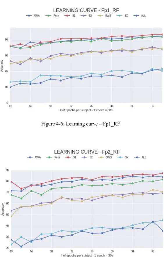
Figure 4-6: Learning curve – Fp1_RF ... 39
Figure 4-7: Learning curve – Fp2_RF ... 39
Figure 4-8 : a) Best algorithm - Mean_Acc and b) Best electrode – Max_Acc; after undersamplig (840 epochs) ... 42
Figure 4-9 : Heatmap : Preliminary optimization on Fp1 and Fp2 – SVM (rbf) ... 44
Figure 4-10 : Heatmap: Preliminary optimization on Fp1 and Fp2 - KNN ... 45
Figure 4-11 : OOB error : Preliminary optimization on Fp1 and Fp2 - RF ... 46
Figure 4-12 a) Best algorithm – Mean_Acc, b) Best electrode – Max_Acc – Mean_Acc; after optimization ... 48
Figure 4-13 : Best electrode after optimization (Fp1 vs Fp2) – RF ... 49
Figure 4-14 : Fp1 (840 + opt) vs Best electrodes per stage (All) - RF... 50
Figure 4-16 : Fp1 (840 + opt) vs Best electrodes per stage (840 + opt) – RF ... 51
Figure 4-17 : Effect of optimization in Fp1 - SVM (rbf) ... 51
Figure 4-18 : Effect of optimization in Fp1 – KNN ... 52
Figure 4-19 : Effect of optimization in Fp1 – RF ... 52
Figure 4-20 : Effect of optimization in Fp1 – XG ... 52
Figure 4-21 : Topoplot after optimization - RF... 53
Figure 4-22 : Hold-out set (4 epochs per subject) – Fp1_RF ... 56
Figure 4-23 : Holdout_Intruders set – Fp1_RF ... 59
Figure 4-24: Continuous authentication - Fp1_RF (SX-AWA) ... 60
LIST OF SYMBOLS AND ABBREVIATIONS
ADD Attention Deficit disorder AWG Arbitrary Waveform Generator AEP Auditory evoked potential AR Autoregressive model DFT Discrete Fourier Transform DTW Dynamic Time Warping ECG Electrocardiography ED Euclidean distance EEG Electroencephalography EER Equal error rate
EMD Empirical Mode Decomposition EMG Electromyography
EOG Electrooculogram ERP Event related potential ERR Error rate
FAR False accept rate
FDA Fisher Discriminant Analysis FFT Fast Fourier Transform FRR False reject rate
HTER Half Total Error Rate HHT Hilbert-Huang Transform HSA Hilbert Spectral Analysis IMF Intrinsic Mode Functions
IoT Internet of things IQR Interquartile range KNN K-nearest neighbour
LDA Linear Discriminant Analysis LVQ Learning Vector Quantizer
MFCC Mel-frequency Cepstral Coefficients
NN Neural Networks
OOB Out-of-bag
PSD Power spectral density PSG Polysomnography REC Resting eyes closed REO Resting eyes opened
RF Random Forest
SE Shannon entropy
SSEP Somatosensory evoked potential SSS Stratified Shuffled Split
SVM Support Vector Machine VEP Visual evoked potential
WPD Wavelet packet decomposition
LIST OF APPENDICES
APPENDIX A – DIFFERENT STUDIES FOR RESTING STATE ... 78
APPENDIX B – DIFFERENT STUDIES FOR SENSORY STIMULI ... 81
APPENDIX C - DIFFERENT STUDIES FOR COGNITIVE ACTIVITIES ... 82
APPENDIX D – FEATURES IMPORTANCE PER ELECTRODE (AWA) ... 83
APPENDIX E - FEATURES IMPORTANCE PER ELECTRODE (SX) ... 84
APPENDIX F: FEATURES IMPORTANCE PER ELECTRODE (ALL) ... 85
CHAPTER 1
INTRODUCTION
Hospitals are crowded as many people go for not emergency causes: chronic diseases, elderly care or small problems like cough, etc. This makes the service unavailable to people who are really in need. Thanks to Internet of Things (IoT) and big data, remote diagnostics and real-time monitoring will be possible.
However, spoofing techniques are becoming more sophisticated, for example: a) Fingerprints can be spoofed by reactivating the print left by the last user (by dusting or breathing on the collection plate), using a special tape with the fingerprint of somebody else, or using prosthetic fingers; b) Faces can be spoofed using 3D masks, high resolution photos or videos and c) Iris can be spoofed using high resolution images or contact lenses. Also, all of these traits are subject to physical damage.
Furthermore, the anti-spoofing measures have a limited validity period because they require careful feature engineering to detect real traits from fake ones. Special attention has been paid to the “liveness detection” measure which works by detecting physiological properties from a living body such as: electroencephalography (EEG), pupil dilatation and blinking. So, to prevent identity fraud by spoofing attacks, EEG has been proposed. As this physiological biometric is not static, it is possible to extract unique features to distinguish subjects. Other advantages over conventional biometrics are: it is “universal” which means that every person alive has them; it can monitor vital signs and emotional states (which could be useful for preventive medicine); and as it can be recorded for long periods in real time, the subject can be identified/authenticated continuously. A lot of research has been done using different types of acquisition protocols: VEP, resting state, and cognitive activities. Many types of features have been used: Fast Fourier Transform (FFT), Wavelet, Correlation, entropy, etc. And also many algorithms: SVM, NN, KNN, LDA, etc. Performance is promising, but technology has not been adopted yet. Some possible drawbacks are: EEG is affected by arousal, attentional states, age and disease. All this variability makes it ideal as the perfect password, as it is unpredictable, but also difficult to manage. In addition, the enrollment (training) and identification/authentication (test) time must be fast for its deployment in real life. Finally, a small number of electrodes (ideally 1) must be capable to identify/authenticate.
1.1 Research Objectives
GENERAL OBJECTIVE
Identify and authenticate persons using their EEG during awake and sleep stages.
Many studies have been done with EEG using different protocols: VEP, resting state (eyes opened and closed) and cognitive activities; but never in subjects during wakefulness, sleep and a combination of them. So, the objective of this research is to examine the potential of EEG data as a reliable biometric tool. The main application could therefore be in the context of telemedicine, which is of increasing interest (easing the load of hospitals by decentralizing resources).
In order to answer to this question, this general objective has been divided in small specific research questions.
SPECIFIC OBJECTIVES
What stage is more efficient for identification/authentication?
From a neuroscience perspective, it is interesting to know in what stage the EEG power distribution is characteristic for an individual and therefore may reflect individual traits of brain morphology that may eventually be used to personalize clinical practices.
Furthermore, as the resting state has been reported as a non-static phenomenon (due to fluctuations in attention), then maybe with a natural recurring state like sleep it could be answered if a brainprint exists.
Is it possible to distinguish individuals using 1 electrode?
This is important as EEG biometrics has to comply with the usability criteria. If too many electrodes are used, then the technology will not be adopted.
What is the minimal duration, in seconds, to identify/authenticate a person?
This objective is inside the usability criteria. Enrollment and identification/authentication time need to be small in order to make the technology fast and therefore easily adopted.
Is there entropy in brain signal?
Previous studies have proposed the use of EEG signals to generate cryptographic keys. In cryptanalysis, entropy is used as a way to measure the unpredictability of a cryptographic key. So, a comparison of the importance of the « spectral entropy » feature against EEG bands was done to answer this question.
What is the effect of hyper-parameter optimization in performance?
Most studies focus on feature engineering. But the performance with novel features has shown to be comparable or worse than the conventional used ones.So instead of looking for more effective features, this research uses a conventional set of features andfocuses on hyper-parameter optimization to boost performance. In addition, the optimization ensures a fair comparison among algorithms when choosing the best performing one.
Is continuous identification/authentication possible?
This form of identification/authentication will be useful to recognize someone regardless of how the brain is engaged during the telemedicine session. In this research, 2 states have been studied: Wakefulness and Sleep.
1.2 Thesis structure
There are 3 chapters in this thesis excluding the Introduction and the Conclusion ones.
Chapter 2 presents advanced concepts related to machine learning, biometrics and neuroscience; and a survey of existing literature related to EEG biometrics. In Chapter 3, the applied methodology and how it was useful to answer the research questions, is described. And finally in Chapter 4, the results are explained.
CHAPTER 2
BIOMETRICS AND MACHINE LEARNING: CONCEPTS
AND LITERATURE REVIEW
2.1 Biometrics
It is a form of identification/authentication and access control which uses human traits to describe individuals (A. K. Jain, Bolle, & Pankanti, 2006).
According to the trait, it can be of three types:
Physiological: Related to the shape of the body. Ex: fingerprints, palm veins, face recognition, DNA, palm print, hand geometry, iris recognition, retina and odour.
Behavioural: Related to behaviour patterns. Ex: typing rhythm, gait and voice.
Of intent: by analyzing physiological features, behaviour can be predicted. Ex: EEG, ECG. The compliance of a particular biometric to a specific application involves several factors:
Universality: every person should possess the trait.
Uniqueness: the trait should be enough different among population to distinguish each one from each other.
Permanence: how the trait varies in time. A good trait should be reasonably invariant over time.
Measurability: ease of trait measurement.
Performance: related to the accuracy, speed and robustness of the technology used to process the trait.
Acceptability: how easy the population accepts the technology. If they are willing to have their trait measured.
2.2 Modules for an EEG biometric system
Depending on the application context, a biometrics system can work in two modes: authentication and identification (A. Jain, Flynn, & Ross, 2008).
Authentication: Used to prevent different people from using the same identity.
A user willing to be recognized claims an identity, usually using a user name. The system performs a one-to-one comparison (captured biometric with stored template) to determine whether the claim is true or not. (Is this the biometric of Alice?)
Identification: It aims to prevent a single person from using multiple identities. The system performs a one-to-many comparison (searching through all stored templates for a match) to determine the identity of an unknown individual (whose biometric data is this one?)
Figure 2-1 : Modules in an EEG biometric system
Figure 2-1 (A. Jain et al., 2008) (Abbas, Abo-Zahhad, & Ahmed, 2015) displays the modules of a biometric system: signal acquisition, preprocessing technique, features extraction and feature classification.
2.2.1 Signal acquisition
The trait used in this research is the Electroencephalography (EEG). The use of electrodes, a specialized headset and a brain stimulus are necessary.
a) Electroencephalography (EEG)
EEG is the recording of the electrical activity of the brain using electrodes placed along the scalp. It measures spontaneous electrical activity of neurons within a period of time (Niedermeyer & Silva, 2004). The amplitude of signals ranges between 10 and 200 uV with a frequency in the range of 0.5 – 100 Hz. The waveforms can be classified into different frequency bands:
Typical EEG bands: delta (< 4Hz), theta (4 Hz – 7 Hz), alpha (8 Hz – 15 Hz), beta (16 Hz – 31 Hz) and gamma (>32 Hz) (Tatum, 2014).
b) Headsets
In Figure 2-2 (Maskeliunas, Damasevicius, Martisius, & Vasiljevas, 2016) (“Neurosky,” 2007), it can be seen the two types of headsets that have been used in biometrics research: a) medical-grade and b) low cost.
Medical-grade: Contains a large number of electrodes usually of the wet type (they need to be moistened by electrolytes). Signals of better quality can be obtained but the setting up for signal acquisition is a shortcoming in biometrics applications.
The distribution of electrodes over the scalp follow the 10-20 system or the 10-10 system (Homan, Herman, & Purdy, 1987). Both are internationally recognized methods to describe the location of electrodes for a test or experiment.
Low-cost: Contains very small amount of electrodes of the dry type. Offers a low signal quality but the setting up for signal acquisition is not complex when compared to medical grade headsets. Table 2.1 shows some commercial low-cost headsets that have been used in biometrics research.
Figure 2-2 : a) A 19 electrodes positioning map based on the 10-20 system of a medical grade headset, b) A single Fp1 electrode low cost headset
Table 2-1 : Commercial low-cost headsets
c) Brain stimulus
It can be classified in 3 acquisition protocols: resting state, sensory (audio/visual) stimuli and cognitive tasks (verbal instructions). Additionally, sleep stages will be described; as they have been used in this study.
Resting state: Subjects are sat on a chair in a quiet environment with either eyes open or closed. They provide EEG signals without any additional instruction. Articles that have used this protocol are presented in Appendix A.
Sensory stimuli: An event related potential (ERP) is a brain response triggered by a ” specific sensory, cognitive or motor event” (Luck, 2005).
Device No. Electrodes Released
Neurosky 1 – DRY 2007
Emotiv EPOC 14 – WET 2009
MindWave 1 – DRY 2011
iFocusBand 1 – DRY 2014
Muse 4 – DRY 2014
OpenBCI 8 or 16 – DRY/WET 2014
Aurora Dreamband 1 – DRY 2015
According to the source of stimuli it can be classified as Visual Evoked Potential (VEP), Auditory Evoked Potential (AEP) and Somatosensory Evoked Potential (SSEP). Until the date only VEP have been used in biometrics research (Del Pozo-Banos, Alonso, Ticay-Rivas, & Travieso, 2014).
The P300 wave belongs to the ERP category. “When recorded by EEG, it surfaces as a positive deflection in voltage with a delay between stimulus and response of 250 to 500 ms” (Polich, 2007).
To obtain a VEP, subjects are instructed to watch a series of pictures. After each picture, the EEG is recorded. P300 can be accurately measured during feature extraction. This makes them an asset for biometric systems. A drawback is the need for external devices to trigger the P300 signals. This results in a more complex system when compared to other protocols. Articles that have used this protocol are presented in Appendix B and (R. Palaniappan & Raveendran, 2002), (Ravi & Palaniappan, 2005), (R. Palaniappan, 2006), (R. Palaniappan & Mandic, 2007). Cognitive activities: It involves asking subjects to perform cognitive tasks during data
collection including: mathematical calculation, geometric figure rotation, mental letter composition or visual counting. Also imaginary movements involving hands, legs, etc. Articles that have used this protocol are presented in Appendix C and (R Palaniappan, 2005).
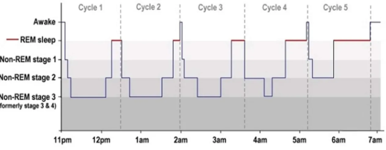
Sleep stages: Sleep scoring is a critical step used in clinical routines to diagnose pathologies such as: insomnia, hypersomnia, circadian rhythm disorders, epilepsy, apnea, etc. Sleep stages can be of 2 types: Rem and Non-Rem. Non-Rem is subdivided in: S1, S2 and SWS (sometimes known as S3). It happens in cycles which go from 90 to 120 minutes. Each cycle follows the following order: S1, S2, SWS; and after a period in SWS it goes back through S2 and S1; then it may enter Rem and a new cycle starts (“How sleep works,” n.d.).
In Figure 2-3 (“How sleep works,” n.d.), the sleep cycle is shown:
A. Rem: This is the rapid eye movement stage. It counts for up to 20 to 25 % of total sleep time in adults.
B. S1: This is a stage between wakefulness and sleep. It usually lasts less than 10 minutes. So, it represents about 5% of the total sleep time.
C. S2: Particular waveforms happen here (Sleep spindles and K-complexes) to suppress any response to outside stimuli. It represents 45 to 50% of total sleep time.
D. SWS (Slow Wave Sleep): This is deep sleep. It represents around 15% to 20% of total sleep time.
Figure 2-3 : Sleep cycles
2.2.2 Feature extraction
The selection of discriminative features is important in any type of classification problem. In EEG biometrics, the extraction of features has been conducted in the time and frequency domain. A review of the most employed methods is provided in this section:
a) Power Spectral density (PSD)
It indicates the spectral density distribution of a signal in the frequency domain. It is computed from the Fourier Transform (FT). But, as EEG signals are non-stationary series; the truncated Fourier Transform 𝑥 (𝜔) over a finite interval [0, T] is computed. The signal is assumed to be stationary within that interval and the PSD 𝑆 (𝜔) of the signal x(t) may be computed. Where 𝑥 (𝜔) is the FT of x(t) (Oppenheim, Schafer, & Buck, 1999).
𝑆 (𝑤) = lim
Articles that have used this method are presented in Appendix A, B, C and (R. Palaniappan & Mandic, 2007), (R. Palaniappan & Raveendran, 2002), (Safont, Salazar, Soriano, & Vergara, 2012), (Nakanishi, Baba, & Miyamoto, 2009).
b) Autoregressive Model (AR)
It is a time domain representation of a random process. It is used to describe time-varying processes such as EEG. As its name suggests, it specifies that the output variable depends linearly on its own previous values and on a stochastic term (Pardey, Roberts, & Tarassenko, 1996).
It is defined as an AR model of order p:
𝑋 = 𝑐 + 𝜑 𝐵 𝑋 + 𝜀
where the signal 𝑋 is represented by a series of AR coefficients 𝜑 , white noise 𝜀 , a constant (c) and a lag operator (B). Articles that have used this method are presented in Appendix A, B, C and (Paranjape, Mahovsky, Benedicenti, & Koles, 2001), (Brigham & Kumar, 2010).
c) Wavelet Packet decomposition (WPD)
It decomposes the signal into both time and frequency representations which provide more information into the feature space (Daubechies, 1992).
It is defined as follows:
𝑊𝑇 {𝑥}(𝑎, 𝑏) = ≺ 𝑥, 𝜓 , ≻= 𝑥(𝑡)𝜓 , (𝑡)𝑑𝑡
Where: 𝑊𝑇 {𝑥}(𝑎, 𝑏) are the wavelet coefficients, x(t) is the time domain signal and 𝜓 . (𝑡) is the wavelet function.
It is applied by multiplying the EEG signal with different wavelet functions, in which each one can have different scale (a) and shift (b) according to specific applications.
Articles that have used this method are presented in Appendix A, B, C and (Abdullah, Subari, Leo, Loong, & Ahmad, 2010).
d) Other methods
Hilbert-Huang Transform (HHT): It is a fairly new algorithm, designed to specifically work with non-stationary and nonlinear signals. As it preserves the characteristics of the varying frequency (N. Huang et al., 1998).
It has two main steps:
1) Uses the Empirical Mode Decomposition (EMD) method to generate the Intrinsic Mode Functions (IMF).
2) Performs the Hilbert Spectral Analysis (HSA) on each IMF to obtain instantaneous frequency data.
Articles that have used this method are presented in Appendix A, B, C and (Kumari, Kumar, & Vaish, 2014).
Euclidean distance (ED) and Dynamic Time Warping (DTW): Employed by (Gui, Jin, Ruiz Blondet, Laszlo, & Xu, 2015), to measure the similarity between two EEG signals. Shannon entropy (SE): (Phung, Tran, Ma, Nguyen, & Pham, 2012) claimed that similar
performance was obtained when compared against AR but much faster speed in identification.
Time domain peak matching algorithm: Novel technique proposed by (Singhal & Ramkumar, 2007).
Equivalent root mean square (rms) values for each electrode signal over a 1 second period: Time domain feature with low computational cost but high performance, proposed by (Altahat, Tran, & Sharma, 2012).
Conventional Mel-frequency Cepstral Coefficients (MFCC): Suggested by (Nguyen, Tran, Huang, & Sharma, 2012). It is usually employed for voice recognition.
2.2.3 Feature classification
A classification scheme is necessary to make predictions. There are many types of algorithms. A brief description of the most popular ones used in EEG biometric is provided as well as the ones used in this research.
a) Algorithms
K-Nearest Neighbour (KNN): It is a lazy learning algorithm because it constructs hypotheses directly from the training set stored in memory rather than generalizing. This makes it sensitive to the class distribution: the more frequent class will dominate the prediction of the tested epochs3. To overcome this, it is a good idea to assign distance
weights so that the closer neighbors are the ones that contribute the most to the final prediction.
It is also sensitive to noisy data, as it uses the distance among epochs to define the belonging to a class. To solve this, it is important to standardize the feature vectors.
An advantage of this algorithm is its ability of adaption to unseen data and its fast classification process: as it only needs the training epochs to be stored together with their respective class labels and be compared with the query epochs directly (Kotsiantis, Zaharakis, & Pintelas, 2006).
Articles that have used this algorithm are presented in Appendix A, B, C and (Ramaswamy Palaniappan & Ravi, 2006), (Yazdani, Roodaki, Rezatofighi, Misaghian, & Setarehdan, 2008), (Su, Xia, Cai, & Ma, 2010).
Kernel methods: Support Vector Machine is one of its best known members who has been found to be competitive with neural networks on tasks such as handwriting recognition (Cortes & Vapnik, 1995).
SVM searches for a hyperplane to separate different classes. This hyperplane has to maximize the margin between different classes to ensure generalization capabilities. Depending on the training set distribution, a non-linear hyperplane might be needed. For this effect a kernel function is required. Some popular examples: polynomial, radial basis function, sigmoid (C.-W. Hsu & Lin, 2002).
3 Epoch: Time window extracted from the continuous EEG signal. It is how the signal has been "chopped" into segments.
By design it is a binary algorithm but several methods have been proposed to extend it to multiclass problems:
A. One-versus-all: It distinguishes between one of the classes and the rest. There is one classifier per class. The one with the highest performance assigns the class. It is computationally efficient (only n_classes classifiers are needed) and interpretable. B. One-versus-one: It distinguishes between every pair of classes. At prediction time, the
class which received the most votes is selected. It is slower than One-versus-all but scales well when using kernel methods (n_classes * (n_classes - 1) / 2).
Articles that have used this algorithm are presented in Appendix A, B, C and (Hu, 2010), (Ashby, Bhatia, Tenore, & Vogelstein, 2011).
Linear Discriminant Analysis (LDA): It can be used as a classifier or as a dimensionality reduction technique. It searches for a linear combination of variables that best separates classes but assumes that all these share the same covariance matrix (McLachlan, 2004). Articles that have used this algorithm are presented in Appendix A, B, C (Lee, Kim, & Park, 2013).
Neural Networks (NN): It is a collection of learning algorithms inspired by the brain's neural networks. It consists of three main layers of nodes (neurons): input, hidden and output; being the hidden layer the only one that varies in number. All these layers are interconnected and the signal propagates from the input to the output. In each node of the hidden layer there is an activation function which only responds to the output of its previous node. The results of these operations are fused and a prediction is made (Duda, Hart, & Stork, 2001). Articles that have used this algorithm are presented in Appendix A, B, C and (R Palaniappan & Mandic, 2005), (Chunying, Haifeng, Lin, & Bing, 2014), (Gui, Jin, & Xu, 2015).
Random Forest (RF): It is a form of ensemble learning. It produces many trees based on a random selection of epochs and random selection of features. Then it predicts classes based on the majority vote of all trees (Breiman, 2001). It has not been used on EEG biometrics.
Extreme Gradient Boosted trees (XG): It is an advanced Gradient Boosted classifier proposed by (Chen & He, 2015). It is very popular among winning solutions in Kaggle's machine learning competitions. It focuses on computational speed and model performance. Models are built sequentially and each one can correct the errors of prior models. Then all models are combined together into a strong one to make a final prediction. It has not been used on EEG biometrics.
2.3 Hyperparameter optimization
Each algorithm, according to its functioning, may or may not possess hyperparameters. The hyperparameters are the parameters that cannot be directly learnt from the dataset and therefore require fixing before model training to control model complexity. There are 2 popular brute-force techniques:
a) Grid search: It is an exhaustive search (and therefore expensive) through a finite set of “reasonable” values for each hyperparameter. It suffers from the curse of dimensionality but its workload can be separated in parallel tasks (Bergstra & Yoshua, 2012).
b) Random search: It works by sampling from a distribution of possible hyperparameter values, where the number of sampled candidates has to be specified. The higher this number is, the finer the search becomes. Frequently, some hyperparameters do not change significantly the algorithm's performance; making random search more effective than grid search in high dimensional spaces (Bergstra & Yoshua, 2012).
2.4 Performance evaluation
In biometrics there are many metrics used to evaluate a system. In this research the following ones have been used (Sokolova & Lapalme, 2009), (West Point Academy, 2012).
a) Accuracy: It is the number of all correct predictions divided by the total number of samples of the dataset. It can also be calculated by 1 – ERR. Its paradox is that for highly unbalanced datasets it will reflect the underlying class distribution. TP is True Positive, TN is True Negative, FP is False Positive and FN is False Negative.
𝐴𝐶𝐶 = 𝑇𝑃 + 𝑇𝑁 𝑇𝑃 + 𝑇𝑁 + 𝐹𝑁 + 𝐹𝑃
b) Precision: Also called Positive Predictive Value. It is the proportion of predicted positives which are actual positive. TP is True Positive and FP is False Positive.
𝑃𝑅𝐸 = 𝑇𝑃 𝑇𝑃 + 𝐹𝑃
c) Recall: Also called Sensitivity or True Positive Rate. It is the proportion of actual positives which are predicted positive. TP is True Positive and FN is False Negative.
𝑆𝑁 = 𝑇𝑃 𝑇𝑃 + 𝐹𝑁
d) F1-score: Also known as balanced F-score or F-measure. It is the harmonic mean between precision and recall.
𝐹1 = 2 (𝑝𝑟𝑒𝑐𝑖𝑠𝑖𝑜𝑛 ∗ 𝑟𝑒𝑐𝑎𝑙𝑙) 𝑝𝑟𝑒𝑐𝑖𝑠𝑖𝑜𝑛 + 𝑟𝑒𝑐𝑎𝑙𝑙
e) Type I Error: Also called False Negative Rate or False Reject Rate. It is when a system rejects access to a legitimate identity. TP is True Positive and FN is False Negative.
𝐸𝑟𝑟𝑜𝑟𝐼 = 𝐹𝑁 𝑇𝑃 + 𝐹𝑁
f) Type II error: Also called False Positive Rate or False Accept Rate. It is the proportion of actual negatives which are predicted as positive. It is when a system grants access to an illegitimate identity. TN is True Negative and FP is False Positive.
𝐸𝑟𝑟𝑜𝑟𝐼𝐼 = 𝐹𝑃 𝑇𝑁 + 𝐹𝑃
g) HTER: Half Total Error Rate. It is an aggregate of FAR and FRR. Most authentication systems are measured and compared using HTERs or variations of it.
𝐻𝑇𝐸𝑅 = 𝐸𝑟𝑟𝑜𝑟𝐼 + 𝐸𝑟𝑟𝑜𝑟𝐼𝐼 2
2.5 Previous work and current limitations
In this section previous works are compared and analysed. This serves to give a comprehensive review of what has been done and also to justify the chosen methodology for this research. For EEG to be considered a successful biometric technology, it has to satisfy two conditions: 1) Reliable recognition performance and 2) Usability: number of electrodes, location of electrodes, duration of training set (enrollment) and test set (recognition).
As the number of electrodes is an important condition for usability and the studied database consists of wakefulness and sleep stages; only works that have used 1 electrode (wet or dry) in resting state will be discussed. For a review of other works using different number of electrodes or other types of brain stimulus check Appendix A, B and C.
The first series of related works started in 1998 by (Poulos, 1999). Their work is based on the findings by (Vogel, 1970) about the inheritance of EEG traits. A dataset of 4 genuine users and 75 intruders in resting state with eyes closed (REC) was used. The proposed methodology fitted a linear model of the AR type on the alpha rhythm recorded by the O2 electrode and classified it by a Computational Geometry algorithm (convex polygon intersections). It reached a 95% success rate on classification. However, the fact that the dataset contained only 4 subjects prevents to make a final conclusion.
In a future work, (Poulos, Rangoussi, Alexandris, & Evangelou, 2002) used all the main brain bands (alpha, beta, delta, theta), on that same dataset. But this time using a bilinear model to extract features; prompted by an already investigated conjecture of the existence of non-linear components in EEG; and the use of a Learning Vector Quantizer (LVQ) neural network for classification. An accuracy of 99.5% was obtained.
(Paranjape et al., 2001) tested a dataset of 40 subjects in REO and REC states. The methodology also used an AR type model on the alpha rhythm for feature extraction, but on the P4 electrode. As
a classifier, a Linear Discriminant was employed reaching an impressive 99% in accuracy when all dataset was used and 85% when partitioning the dataset. Even though the 99% performance might be due to overfitting the data; the obtained accuracy of 85% when partitioning the dataset is still impressive and proved that the identification of subjects by means of EEG is possible. In 2010, (Su, Xia, Cai, Wu, & Ma, 2010) published a study using a low cost headset with an Fp1 electrode, in which it was addressed the effects of diet and/or circadian rhythms. The dataset consisted of 40 subjects in REC where AR coefficients and PSD from 5 to 32 Hz features were extracted. Three classifiers were tested, but it was the combination of Fisher Discriminant Analysis (FDA) and KNN that reached a 97.5% when all dataset was used (without constraints of diet or circadian rhythm).
(Zhao et al., 2010) also employed a low cost headset but with an electrode in Cz; to record a dataset of 10 subjects in REC. A 97.63% was reached using KNN and linear features. These results are a contradiction because (Poulos et al., 2002) demonstrated that non-linear features were better suited for EEG biometrics. It is possible that the used algorithm (Neural Networks) has influenced the difference in results.
Finally, (Dan, Xifeng, & Qiangang, 2013) compared 3 algorithms: SVM, LDA and NN also using a low cost headset with an electrode in Fp1. The best performance was of 87% with SVM and AR features.
What all these works have in common is a high performance (over 80%), the use of a single electrode (wet or dry) in different brain locations, the continuous search for better features to discriminate among subjects and the many types of algorithms to perform classification. But there are no details whether hyperparameter optimization has been done. And this is an important step to control model complexity and to do a fair comparison among algorithms. According to (Yang, 2015) and by inspecting the Appendix A, B and C; the performance with novel features is comparable with the conventional ones (AR coefficients and PSD) or worse. So instead of looking for more effective features, this research focuses on hyperparameter optimization to boost performance, and to study the effect of reducing the number of epochs to make the biometrics system faster.
Determined by neurophysiology, brain rhythms occur in different brain regions according to the stimulus. Under the REC condition the occipital, temporal and parietal areas are the ones providing
the most discriminative information (Campisi et al., 2011), (Rocca, Campisi, & Scarano, 2012), (Parisa, Mo, & Mohammad, 2006). Meanwhile, under REO anterior brain regions are implicated (Bear, M; Connors, B; Paradiso, 2014), (Abdullah, Subari, Leo, et al., 2010), (Abdullah, Subari, Loong, & Ahmad, 2010), (P Tangkraingkij, Lursinsap, Sanguansintukul, & Desudchit, 2009), (Preecha Tangkraingkij, Lursinsap, Sanguansintukul, & Desudchit, 2010). But this represents a problem for the deployment of EEG biometrics as it does not comply with the usability criteria. Users have to see EEG biometrics as an unobtrusive option to monitor and improve their health. So, instead of using a brain region that is best for the stimulus, one that is best for the user was chosen: the frontal lobe. The advantage of this region is that the difficulty of applying electrodes correctly to the scalp and the reduced performance for individuals with long or coarse hair is almost nonexistent (Mihajlovic, Grundlehner, Vullers, & Penders, 2015), (David Hairston et al., 2014), (Ekandem, Davis, Alvarez, James, & Gilbert, 2012).
All EEG recordings are affected by muscle (frequencies > 20 Hz) (Muthukumaraswamy, 2013) and EOG artifacts (Urigüen & Begoña, 2015), (Schlögl et al., 2007). So, the innovative of this approach is that EEG electrodes in the frontal lobe are usually not taken seriously for the reasons mentioned before, even after removing the artifacts by software. But by focusing on the algorithm rather than on the features, I want to prove that classification performance can be increased without losing in usability. Therefore, the electrodes in this region are going to be tuned by performing hyperparameter optimization, and compared against the ones in the best region for the stimulus. Many studies have focused on EEG as a potential biometric technology. Many brain stimuluses have been tested, each one with its advantages and disadvantages. VEP needs an external device to elicit ERP. Cognitive activities are not feasible for everyone; ex: Attention Deficit disorder (ADD) or handicapped patients. Meanwhile, a resting state is quite easy for everybody. Nevertheless, there are some studies which consider it a dynamic state, due to the fluctuations in attention (Gonçalves et al., 2006), (Laufs et al., 2003), (Stark & Squire, 2001) as humans cannot be just forced to think about nothing. And it is this dynamic that possibly influences the variability across subjects and therefore explains the high rates in performance. In contrast, “Sleep is a naturally recurring state of mind and body, characterized by altered consciousness, relatively inhibited sensory activity, inhibition of nearly all voluntary muscles, and reduced interactions with surroundings” (American Academy of Neurology, 2012). Then maybe with sleep states it could be answered if a real brainprint exists.
CHAPTER 3
METHODOLOGY AND MATERIALS
A full night raw database of wakefulness and sleep EEG recordings was used. Signal pre-processing techniques were applied to remove noise and create five datasets: AWA, Rem, S1, S2, SWS. The same features used in (Lajnef et al., 2015) were extracted for each of the 19 electrodes, and two additional datasets were created (SX, ALL) which are a combination of the other stages. So, 19x7 datasets were studied in this experiment. In order to test identification/authentication capabilities, all these datasets were split in Legitimates, Intruders and Hold-out sets. Assignment of subjects to these sets was based on the availability of sufficient number of epochs across the various stages. More details are given in Step 2 of Figure 3.1.
Firstly, four algorithms were used to get a preliminary classification performance: Support Vector Machine (rbf), K-nearest neighbour, Random Forest and XGBoost only on the Legitimates datasets. Secondly, a removal of epochs4 was done to reduce training and testing duration. And, the
previously mentioned algorithms were once more used to evaluate changes in performance. Finally, all algorithms were optimized and the most performing one was chosen to be tested against the Intruders and Hold-out sets.
Figure 3-1 : Flowchart of biometric model
4 Epoch: Time window extracted from the continuous EEG signal. It is how the signal has been "chopped" into segments.
Data analysis and visualization: feature extraction until permutation test were done using Python 3 and Scikit libraries. Data format conversions were performed with in-house software package for electrophysiological signal analysis (ELAN) developed at INSERM U1028, Lyon, France (Aguera, Jerbi, Caclin, & Bertrand, 2011).
3.1 Raw data
One full night of polysomnographic (PSG) recordings in 38 healthy subjects aged 29.2 +/- 8 years was collected at the DyCog Lab of the Lyon Neuroscience Research Center (Lyon, France). Each recording consists of EOG, EMG and 19 scalp EEG channels; positioned according to the international 10-20 system (See Figure 3-2 (Maskeliunas et al., 2016)). A sampling frequency of 1000Hz was used (Eichenlaub, Ruby, & Morlet, 2012). For this research, only the EEG channels were used.
Figure 3-2 : Placement of electrodes
3.2 Biometric model steps
Step 1. Signal preprocessing
Cleaning and feature extraction (Lajnef et al., 2015)
The acquired polysomnographic signals were processed as follows:
Filtering with cut-off frequencies at 0.2 and at 40Hz to minimize the effect of artefacts Segmentation into 30s epochs, according to sleep scoring standards
In total 20 features were computed from each electrode giving a matrix of Nx20, where N is the number of epochs in each class.
Relative spectral power (5), Power ratios combinations (14) and Spectral entropy were calculated from the power spectral density estimation (PSD).
Table 3-1 : Extracted features
The Welch's averaged periodogram method was applied for this purpose (Oppenheim et al., 1999). So, each epoch was divided into 6 non-overlapping segments to which a Hamming window was applied. Then, by averaging these segments, the final power spectral density was obtained.
a) Relative spectral power: It represents what percentage of the signal is made up of oscillations. So, for a particular EEG band it is the absolute power divided by the sum of powers across the other frequencies bands. The absolute power is the sum of the power values within that particular band.
b) Power ratios combinations: These are the combinations of power in the EEG bands: delta (0.5 – 4.5 Hz), theta (4.5 – 8.5 Hz), alpha (8.5 – 11.5 Hz), sigma (11.5 – 15.5 Hz) and beta (15.5 – 32.5 Hz).
c) Spectral entropy: Measures data complexity or how predictable it can be in the frequency domain. It is based on the Fourier transform and calculated according to the Shannon entropy. It was computed from the relative power (Nunes, Almeida, & Sleigh, 2004), (Tsinghua University Press & Sun, 2016).
0. relPowDelta 7. powDelta/powAlpha 14. powAlpha/powTheta 1. relPowTheta 8. powDelta/powBeta 15. powAlpha/powBeta 2. relPowAlpha 9. powDelta/powSigma 16. powAlpha/powSigma 3. relPowBeta 10. powTheta/powDelta 17. powBeta/powTheta 4. relPowSigma 11. powTheta/powAlpha 18. powBeta/powSigma 5. SpectralEntropy 12. powTheta/powBeta 19. powSigma/powTheta 6. powDelta/powTheta 13. powTheta/powSigma
Step2. Datasets Preprocessing Creation and standardization
The five datasets (AWA, Rem, S1, S2, SWS) were inspected and two additional datasets were created: SX, ALL. The former is the combination of all sleep stages (Rem, S1, S2, SWS); meanwhile the latter is the combination of all sleep stages with wakefulness (AWA, Rem, S1, S2, SWS).
According to the number of epochs some subjects were completely removed meanwhile others were chosen to become part of the Legitimates and the Intruders sets.
Subjects in the Legitimates and Intruders sets, were not chosen randomly. Assignment was based on the availability of sufficient number of epochs across the various stages. To determine who was going to belong to the Legitimates set: a 90-10% sss cross validation ratio was evaluated with different combinations in number of subjects. At the end, a balance between the number of subjects and algorithm performance was found with 21 subjects with over 44 epochs in each stage. The rest (16 subjects) belongs to the Intruders set. “More subjects mean lower performance (more classes makes the classification problem more difficult). Less subjects mean higher performance (the classification problem is easier but the biometric system is not “real”).”
To see the total number of available epochs of these 2 sets, see Table 3.2.
Intruders (16 subjects): The Intruders were never used during training, as they do not have permission to access the system.
Legitimates (21 subjects): The Legitimates have access to the system. So they were used to train the model. From this set, 1 additional subset was created: Hold-out.
A. Hold-out: To create it, 4 epochs were randomly5 removed from each subject. This subset
was used to test the generalization capabilities of the final model; and therefore it had never been used during the model training.
5 Random removal: The ideal way is to use data from the same subject on a different day and training session to take
into account the inter-session variability. As the closer the epochs in time, the more similar they are. However, this does not apply to the Intruders as these subjects do not have access to the system.
The Hold-out and Intruders sets were never used during training and therefore they were used for benchmarking.
Distance and margin based classifiers, such as KNN and SVM respectively, are dependent on feature standardization. Meanwhile tree-based ones, such as RF and XG aren't. But for model comparisons a robust scaler was applied on all datasets.
The robust scaler ensures that outliers do not affect the data standardization. So instead of using the mean and variance; it uses the median and the interquartile range (IQR) on each feature. The IQR is a measure of variability based on dividing a dataset into four equal parts (“RobustScaler,” n.d.).
Step 3. Preliminary Classification
This step is applied only to the Legitimates set.
Even though the datasets of the legitimate users had different number of epochs per subject and stage; 4 algorithms (SVM-rbf, KNN, RF and XG) were tested to get a preliminary performance estimation. As Accuracy can be misleading in datasets with large class imbalance (Machine Learning Mastery, n.d.), additional metrics were used: Precision, Recall and F1-score.
A 10 repetitions of 10 (10x10) stratified shuffled split (sss) cross validation was used to partition each dataset into a 90%-10% ratio for training and testing. This type of cross validation guarantees that classes are uniformly distributed in each partition and that the epochs from each one are not sorted.
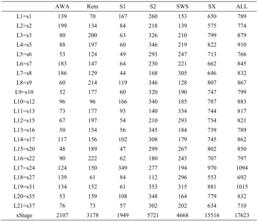
Table 3-2 : Number of epochs in each dataset
LEGITIMATES
AWA Rem S1 S2 SWS SX ALL
L1=s1 139 70 167 260 153 650 789 L2=s2 199 134 84 218 139 575 774 L3=s3 80 200 63 326 210 799 879 L4=s5 88 197 60 346 219 822 910 L5=s6 53 124 49 293 247 713 766 L6=s7 183 147 64 230 221 662 845 L7=s8 186 129 44 168 305 646 832 L8=s9 60 214 119 346 128 807 867 L9=s10 52 177 60 320 190 747 799 L10=s12 96 96 166 340 185 787 883 L11=s13 73 177 93 140 334 744 817 L12=s15 67 197 54 210 293 754 821 L13=s16 50 154 56 345 184 739 789 L14=s17 117 156 102 308 179 745 862 L15=s20 48 189 47 299 267 802 850 L16=s22 90 222 62 180 243 707 797 L17=s24 124 150 349 277 194 970 1094 L18=s27 139 61 84 112 296 553 692 L19=s31 134 152 61 353 315 881 1015 L20=s35 53 159 108 348 164 779 832 L21=s37 76 73 57 302 202 634 710 xStage 2107 3178 1949 5721 4668 15516 17623 INTRUDERS
AWA REM S1 S2 SWS SX ALL
I1=s4 40 144 37 232 207 620 660 I2=s11 20 125 114 342 306 887 907 I3=s14 24 182 46 270 209 707 731 I4=s18 16 181 31 262 291 765 781 I5=s19 37 176 19 191 277 663 700 I6=s21 29 250 35 335 218 838 867 I7=s23 20 214 16 201 335 766 786 I8=s25 35 238 52 352 243 885 920 I9=s26 39 170 60 354 230 814 853 I10=s28 13 156 11 316 327 810 823 I11=s29 10 243 13 327 335 918 928 I12=s30 24 210 39 285 343 877 901 I13=s32 21 159 91 353 198 801 822 I14=s33 109 206 21 330 202 759 868 I15=s34 16 187 54 354 256 851 867 I16=s38 63 129 27 348 231 735 798 xStage 516 2970 666 4852 4208 12696 13212
Step 4. Undersampling
Learning curve6, Random sampling and Model training
A stratified random sampling was used. It consists on randomly removing the same number of epochs from each subject. This is important not only to balance each dataset and make fair comparisons among subjects and stages, but also to reduce training duration (enrollment).
To determine the minimum number of epochs for training, a learning curve has been plotted. This type of plot is an asymptotic analysis to describe limiting behaviour. It shows how better the model becomes as the number of epochs increases in both training and testing sets while keeping the 90-10% ratio and the 10x10 sss cross validation.
A limitation in the datasets was the different number of epochs in each sleep stage and subject. So the learning curve was also limited to both of them. AWA and S1 datasets are the ones with the fewest number of epochs.
Many partitions’ ratios for training and testing were evaluated: 90%-10%, 80%-20% and 70%-30%; even a One-sample-out cross validation. In order to simplify the biometric system and give every subject and stage the same chance while being classified, the total number of epochs for a ratio of 90%-10% must be a multiple of 10 to ensure that each subject will have the same number of epochs during training and testing for each stage. For example, in Table 3.3 when 38 epochs per subject are used this makes: 718 epochs for training and 80 epochs for testing. So, 17 subjects will be tested with 4 epochs meanwhile 4 subjects with only 3 (17x4 + 4x3 = 80). This does not happen if 40 epochs per subject are used (21x4=84).
So, a good balance was found in 40 epochs: 36 for training and 4 for testing. Legitimates: 40 random epochs x 21 subjects = 840 for each stage Intruders: 4 random epochs x 16 subjects = 64 for each stage
Hold-out: 4 random epochs x 21 subjects = 84 for each stage (same size as the test set during cross validation)
6Learning curve: In machine learning it is useful for many purposes. For example: adjusting optimization to improve convergence or comparing different algorithms. In this research, it has been used to determine the amount of data used for training and testing.
And once more, the previous algorithms were tested to check how performance was affected with a reduced number of epochs.
Table 3-3 : Number of epochs in learning curve – ratio: 90% - 10%
LEARNING CURVE: SUBJECTS=21, RATIO=90%-10% # epochs x subject Total Train Test
10* 210 (10) 189 (9) 21 (1) 12 252 226 26 14 294 264 30 16 336 302 34 18 378 340 38 20* 420 (20) 378 (18) 42 (2) 22 462 415 47 24 504 453 51 26 546 491 55 28 588 529 59 30* 630 (30) 567 (27) 63 (3) 32 672 604 68 34 714 642 72 36 756 680 76 38 798 718 80 40* 840 (40) 756 (36) 84 (4)
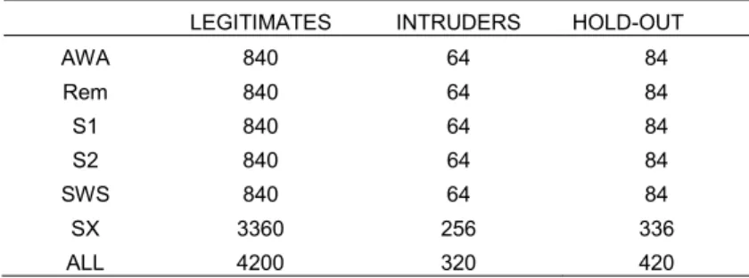
Table 3-4 : Number of epochs after undersampling
LEGITIMATES INTRUDERS HOLD-OUT
AWA 840 64 84 Rem 840 64 84 S1 840 64 84 S2 840 64 84 SWS 840 64 84 SX 3360 256 336 ALL 4200 320 420
Step 5. Optimization
As performance was reduced after undersampling, within all algorithms, a hyperparameter optimization was used to increase it. The hyperparameters are the parameters that cannot be directly learned from the dataset and therefore require fixing before model training to control model complexity.
A random search (RS) strategy was used, as according to (Bergstra & Yoshua, 2012), it is more efficient at finding better models within a small fraction of the computation time, than trials on a grid search. It works by sampling from a distribution of possible parameter values, where the number of sampled candidates is specified. The higher this number is, the finer the search becomes. The identification of the best hyperparameters was performed at each fold using a nested cross validation technique, to avoid the risk of leaking information to the algorithm and therefore overfitting. So, in the inner loop the best hyperparameters combination was chosen, and in the outer loop its performance was evaluated. To partition the datasets, a stratified shuffled split cross-validation method was used.
19x7 final models (one for each electrode and from each dataset) were created. They were used to determine the best sleep stage, best electrode for each stage, the features importance, to make a topographic map of the brain and to test performance against the benchmark sets.
a) Support Vector Machine (SVM): SVM searches for a hyperplane to separate different classes. This hyperplane has to maximize the margin between different classes to ensure generalization capabilities. Depending on the training set distribution, a non-linear hyperplane might be needed. For this effect a kernel function is required. Some popular examples: polynomial, radial basis function, sigmoid (C. W. Hsu, Chang, & Lin, 2016).
As an rbf kernel has been used, the hyperparameters tuned were: C: Penalty parameter. It determines the size of the margin.
gamma: Kernel coefficient. It determines how wiggly the decision boundary becomes. By taking into account the influence of a single sample (far or close).
b) K-nearest neighbor (KNN): KNN defines the class of an epoch by the majority vote of its closest neighbors (Kotsiantis et al., 2006).
The tuned hyperparameters were:
metric: it quantifies the similarity (distance) among epochs to define the belonging to a neighbourhood. Some examples: Euclidean distance, Minkowski distance, Manhattan distance, Cosine similarity and Correlation distance.
n_neighbours: number of neighbour epochs required to vote the class membership of another epoch.
Weight: assigns a weight to the epochs in a neighbourhood. The closer the epochs, the higher their weights.
A coarse random search of 25 parameters combinations was done, as a preliminary optimization step, on the ALL datasets using a 5x5 nested stratified shuffle split. Then a finer search of 20 parameters combinations on all the datasets was applied.
c) Random Forest (RF): It is a form of ensemble learning. It produces many trees based on a random selection of epochs and random selection of features. Then it predicts classes based on the majority vote of all trees.
Usually it is thought that RF does not need hyperparameter optimization, but it does according to (B. F. F. Huang & Boutros, 2016).
The tuned hyperparameters were:
n_estimators: This is the number of trees to be used for the prediction of classes. The bigger the number the more stable the prediction becomes. But the computation time increases. max_features: This is the number of random features used to split each tree.
According to (Breiman, 2001), (Breiman & Cutler, n.d.), it is recommended to use the Out-of-bag score (OOB) to find an optimal range for both hyperparameters. The OOB score is a fast and accurate estimation of the classifier performance without the need of an independent test set.
So an OOB score calculation with the ALL datasets was done to estimate the range of these two hyperparameters. Then a finer random search of 90 parameters combinations, using these ranges, was done on all the datasets.
d) XGBoost (XG): It is an advanced Gradient Boosting classifier proposed by (Chen & He, 2015). It is very popular among winning solutions in Kaggle's machine learning competitions. As it focuses on computational speed and model performance. It builds models sequentially. The new created models can correct the errors of prior models and then all of them are combined together into a strong one to make a final prediction.
The tuned hyperparameters were:
n_estimators: it is the number of trees.
max_depth: it is the pruning of each tree. Unlike RF, in XG large trees easily overfit. learning_rate: Makes the model more robust when generalizing. It reduces the weights at
each iteration.
colsample_bytree: This is similar to max_features in RF. It chooses randomly a number of features.
As the trees are correlated, the OOB error is not a reliable estimation to tune hyperparameters in XG (“XGBoost - Add Out-of-Bag performance validation #1070,” n.d.).
So, a coarse random search of 20 parameters combinations was done, as a preliminary optimization step, on the ALL datasets using a 5x5 nested stratified shuffle split. Then a finer search of 90 parameters combinations on all the datasets was applied.
Table 3-5 : Searching space of hyperparameters optimization
Step 6. Permutation
In order to know if the best performing algorithm was appropriate for the classification task (if the classification score was significant) a standard Permutation test was used (Good, 1994).
In this test, the null hypothesis assumes that the features and the labels are independent p(X,y)=p(X)p(y). To evaluate this hypothesis, the labels were permuted 1000 times; and for each permutation the classification pipeline was executed again.
The obtained p-value is the percentage of runs for which the permutation score was greater than the classification score obtained in the first place. As it was lower than 1/1000, the null hypothesis was rejected. This means that features and classes are dependant and that the algorithm was capable of finding a predictive structure between them.
Model Parameter Preliminar RS Final RS SVM (rbf) C (Penalty)Gamma e-10 -> e10e-10 -> e3 e2 -> e6e-3 -> 1
Model Parameter Preliminar RS Final RS
Knn
n_neighbors 2, 3, 5, 7, 10 2 -> 6 weights distance distance
metric
Model Parameter Preliminar RS Final RS n_estimators 10 -> 400 170 -> 300 max_features 2, 5, 10, 15, 20 5 -> 20
Model Parameter Preliminar RS Final RS XGBoost
n_estimators 100 -> 1000 300 -> 700 max_depth 3 -> 10 6 -> 10 learning_rate e-3 -> e-1 e-2 -> e-1 Colsample_bytree 0.5 ->1 0.5 ->1 minkowski, euclidean, manhattan, cosine, correlation euclidean, manhattan, cosine Random Forest