1
Low Flow Frequency analysis of three rivers in Eastern
Canada
By
Deepti Joshi, André St-Hilaire
Statistical Hydroclimatology Research Group
Institut National De la Recherche Scientifique
Centre Eau, Terre et Environnement
(INRS-ETE)
490 Rue de la Couronne
Québec G1K9A9
2
Contents
1. Introduction ... 3
2. Low flow frequency analysis ... 5
2.1 HYFRAN-PLUS (Hydrological frequency analysis PLUS) ... 5
3. Area of Application... 8
4. Flow Duration curves ... 9
5. Low flow Frequency Analysis ... 12
6. Partial Duration Series ... 15
7. Fitting distribution ... 17
7.1 Method of maximum likelihood ... 18
7.2 Method of Moments ... 19
8. Conclusion ... 30
3
1. Introduction
With an increased attention towards surface water management, information about the estimates of d day, T year low flows are routinely required for the maintenance of water quality standards. Such statistics describing low flows are commonly used in waste load allocation, waste treatment plants, issues governing minimum downstream release requirements for irrigation, hydropower and water supply, etc.
Low flow information can be quantified in a variety of ways depending on the type of data available and the output information desired. Low flow frequency analysis (LFFA) is a stochastic approach for characterising low flow events. The main objective is to ascertain the likelihood that the flow at a particular site will persist below a particular level (threshold) over a particular duration. A flow duration curve (FDC) is one of the most informative ways of displaying the complete range of river discharges from low flows to floods. It gives a relationship between a discharge value and the percentage of time this discharge is equaled or exceeded. Unlike the FDC, a low flow frequency curve (LFFC) shows the percentage of time the flow in a river falls below a given discharge. A LFFC can be constructed for annual minima and minima of 1, 3, 7, 10, 15, 30, 60, 90, 120, 150, 180 days (Smakhtin, 2001). Numerous indices can be obtained from the LFFC. Among the most commonly used ones are the quantiles of the lowest mean discharge over a continuous period of d days corresponding to a recurrence interval of y-years. In Canada, the indices are widely used in water supply systems and waste load allocation (Ouarda et al., 2008). From the perspective of LFFA, the available flow records are
4
generally insufficient for reliable quantification of extreme low flow events and as a result frequency analysis relies on different types of theoretical distribution functions to extrapolate beyond the limits of observed values and to ameliorate the accuracy of low-flow estimation. The „true‟ probability distributions of low flows are unknown and the practical problem is to identify a reasonable „functional‟ distribution and estimate its parameters. In low flow frequency analysis, the most commonly used distributions are Weibull, Gumbel, LogNormal, Gamma, Pearson type-III and log-Pearson type-III (Matalas, 1963; Vogel and Kroll, 1989; Kroll et al., 2002). According to Smakhtin (2001) a universally accepted distribution for low flow analysis is unlikely to be identified. A number of commercial software packages are available (HYFRAN; distribution fitting toolbox, MATLAB) for fitting statistical distributions to the data sample The worked example shown in the report applies some of the low flow frequency analysis techniques to flow data from river Ouelle in Eastern Canada. River Ouelle covers a watershed area of 795 km2 and exhibits more severe summer flows. HYFRAN-PLUS and MATLAB are used to fit statistical distributions to the considered flow data.
5
2. Low flow frequency analysis
The following algorithm outlines the various stages involved in LFFA are shown below:
2.1 HYFRAN-PLUS (Hydrological frequency analysis PLUS)
HYFRAN-PLUS tool is software used to for statistical analysis of sample data. Details about the software can be obtained from
http://www.wrpllc.com/books/HyfranPlus/hyfranplusdescrip.html. The data analysis window (Figure 1) comprises of five tabs:
Derive the low flow time series (Eg: annual, 7 day minima) Test for independence, stationarity
and homogeneity
Derive a frequency curve using plotting position estimates
Distribution fitting and parameter estimation
Comparison of fitted distributions
6
Description: Describing the data name, units, return period definition and empirical probability formula
Data: Data display with identifier and empirical probability calculated on the basis of the selection made in the precious tab.
Basis Statistics: Calculates the mean, maximum, minimum, median, standard deviation, coefficient of skewness and kurtosis
Hypothesis Tests:
Test for Independence (Wald Wolfowitz) Test for Stationarity (Mann Kendall)
Graphics: Observations on probability plot, histogram
7
The following statistical distributions are available Exponential (E)
Generalized Pareto(GP)
Generalised Extreme Value (EV) Gumbel (EV1)
Weibull (2 parameters)
Halphen type A (HA), Halphen type B (HB), Halphen type Inverse B (HIB) Normal
Lognormal 2 (LN2) and 3 parameters (LN3) Gamma (G)
Generalized Gamma (GG) Inverse Gamma (IG) Pearson type 3 (P3) Log Pearson type 3 (LP3)
Compound Poisson exponential (CPE) The criteria for selecting the best fit are:
AIC
where k is the number of parameters in the statistical model, and L is the maximized value of the likelihood function for the estimated model.
BIC
Where n is the number of data points (sample size) Graphical
8
3. Area of Application
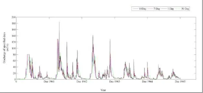
The worked example is based on the discharge station located on river Ouelle. This river is located on the south shore of the St Lawrence River, covering a drainage area of 795 km2. The flow regime of river Ouelle is shown in the following figure (Figure 2). For this river, higher summer temperatures, high summer evaporation and lesser sustained summer groundwater influx are hypothesized to lead to more severe low flows than average for Québec rivers in summer. For this report, daily flow discharge from 1961 to 2010 (46 years after excluding 1967, 1981, 1982 and 1996 due to the presence of missing values) are used.
Figure 2: Mean specific hydrograms for Ouelle. The dotted lines indicate daily mean specific flow plus and minus the daily standard deviation
9
4. Flow Duration curves
Flow duration curves (FDC) give a relationship between magnitude and frequency of streamflow discharges. The data values are first ordered by size. The largest value is given rank 1, the second largest a rank 2 and so on until the lowest has a rank equal to N, the total number of data points. If the two values are equal, they should be assigned different ranks. A plotting position is assigned to each data using a plotting formula. Theoretically, the largest flood should plot at 0 (there would be no chance of it ever being exceeded) and the smallest at 1 (every flood would be equal to or greater than this value). Some of the commonly used probability position formulae includes Weibull (Dairymple, 1960), GEV (using probability weighted moments to estimate generalized extreme value distribution parameters; Hosking et al., 1985) and Cunane (Cunane, 1978). For this report, Cunane plotting position (Cunane, 1978) formula is used. The probability of exceedence and the average recurrence interval calculated using Cunane formula, given by:
and (for floods) and (for droughts)
where N=numbers of years of record, m=rank of the event and .
FDC can be constructed for different time periods: annual, monthly and daily. These curves constructed for daily time series enable a detailed examination of the duration characteristics of a river. For curves constructed for n-day and n-month average flow time series, moving average approach is used. From the perspective of low flows, the section of FDC below median flow
10
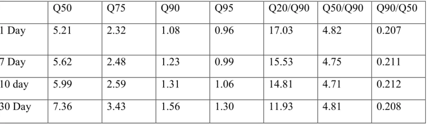
(Q50; discharge equaled or exceeded 50% of the time) is considered vita (Smakhtin, 200l). This section represents groundwater contribution to streamflow from subsurface storages. Various low flow indices can be obtained from this part of the curve. Flows with 70-99% exceedence are widely used as design low flows, ratios Q20/Q90, Q50/Q90 and its reverse Q90/Q50 are also used in low flow studies (Smakhtin, 2001).
Figure 3 and 4 show flows and FDC constructed for 1, 7, 10 and 30 day moving discharges (river Ouelle; 1961-1965). It can be seen that averaging reduces random variations in the data, leading to reduction in peaks and slight increase in low flows. Similar observations can be made from Figure 4, where marked differences between the FDCs can be observed in the high flow region against the low flow section of the curves. The magnitude of flows equaled or exceeded 95% of the time (Q95) obtained from 1,7,10 and 30 day FDCs, shown in Figure 4, are 0.96, 0.99, 1.06 and 1.30 respectively. Some of the indices obtained from the FDCs are shown in Table 1. A reduction in streamflow variability is apparent from the decrease in the values of Q20/Q90. The variability in low flow discharges (Q50/Q90) and proportion of streamflow origination from ground water stores (Q90/Q50) is same for all the FDCs.
11
Figure 3: 1, 7, 10 and 30 day moving averages for a period of 5 years (1961-1965)
12
Table 1: Indices obtained from FDCs obtained using 1, 7, 10 and 30 day moving discharges Q50 Q75 Q90 Q95 Q20/Q90 Q50/Q90 Q90/Q50 1 Day 5.21 2.32 1.08 0.96 17.03 4.82 0.207 7 Day 5.62 2.48 1.23 0.99 15.53 4.75 0.211 10 day 5.99 2.59 1.31 1.06 14.81 4.71 0.212 30 Day 7.36 3.43 1.56 1.30 11.93 4.81 0.208
5. Low flow Frequency Analysis
Low flow frequency curves are a graphical means of understanding the characteristics (frequency, duration and magnitude) of low flow events. LFFC can be constructed on the basis of annual flow minima (daily or monthly minimum discharges) and seasonal minimum values (winter or summer low flows). Numerous indices can be obtained from LFFC, e.g. the slope of LFFC is regarded as an index. The larger slope indicates greater variability in the low flow regime of a river. According to Smakhtin (2001), an analysis made on a time series of 7-day average flows is less sensitive to measurement errors. The 7 day period reduces the day-to-day variations in the artificial component of the river flow. The most widely used indices in US include 7-day 10-year low flow (7Q10) and 7 day 2-year low flow (7Q2). In Russia and Eastern Europe the widely used indices are 1-day and 30-day summer and winter low flows. Low-flow frequency indices are widely used in drought studies, design of water supply systems, estimation of safe surface water withdrawals, classification of streams‟ potential for waste dilution (assimilative capacity), regulating waste disposal to streams, maintenance of certain in-stream discharges, etc.
13
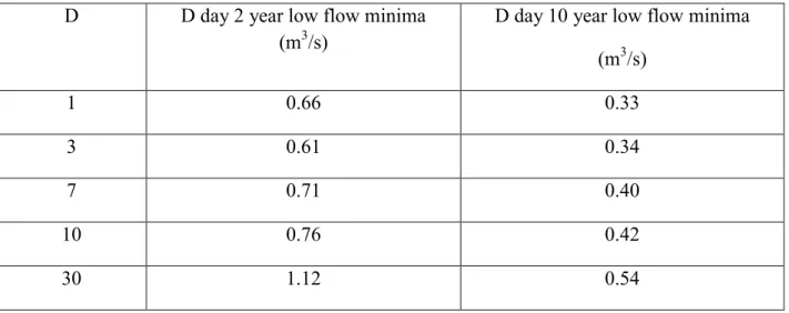
Figure 5 shows the LFFC for annual minima, 3, 7, 10 and 30 days flow minima. The data are plotted in semi-logarithmic axis. It can be seen that there is not much difference between D-day LFFC, where D=1, 3, 7, 10 days. However, these curves are markedly different from 30 days LFFC. Some countries base water quality standards on low flow conditions such as 7 day, 2-year low flow (McMahon and Mein, 1986) and 7-day, 10-year low flow (Characteristics of low flows, 1980). These indices are shown in Table 2.
Figure 5: Frequency-duration curves for the annual minima series, river Ouelle. Data are
14
Table 2: D day d year low flow minima where D=1, 3, 7, 10 and 30 days and d=2, 10 years D D day 2 year low flow minima
(m3/s)
D day 10 year low flow minima (m3/s) 1 0.66 0.33 3 0.61 0.34 7 0.71 0.40 10 0.76 0.42 30 1.12 0.54
LFFC are informative in several respects but they provide no information about the length of periods below a particular level (threshold) and the deficit (volume) of flow that is built up during a continuous low flow event. Streams with similar LFFC may have show low flow sequences. One may have few long intervals and the other may have many short intervals below the same flow level. A widely used approach to account for these limitations involves the use of “truncation” level or “threshold level” which has originated from the theory of runs (Yevjevich, 1967; Zelenhasic and Salvai, 1987). A run is defined as the number of days when discharge falls below a certain threshold level which is governed by the objective of study and the nature of flow regime considered. For example, the hydrological drought characterization of perennial rivers may be in the range of discharges with 70-90% exceedence on FDC (Smakhtin, 2001). To the end of the concept of „threshold level‟, this report discusses an application of Partial Duration Series (PDS) which analyses the frequency of low flows and flood peaks occurring below and above, respectively, a chosen threshold level.
15
6. Partial Duration Series
Flood frequency analysis is generally performed on a data series comprising of single highest peak in a year, known as the Annual Maximum Series (AMXS). For low flows, Annual Minimum Series (AMNS) is considered. Annual minimum series (AMNS) involves selecting single lowest value in each year. The value of low-flow frequency analysis can be improved by considering 7- day or 10- day moving averages of flow. AMNS in that case would involve annual minimum 7- day or 10- day flow. Flood frequency analysis is mainly centered on large infrequent floods because of their use in for the design of structures. Certain flows (for example, channel forming flows, flows that move the substrate) occur more than once in a year and annual maximum series do not account for these flows. An appropriate technique in such cases is the „Partial Duration Series‟ approach (PDS; Rosbjerg, 1985). PDS involves selecting those values that lie above (Peaks over threshold; POT) and below (Peaks below threshold; PBT) a threshold level, chosen for its relevance to the issue for which the analysis is being carried out. For this report, PBT are analyzed.
AMNS are analyzed differently from PBT. PBT involve more data than AMNS due to the inclusion of those low flow events that may not be the lowest flows in a year but are below a chosen threshold. Inclusion of more points in the analysis increases the possibility of flows below threshold being dependent on each other since the factors influencing one such value may influence others occurring within the same year or season too. For the example considered in this report, the threshold values were chosen so that the resulting series exhibit no interdependence. The threshold value of 1.10 m3/s was selected. The tests for independence, stationarity and
16
homogeneity of the resulting series were performed using HYFRAN. Both series were found to be homogenous, stationary and independent at 5% significance level.
From Figure 6, according to PDS (PBT) and AMNS, flows of magnitude 0.27 and 2.46 m3/s, respectively are occurring at average return Interval (ARI)=1 year. The lower quantile associated with PBT means that the minimum flow of 0.27 m3/s is not as rare as expected from AMNS. River Ouelle exhibits severe low flows in summers. Hypothetically, if the reservoir gets replenished in spring (snow-melt), then it may be able to release sufficient volume of water to sustain such a flow occurring in summer. But if this value reappears next year in winters, then there would be shortage of water for downstream users as the reservoir water levels would be low.
Figure 6: Partial duration series constructed for peaks below threshold (PBT). The threshold value selected is 1.10 m3/s
17
Record length is a crucial factor in frequency analysis studies. A large sample size is more likely to exhibit the features of the population of interest than a small sample size. Decreasing sample size introduces sampling errors and increases the inherent uncertainty related to the flow and recurrence interval relationship derived from the sampled data. Therefore, most of the frequency analysis methods rely on choosing distribution with the most appropriate shape for the data. Fitting distributions allow extrapolation of data beyond the range of observed values for a reliable estimation of flows.
7. Fitting distribution
The procedure includes trying to fit several theoretical distributions to the observed low flow data and selecting an appropriate distribution by using statistical tests. For low flows, the recommended distributions include Weibull, Gumbel, Pearson Type-III and lognormal distribution. Many studies have attempted to ascertain suitable distributions for annual minima and those occurring at different averaging intervals (Prakash, 1981; McMahon and Mein, 1986; Durrans, 1996). Despite several attempts, no fixed probability distribution for low flows has been agreed on. One of the crucial issues that most of LFFA and distribution fitting studies confront is the occurrence of zero values.
Hydrological datasets for example, streamflow and precipitation, often have zero as a lower limit. Ignoring zero values may lead to an unreliable estimation of the concerned variable. However, distributions fit to zero values assign positive probabilities to negative values of the variable. In such cases, the distributions can be restricted to have a lower limit, which may give physically meaningless results along with challenging the flexibility of the distribution (Smakhtin, 2001). In another approach, Hann (1977) used a conditional probability approach to
18
account for zero values of low flows. Using the theorem of total probability, for non-negative values of flows, denoted by x, this approach can be expressed as:
Proportion of values equating to zero are accounted for by primarily analyzing all non-zero observations and then multiplying the resulting probabilities by the fraction of non-zero values in the data. That is
Where is the probability of exceedence of all values, c is the probability that x is not zero and is the probability of exceedence for the non-zero values. Probability distributions are characterized by their parameters. To fit a distribution to a dataset, true parameter values of the same must be ascertained using the sample data series. Two dominant parameter estimation techniques exist:
Method of maximum likelihood Method of Moments
7.1 Method of maximum likelihood
Consider a sample of N random variables which are independent and identically distributed according to the probability density function , where
are parameters. The likelihood function is defined as
19
since are independent and identically distributed.
The objective is to maximize the likelihood function (L), i,e. to find the values of that make the data ( most probable. The maximum of the likelihood function is given by
Where j=1, 2,…,N
7.2 Method of Moments
The method of moments consists of equating sample moments with theoretical moments . For a sample of N observations ,
is the rth theoretical moment about origin and
is the rth theoretical moment about mean
is the rth sample moment about origin and
is the rth sample moment about sample mean
For this report, method of maximum likelihood is used for parameter estimation. Once the parameters are estimated, the selected distributions are tested for the hypothesis that the observed data are actually from the fitted probability distribution. Two commonly used methods are chi-square test (Huang et al., 2008) and Kolmogorov Smirnov test (McCuen, 2003). According to Hann (1977), the goodness of fit tests are discouraged when fitting distributions to streamflow data because of their insensitivity in the tails of the distribution. Also, these tests may give
20
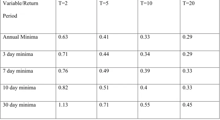
misleading results when the sample size is small; i.e., probability of accepting the hypothesis that the distribution fits, when in fact it does not, is high. But these tests help when comparing the relative merit of one distribution over another. Figure 7 shows Generalized extreme value distribution (GEV) fitted (best fit according to AIC and BIC criteria) to annual minima series of river Ouelle. Figure 8 shows the distributions fitted to the 3, 7, 10, 30 days. Lognormal distribution was found suitable for all moving average annual minima series according to the corresponding AIC and BIC values. The estimates of these variables obtained using the selected distributions are mentioned in Table 3.
Figure 7: Generalised Extreme Value distribution fitted to annual minima series, river Ouelle
21
Figure 8: Lognormal distribution fitted to 3, 7, 10 and 30 day moving average minima, river Ouelle.
Table 3: Estimates of annual minima and 3, 7, 10 and 30 day minima for return periods (T) = 2,5,10 and 20 Variable/Return Period T=2 T=5 T=10 T=20 Annual Minima 0.63 0.41 0.33 0.29 3 day minima 0.71 0.44 0.34 0.29 7 day minima 0.76 0.49 0.39 0.33 10 day minima 0.82 0.51 0.4 0.33 30 day minima 1.13 0.71 0.55 0.45
22
Figure 9 and 10 shows GEV and GP distribution fitted to PBT (using MATLAB) obtained for thresholds= 1.1 m3/s (104 points) and 0.7 (76 points). Both the series satisfied the conditions of stationarity, homogeneity and independence at 5% significance level. Estimates obtained using these distributions for both the cases are compared in Figure 11. In both cases GEV distribution better fitted the PBT series in comparison to GP. For the latter, the fit was better for threshold=1.1 m3/s. For a particular year, not all flow values below threshold can be selected to form PBT series as they may be dependent on each other. Therefore, different sets of low flow series can be obtained with flows below threshold and satisfying the conditions of independence, stationarity and homogeneity. Estimates from two such PBT series (both having 104 points) obtained using threshold=1.1 m3/s and GEV distribution fitted to each are compared in Figure 12. Marked differences were observed between the two considered series for higher return periods (10, 20 years).
Figure 9: Generalised Extreme Value and Generalised Pareto distribution fitted to Peaks below threshold (PBT) with threshold value=1.1m3/s (46 years of data; 104 values)
23
Figure 10:Generalised Extreme Value and Generalised Pareto distribution fitted to Peaks below threshold (PBT) with threshold value=0.7 m3/s (46 years of data; 76 values)
Figure 11: Comparison of return periods obtained using GEV and GP distributions for threshold values =1.1 m3/s and 0.7 m3/s
24
Figure 12: Comparison between the estimates given by GEV distribution for two sets of PBT obtained for threshold=1.1 m3/s
Several indices can be found in literature that view low flow regime of a river from different perspectives. Based on the work of Daigle et al. (2010), six such indices (Table 4) have been considered for river Ouelle. There are five yearly and one seasonal index (July-October). The selection of these indices was based on the following criteria:
1. Indices explain 75% of the variance of hydrological indices describing the low flow regime of rivers in Eastern Canada
25
Table 4: Indices describing low flows in river Ouelle from four aspects: Amplitude, variability, timing and duration
Index Description Timing
A1 Mean of the minimums of all March flow values over the entire record (Ls-1km-2)
Yearly A2 Ratio of the lowest annual monthly discharge to
the mean annual discharge (unitless) Yearly T1 Average Julian date of the seven annual 1-day
minimum discharges (Julian date) Yearly V Standard deviation of the Julian date of the
seven 1-day minimum discharges (days)
Yearly D1 90-day minimum divided by the median of the
entire record(unitless)
Yearly D2 90-day minimum calculated for July-October,
divided by the median of the entire record (unitless)
Seasonal
The present report attempted to fit distributions to these indices and the ones (A1, A2, T1 and V) calculated using 3, 7, 10 and 30 day moving averages of flow. Box plots comparing the indices calculated from moving averages is shown in Figure 13. For indices A1 and A2, there was no marked difference between the indices calculated from 3, 7 and 10 day moving averages. In the case of 30 day moving average, the median values of A1 and A2 show 6% and 12% increase. For index T1, 4, 15, 21 and 54% decrease in the median values was observed for this index calculated from 3,7,10 and 30 day moving averages, respectively. For river Ouelle, one day minima occur systematically in summer (July-October). Moving average filtering reduces the effects of random variations. Therefore, averaging adjacent measurements will eliminate the random fluctuations, with the result shifting the occurrence of one day minima to winters (December to March). For index V, not much difference was observed between the median
26
values of the index corresponding to 3, 7, 10 and 30 day moving averages. The chosen distributions and corresponding parameters are shown in Table 5. No distribution was found to fit index T1 and V for all moving averages. For indices A1, the distribution fitting the considered indices obtained from 30 day moving averages was Gamma whereas for the remaining it was Lognormal. For index A2, Gamma distribution was selected for all moving averages. For D1 and D2, Gamma and Lognormal distribution were found to best fit the data
Table 6 shows the comparison of the quantiles obtained from fitted distributions. Estimated values of the considered low flow indices (LF, LF_3day, LF_7day, LF_10day and LF_30day; shown in Table 6) occurring at a recurrence interval (T) = 2, 5, 10 and 20 and 100 years are shown. Since no distribution was found to fit index T1 and V, estimates for these indices are not shown. D1 and D2 are already duration indices and therefore estimates only for the indices are shown. For T=2, highest value of the corresponding estimate of index A1 is observed for LF_30days (1.68 m3/s) and lowest value for LF_10days (1.48 m3/s). For T=5, highest value of magnitude 0.872 m3/s was observed for LF_30days. For T=100, highest value of A1 was observed for LF_7days (0.312m3/s) and lowest value for LF_30days (0.229m3/s). For index A2, it is observed that for all return periods T=2, 5, 10, 20 and 100, the estimates have shown an increase from the 3 to 30 day moving average. For D1 and D2, estimates of LF have shown a decrease from T=2 to T=100. The estimates for T=2 are 0.306 and 0.508 for D1 and D2 respectively. For T=100, the estimates for D1 and D2 are 0.0724 and 0.102.
27
Figure 13: Box plots showing the low flow indices and the ones calculated using 7, 10 and 30 day moving averages for A1, A2, T1 and V
Table 5: Distributions chosen for the selected indices using HYFRAN/MATLAB Index/Dura
tion
Original values of the index
3 Days 7 Days 10 Days 30 Days A1 Lognormal Mu: 0.44 Sigma: 0.70 Lognormal Mu:0.44 Sigma: 0.70 Lognormal Mu: 0.44 Sigma: 0.69 Lognormal Mu:0.39 Sigma:0.70 Gamma Mu:1.072 Sigma:2.39 A2 Gamma Mu:33.43 Sigma:3.85 Gamma Alpha:35.87 Lambda:4.07 Gamma Alpha:34.96 Lambda:4.09 Gamma Alpha:34.22 Lambda:4.12 Gamma Alpha:37.59 Lambda:4.92 T No distribution No distribution No distribution No distribution No distribution
28
found found found found found
V No distribution found No distribution found No distribution found No distribution found No distribution found D1 Gamma Alpha:12.73 Lambda:4.22 - - - - D2 Lognormal Mu:-0.67 Sigma:0.78 - - - -
Table 6: Estimates of fitted distribution shown in Table 5 Return
period
Low flow Index(LF)
LF_3days LF_7days LF_10days LF_30days
A1 (m3/s) T=2: T=5: T=10 T=20 T=100: 1.55 0.858 0.629 0.487 0.302 1.54 0.854 0.626 0.485 0.300 1.54 0.866 0.640 0.499 0.312 1.48 0.821 0.604 0.469 0.292 1.68 0.872 0.585 0.407 0.183 A2
29 T=2: T=5: T=10 T=20 T=100: 0.105 0.0652 0.0492 0.0383 0.0228 0.104 0.0657 0.0501 0.0394 0.0240 0.108 0.0677 0.0517 0.0407 0.0248 0.111 0.0698 0.0533 0.0420 0.0315 0.122 0.0804 0.0632 0.0511 0.0331 D1 T=2: T=5: T=10 T=20 T=100: 0.306 0.194 0.149 0.118 0.0724 - - - - D2 T=2: T=5: T=10 T=20 T=100: 0.508 0.263 0.186 0.140 0.102 - - - -
30
8. Conclusion
Flow duration curves are the graphical means of expressing the relationship between magnitude and frequency of streamflow discharges. These curves can be constructed for different time periods: annual, month, seasonal and daily. Various indices characterising low flows can be obtained from FDCs (Flows with 70-99% exceedence, Q20/Q90, Q50/Q90 and Q90/Q50). Another graphical means of understanding the characteristics of low flows is Low flow frequency curves (LFFC). Like FDCs, LFFC can also be used to obtain several indices (7 day 10 year flow, 7 day 2 year flow etc.) that describe low flow regime of a river. Although these curves are informative in many respects, they provide no information about the duration and intensity of low flow events. To this end, the concept of partial duration series emerged as a means of accounting for these limitations.
PDS involves analyzing flow events below (PBT) or above (Peaks Over Threshold; POT) a chosen „threshold level‟. The choice of threshold relies on the nature of objectives in hand. PDS are preferred over annual minimum series for studies requiring information about flows occurring more than once in a year (e.g. channel forming flows). The results obtained from PBT analysis relies on the chosen threshold level and the selected flow values below this threshold. Although these frequency analysis methods are informative in understanding low flows, their performance is influenced by sample size. Due to the limitations imposed by sample size, different types of theoretical distribution functions are fitted to the concerned variables to give better estimates and allow extrapolation beyond the limits of „observed‟ probabilities.
Generalised extreme value distribution was found to fit annual minima series. For 3,7,10 and 30 day moving average annual minima, lognormal distribution was selected as the best fit. For the
31
PBT series, a threshold value of 1.1 m3/s was used. Using this series, 104 points were selected, below this threshold and satisfying the conditions of independence, stationarity and homogeneity. PBT series was found suitable over annual minima for flows with recurrence interval less than four years. GEV and GP were fitted to PBT series and GEV (AIC=-88.175) was found a better fit than GP (AIC=-71.4433). The effect of threshold on the estimates given by fitted distributions was experimented by forming the PBT series using threshold =0.7 m3/s. GEV (AIC=-164.52) better fitted the resulting series than GP (AIC= -133.3729). Estimates for T= 2 and 5 years were close to each other but noticeable differences were observed for T=10 and 20 years. Six indices describing the low flow regime of river Ouelle were also selected for fitting distributions. These indices described four aspects of low flow regime: magnitude, timing, variability and duration. These indices were also calculated for 3,7,10 and 30 day moving averages. Lognormal distribution was found to fit index A1, for 3, 7 and 10 day moving average whereas for 30 day moving average, gamma distribution was regarded a better fit. For index A2, Gamma distribution was selected for all moving averages. No distributions were found for indices T1 and V. For D1 and D2, Gamma and Lognormal distributions were selected as best fit.
32
9. References
.
Bovee, K.D. 1982. A guide to stream habitat analysis using the Instream Flow Incremental Methodology. Instream Flow Information Paper 12. United States Fish and Wildlife Service FWS/OBS- 82/26. 248pp.
Characteristics of low flows, 1980. J. Hydraul. Div. ASCE, 106 (HY5), 717–737.
Cunnane, C., 1978. Unbiased plotting positions-a review. Journal of Hydrology, 37, 205-222. Dairymple, T., 1960. Flood frequency analysis. US Geol. Surv. Wat. Supply Pap. 1543-A
Durrans, S.R., 1996. Low-flow analysis with a conditional Weibull tail model. Water Resour. Res. 32 (6), 1749–1760.
Haan, C.T., 1977. Statistical Methods in Hydrology. Iowa State University Press, Ames, IA. Hosking, J.H.M., Wallis, J.S. & Wood, E.F.(1985)Estimation of the generalized extreme value distribution by the method of probability weighted moments. Technometrics, 27(3), 251-261 Huang et al., 2008
Kroll, C.N. and Vogel, R.M., 2002. Probability distribution of low streamflow series in the United States. Journal of Hydrologic Engineering, Vol. 7, No. 2,137-146
Lall,U., 1995. Recent advances in non-parametric function estimation: hydrological applications. Rev. Geophys. (Suppl.), 1093–1102.
Matalas, N.C., 1963. Probability distribution of low flows. USGS Professional Paper 434-A, USGS, Washington, DC
33
McMahon, T. A. & Mein, R.G. (1986) River and Reservoir Yield. Water Resources Publications, Liuleton, Colorado
Ouarda, T.B.M.J., Christian C. and St-Hilaire, A., 2008. Statistical models and the estimation of low flows. Vol 33(2) 195-206.
Huang, Y-P, Lee, C.H., Ting, C.S., 2008. Improved estimation of hydrologic data using the Chi-Square goodness-of-fit test.Vol. 31, No. 3, pp. 515-521
Prakash, A., 1981. Statistical determination of design low flows. J. Hydrol. 51, 109–118. Smakhtin, V. U., 2001. Low Flow Hydrology-A review. Journal of Hydrology 240, 147-136 Rosbjerj, D. 1985. Estimation in partial duration series with independent and dependent peak values. Journal of Hydrology, Vol 76,183-195
Tasker, G. D., 1980. Hydrologic regression with weighted least squares. Water Resour. Res. 16 (6), 1107–1113
Vogel, R.M., Kroll, C.N., 1989. Low-flow frequency analysis using probability-plot correlation coefficients. J. Water Res. Plan. Manag. (ASCE) 115 (3), 338–357.
Yevjevich, V., 1967. An objective approach to definitions and investigations of continental hydrologic droughts. Colorado State University, Fort Collins, Hydrology Paper 23, 18 pp. Zelenhasic, E., Salvai, A., 1987. A method of streamflow drought analysis. Water Resour. Res. 23 (1), 156–168.