Dynamique moléculaire non-adiabatique des complexes de type PAH

(1)

THÈSE

En vue de l’obtention du

DOCTORAT DE L’UNIVERSITÉ DE TOULOUSE

Délivré par l'Université Toulouse 3 - Paul Sabatier

Présentée et soutenue par

Evgeny POSENITSKIY

Le 29 septembre 2020

Dynamique moléculaire non-adiabatique des complexes de type

PAH

Ecole doctorale : SDM - SCIENCES DE LA MATIERE - Toulouse

Spécialité : Physique

Unité de recherche :

LCAR-IRSAMC - Laboratoire Collisions Agrégats Réactivité

Thèse dirigée par

Didier LEMOINE et Fernand SPIEGELMAN

Jury

Mme Valérie VALLET, Rapporteure M. Rodolphe VUILLEUMIER, Rapporteur

M. Thomas NIEHAUS, Examinateur Mme Christine JOBLIN, Examinatrice M. Didier LEMOINE, Directeur de thèse M. Fernand SPIEGELMAN, Co-directeur de thèse

(2)

(3)

Non-adiabatic

molecular dynamics

of

PAH-related complexes

Evgeny Posenitskiy

Toulouse, France Submitted: August 2020 Defended: September 2020

(4)

(5)

Abstract

Polycyclic Aromatic Hydrocarbons (PAHs) have been proposed as main carriers of diffuse interstellar bands that are observed in the interstellar medium. This has motivated an extensive study of their photophysical and photochemical response to UV irradiation. Underlying competing mechanisms drive the evolution of gas in the interstellar medium. The main objective of this thesis is to describe and to get theoretical insight in the energy relaxation mechanisms in large PAH molecules via extensive non-adiabatic molecular dynamics simulations coupled to the linear response Time-Dependent Density Functional based Tight Binding (TD-DFTB) approach of the excited states.

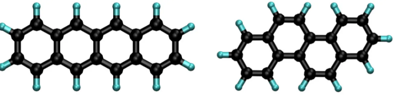
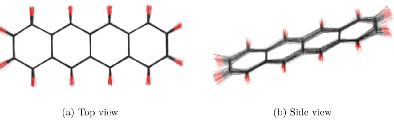
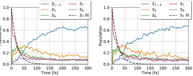
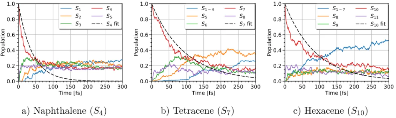
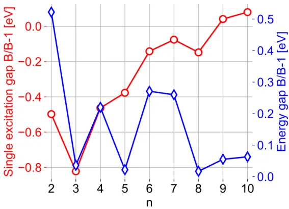
Prerequisite substantial development was made in the DFTB deMon-Nano package (http:// demon-nano.ups-tlse.fr), firstly with the implementation of analytical gradients of potential energy surfaces (PESs) and of non-adiabatic couplings within the TD-DFTB scheme. Next, the Tully’s fewest-switches trajectory surface hopping (FSSH) algorithm has been adapted and coupled to the TD-DFTB scheme in order to take into account non-adiabatic transitions. After detailed methodological considerations and comparison with higher-level electronic structure methods, the first full-scale application is dedicated to non-adiabatic molecular dynamics of linearly cata-condensed PAHs. Electronic relaxation from the brightest excited state has been simulated for neutral polyacenes with 2 to 7 aromatic cycles. The results display a striking alternation in decay times of the brightest singlet state computed for polyacenes with up to 6 aromatic cycles, which is correlated with a qualitatively similar alternation of energy gaps between the brightest state and the state lying just below in energy. Next, the influence of geometry on relaxation has been investigated through the comparison of two isomers: armchair-edge chrysene versus zigzag-armchair-edge tetracene. After assessing the performance of DFTB parameter sets, the main focus is given to the analysis of the electronic relaxation from the brightest excited state, which is located around 270 nm for both isomers. The results show that the electronic population of the brightest excited state in chrysene decays an order-of-magnitude faster than that in tetracene. This is correlated with a significant difference in energy gaps between the brightest state and the state lying just below in energy, which is consistent with the previous conclusions for polyacenes.

A last major development concerns the use of Machine Learning (ML) algorithms that have been proposed as a way to avoid most of the computationally-demanding electronic structure calculations. It aims to assess the performance of neural networks algorithms applied to excited-state dynamics. Electronic relaxation in neutral phenanthrene has been chosen as a

(6)

iv 0 Abstract

test case due to the diversity of available experimental results. Several neural networks have been trained with different parameters and their respective accuracy and efficiency analyzed. In addition, approximate trajectory surface hopping schemes have been interfaced to ML-based PESs and gradients, resulting in non-adiabatic dynamics simulations at a negligible cost. Various simplified hopping approaches have been compared with FSSH. Overall, ML is found to be a highly promising tool for nanosecond-long molecular dynamics in excited states. This PhD research opens new avenues to investigate theoretical photophysics of large molecular complexes. Last but not least, the theoretical tools developed and implemented in deMon-Nano in a modular way can be further combined with other advanced (such as Configuration Interaction) DFTB techniques better adapted to charge-transfer states.

(7)

Résumé

Les hydrocarbures aromatiques polycycliques (PAH) ont été proposés comme porteurs prin-cipaux de bandes interstellaires diffuses observées dans le milieu interstellaire, motivant des études approfondies de leur réponse photophysique et photochimique au rayonnement UV. Les mécanismes sous-jacents en compétition déterminent l’évolution du gaz dans le milieu interstellaire. L’objectif principal de cette thèse est de décrire et de comprendre les mécanismes de relaxation dans des PAHs de grande taille, par des simulations de dynamique moléculaire non-adiabatique, couplées à l’approche de la réponse linéaire ”Time-Dependent Density Functional based Tight Binding” (TD-DFTB) des états excités.

Des développements substantiels, prérequis ont été effectués dans le code DFTB deMon-Nano (http://demon-nano.ups-tlse.fr), d’abord avec le calcul des gradients analytiques des surfaces d’énergie potentielle (PES) et des couplages non-adiabatiques des états TD-DFTB. Puis, l’algorithme de trajectoire à sauts de surface minimaux (FSSH) de Tully a été adapté à l’approche TD-DFTB afin de prendre en compte les effets non-adiabatiques. Après comparaison avec des méthodes de structure électronique de référence, la première application est dédiée à la dynamique non-adiabatique de PAHs cata-condensés linéairement. La relaxation électronique de l’état excité le plus brillant a été simulée pour des polyacènes neutres constitués de 2 à 7 cycles aromatiques. Les résultats montrent une alternance marquée dans les temps de dépopulation de l’état initial pour les polyacènes contenant jusqu’à 6 cycles aromatiques, ce qui est corrélé avec une alternance des écarts d’énergie entre l’état initial et l’état situé juste dessous. Puis, l’influence de la géométrie sur la relaxation a été étudiée en comparant deux isomères, le chrysène de type ”armchair-edge” et le tétracène de type ”zigzag-edge”. Après évaluation des paramétrages DFTB, la relaxation électronique à partir de l’état excité le plus brillant, situé autour de 270 nm pour les deux isomères, à été analysée. Les résultats montrent que la population électronique excitée du chrysène décroît un ordre de grandeur plus rapidement que celle du tétracène. Ceci est aussi corrélé à une différence significative des écarts d’énergie entre l’état initial et l’état situé juste dessous.

Un dernier développement majeur concerne l’utilisation d’algorithmes ”Machine Learning” (ML) proposés comme un moyen d’éviter la plupart des calculs de structure électronique, très coûteux en temps calcul. Les performances d’algorithmes de réseaux de neurones appliqués à la dynamique des états excités ont été évaluées. Le cas de la relaxation électronique dans le phénanthrène neutre a été choisi comme test en raison de divers résultats expérimentaux disponibles. L’apprentissage de plusieurs réseaux de neurones a été effectué et leurs précision

(8)

vi 0 Résumé

et efficacité analysés. De plus, des approximations de trajectoires à sauts de surface ont été interfacées à l’approche ML, résultant en un coût négligeable des simulations de dynamique non-adiabatique. L’efficacité des diverses approches simplifiées a été comparée à FSSH. Dans l’ensemble, ML se révèle un outil très prometteur pour la dynamique dans les états excités à l’échelle de la nanoseconde.

Ce travail de thèse ouvre de nouvelles voies pour étudier la photophysique théorique de complexes moléculaires de grande taille. Enfin, les outils développés et implémentés dans deMon-Nano, de manière modulaire, peuvent être combinés avec d’autres approches DFTB sophistiquées (tel que ”Configuration Interaction”) plus adaptées aux états à transfert de charge.

(9)

1 Introduction

One of the main objectives in astrophysics is to understand and describe the evolution of the universe and galaxies within. Modern models assume that this evolution is mostly governed by balance between the formation and destruction of stars within each galaxy.[1]

Stars are formed from collapsing clouds of condensed gas and dust, the so-called molecular clouds, and evolve differently depending on their mass. For instance, the existence of a massive star ends with an explosion called supernova. This is followed by release of the heavy elements that had been formed inside the star. Evolution of stars that are not that massive is governed by the stellar winds that drag away molecules and dust from the circumstellar environments into the Interstellar Medium (ISM). The matter travels in the ISM and is gathered into denser clouds, namely the molecular clouds. Once a critical mass is accumulated, the molecular cloud may collapse and form stars. This couples the life cycle of the stars to the evolution of gas and dust, thus forming a closed loop that is schematically represented in Figure 1.1.

The ISM of our galaxy consists of two parts: gas (about 90% hydrogen, 10% helium and a small fraction of carbon, oxygen, nitrogen and some other elements) and dust nanoparticles (mostly silicates and carbon). In dense molecular clouds, the gas temperature varies from ∼1000 K in the external layers illuminated by UV photons to ∼10 K in the inner regions. This change in temperature is mostly governed by the penetration depth of the stellar UV radiation. These photodissication regions[2]_{(also called photon-dominated regions or PDRs) associated with star}

forming areas gained a lot of attention in recent years. In the cold inner regions, the H2 and

CO survive and can be used to track the evolution of molecular gas. On the contrary, UV radiation may dissociate these molecules and ionize released fragments (for example, forming C+_{) in the warmer regions. All the aforementioned regions represent a unique playground for}

astrochemistry and astrophysics research that aims to understand the evolution of the ISM but also to study molecular processes.

(12)

2 1 Introduction

Figure 1.1: Sketch of the various stages in the life cycle of stars and matter in the galaxy. Reproduced from Kulesa et al. (2012). Opportunities for Terahertz Facilities on the High Plateau. Proceedings of the International Astronomical Union, 8(S288), 256-263 with permission from Cambridge University Press.

1.1 A few words about photophysics

One way to trace the evolution of remote objects (e.g. interstellar regions) is via spectroscopical analysis. Owing to the technological advancements in various fields, many telescopes have been built and numerous observations have been performed in recent years. In particular, Herschel and Spitzer missions provided spectral and spatial information about the infrared (IR) emission for many astrophysical environments in several galaxies.[3]

Some basic photophysical concepts have to be introduced in order to better understand the evolution of molecular complexes following absorption of photons. Figure 1.2 shows several types of relaxation upon absorption of an ultraviolet (UV) light by an isolated molecule. The case of dissociation/fragmentation has not been considered here even though it is responsible for a significant amount of the interstellar chemistry. In fact, there are many chemical reactions that play a crucial role in the evolution of the ISM (see Table1.1). It is also worth mentioning photoisomerization as one of the most important photochemical processes.[5]

(13)

1.1 A few words about photophysics 3

Figure 1.2: Possible decay pathways for a photoinduced process according to Ref. [4] . Table 1.1: Important chemical reactions in the ISM.

Bond formation

Radiative association A + B → AB + hν

Grain surface formation A + B : g → AB + g Associative detachment A− _{+ B → AB + e}− Bond breaking Photodissociation AB + hν → A + B Dissociative recombination AB+ _{+ e}− _{→ A + B} Collisional dissociation AB + M → X + Y + M Rearrangement reactions Ion-molecule exchange A+ _{+ BC → AB}+ _{+ C} Charge transfer A+ _{+ B → A + B}+ Neutral collisions A + BC → AB +C

Consider now a molecular system in its ground (equilibrium) state. Once a photon is absorbed, the system gains an excess of energy that promotes it to an excited state. The subsequent relaxation can be roughly divided in two branches depending whether there is a photon emission or not:

(14)

4 1 Introduction

• The system may reach a certain excited state after a cascade of radiationless transitions and emit a photon from this state. This emitted photon will carry an excess of energy, thus bringing the system back to the ground state. Fluorescence (phosphorescence) corresponds to an emission from an excited singlet (triplet) state. This is a radiative process;

• Alternatively, a cascade of transitions may bring the system all the way back to the ground state. Thus, an excess of energy is translated into the heat. Since no emission is involved, this process is non-radiative.

The Jablonski diagram (see Figure 1.3) is commonly used to represent the complexity of photophysical processes. It takes into account the vibrational relaxation (radiative transitions between vibrational modes), which is responsible for the IR emission. The number of vibrational degrees of freedom is 3N–6 for a molecule with N atoms. It is worth mentioning that the vibrational relaxation in an isolated system is driven by the coupling between the initally excited and the remaining vibrational modes. Thus, the IR spectroscopy is a powerful tool that can be used to distinguish the chemical families of complex molecular systems. While the IR emission can be observed in the ground state, the fluorescence (phosphorescence) is related to excited states only. The timescales of the latter processes are significantly (by several orders of magnitude) lower than in case of an internal conversion or vibrational relaxation. If the emitted photon carries energy in the range of 380 to 750 nm, then such light falls in the visible part of the spectrum (often called UV-vis or visible UV).

Figure 1.3: Simplified Jablonski diagram representing different relaxation pathways following

absorption of a UV photon. Intersystem crossing (ISC) is a radiationless transition between singlet and triplet states.

(15)

1.2 The PAH hypothesis 5

1.2 The PAH hypothesis

The analysis of the dust emission in astrophysical objects has indicated the presence of some characteristic features in the mid-infrared (around 3.3, 6.2, 7.7, 8.6 and 11.3 µm). These bands are now known as Aromatic Infrared Bands (AIBs). More bands are observed with a higher resolution in several astronomical objects (see Figure 1.4).

Figure 1.4: The ISO-SWS spectra of the nucleus of the galaxy NGC 4536, planetary nebula

NGC 7027 and the photo-dissociation region at the Orion bar. Aromatic modes of the major PAH vibrations are indicated on the top axis. Reproduced from Els Peeters (2011). The PAH Hypothesis after 25 Years. Proceedings of the International Astronomical Union, 7(S280), 149-161 with permission from Cambridge University Press.

AIBs were initially attributed to very small grains.[6] _{Later on, Léger and Puget}[7] _and

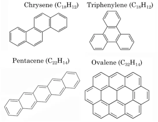
Allamandola et al.[8] _{proposed that Polycyclic Aromatic Hydrocarbons (PAHs, see Figure} _1.5)

are the carriers of these bands. PAHs are organic molecules that are composed of two or more carbonaceous hexagons (aromatic carbon rings) with peripheral hydrogens. These rings result

(16)

6 1 Introduction

from the sp2 _{bonds between carbon atoms and grant the aromaticity to the corresponding}

molecule. Some PAHs can be called peri-condensed if there are carbon atoms that are shared between three rings and cata-condensed if carbon atoms are located in one or maximum two successive rings. The PAH hypothesis is based on the assumption that PAH molecules reach high temperatures following the absorption of a UV photon and then radiatively cool down via an IR emission. They can survive the UV radiation due to their remarkable stability. Notably, some AIBs have been attributed to aliphatic (methylated) groups by Joblin et al.[9]_{More details}

about the PAH hypothesis can be found in Refs. [10,11] and references therein.

Figure 1.5: Several PAH molecules. Left and right columns correspond to cata- and

peri-condensed morphologies, respectively.

The aforementioned PAH model suffers from the lack of identification of individual species. However, PAHs also have absorption bands in the visible and UV range. In fact, Diffuse Interstellar Bands (DIBs), that fall essentially in the visible range,[12] _{might be due to ionized}

PAH compounds[13–17] _{and these bands may hold important clue for the identification of}

individual interstellar PAHs. This motivated many experimental and theoretical investigations of static[13,18–21] _{and dynamical}[22–26] _{properties of charged PAHs. However, less information}

about the photophysics of large neutral PAH molecules is available, despite the fact that they cannot be excluded from contributing to the DIBs.[14]

Up to date, not a single PAH has been unambiguously assigned as a DIB carrier. Furthermore, Peeters et al.[27] _{have noticed that the shape of AIBs does not vary significantly in different}

(17)

1.3 Theoretical considerations 7 number of large and compact PAHs (the so-called ”grandPAH” hypothesis)[28]_{or from a random}

mixture of many different compounds[29]_{. On the other hand, the role of derivative species like}

nitrogenated PAHs (nitro-PAHs), PAH clusters and PAH complexes with metals is yet to be precised.

It is worth mentioning two laboratory studies that have confirmed C+

60[30], C60and C70[31]as the

carriers of DIBs. Recent work by Palotás et al.[32] _{on protonated buckminsterfullerene C} 60H+

has indicated its possible contribution to the IR emission in the regions with high abundances of C₆₀. Another recent theoretical study has addressed the dual photophysical behaviour of C+

60

upon near-IR and UV excitations.[33]

1.2.1 Laboratory spectroscopy of PAHs

It is hard to imagine further development and assesment of the PAH hypothesis without the support from laboratory research. This has motivated many spectroscopical studies on PAH compounds both at the experimental and theoretical levels (see Ref. [11] and references therein). Numerous infrared and ultraviolet spectra have been measured or calculated for neutral and charged species of different sizes. These results have been compiled in spectroscopic atlases like Refs. [34,35] and free online databases developed by Malloci et al.[36]_{and Bauschlicher et al.}[37]

(hosted by OAC-Cagliari1 _{and NASA AMES}2_{, respectively).}

PAHs may also provide a catalytic surface for H2 formation in the ISM.[38] The group of

Prof. Liv Hornekær from Aarhus University has studied the hydrogenation patterns of neutral PAHs with the help of scanning tunneling microscopy, mass spectroscopy and theoretical cal-culations. The superhydrogenated coronene (C24H36)[39] and pentacene (C22H36)[40]have been

demonstrated to act as possible catalysts for molecular hydrogen formation under interstellar conditions. Work on hydrogenated buckminsterfullerene C₆₀is currently in progress.

The EUROPAH Marie Skłodowska-Curie project3 _{aims to understand the role that PAHs play}

in the physics and chemistry of the ISM. The present PhD thesis is part of this collaborative effort that brings together 16 PhD students from 9 universities.

1.3 Theoretical considerations

Quantum Chemistry and Materials Science are rapidly developing fields. Many useful molecular or solid state properties can be derived from a solution of the time-independent Schrödinger equation. However, solving this equation for many-body systems is a challenging and com-putationally demanding problem. One breakthrough in the field was the development of the

1_{http://astrochemistry.oa-cagliari.inaf.it/database/pahs.html} 2_{http://www.astrochem.org/pahdb}

(18)

8 1 Introduction

Hartree-Fock (HF) approach in the late 1920s. The main idea behind it is that the exact N-body wavefunction of the system can be approximated by a single Slater determinant. By invoking the variational method, one can derive a set of N coupled equations for N spin orbitals. A self-consistent solution of these equations yields the HF wavefunction and energy of the system. The original HF approach as well as the so-called post-HF wavefunction methods are often limited to small systems. Later on, Hohenberg and Kohn[41] _{proved that the ground state electronic}

energy is determined completely by the electron density. This theorem lies in the foundation of what is called Density Functional Theory (DFT) nowadays. Even though a different density in principle yields to a different ground state energy, the functional that maps one to another remains unknown. For more details, see Chapter2.

Understanding the photophysics of PAHs is a crucial and challenging problem for modern Quantum Chemistry. Naphthalene (the smallest PAH) has 10 carbon and 8 hydrogen atoms or 48 valence electrons. Taking into account that calculation of some integrals in Quantum Chemistry has the O(n4_{) complexity, where n is the number of electrons (actually up to}

O(n8_{) for wavefunction-based methods}[42]_{), performing theoretical simulations on PAHs can}

be cumbersome if not unfeasible. Nevertheless, studies have been done both at the post-HF[43]

and DFT[44,45]_{levels of theory.}

Moreover, the MAD group from Université Toulouse III - Paul Sabatier and CNRS has addressed a broad range of theoretical challenges on PAH-related compounds. I would like to highlight some of them, in particular (i) anharmonic infrared spectroscopy of cationic [SiPAH] and [FePAH][46,47]_{, (ii) statistical dissociation/fragmentation}[48–53]_{and (iii) isomerization pathways}

and barriers[54]_{. More recently, Dubosq et al.}[55,56]_{have studied four structural families of C} 60

carbon clusters that might contribute to the AIBs[55] _{and the DIBs in the UV}[56] _{range of}

spectra. On the other hand, structural[57]_{, thermal}[58] _{and ionization}[59] _{properties of pyrene}

clusters have been investigated in great details.

The majority of the aforementioned studies has been performed with a Density Functional based Tight-Binding (DFTB) method that is a simplified and computationally efficient (compared to the conventional DFT) approach for electronic structure calculations. The DFTB, combined with molecular dynamics, allows for an exhaustive exploration of Potential Energy Surfaces (PESs) for relatively large compounds. Despite its success to describe the static and dynamical properties of some PAHs in the ground state, information about excited-state dynamics is generally missing. This is not an issue when one considers relatively slow (~ns or ~µs) processes. However, ultrafast (~as or ~fs) phenomena have gained a lot of attention in recent years.[22,23,25,26] _{Accurate description of the underlying quantum effects requires access}

to molecular dynamics beyond the Born-Oppenheimer approximation. Implementation and application of such non-adiabatic molecular dynamics coupled to the DFTB formalism is the main topic of the present PhD thesis.

(19)

1.3 Theoretical considerations 9

1.3.1 Non-adiabatic effects (or a few more words about photophysics)

Modelling the evolution of an extended molecular system following the absorption of a UV photon is a challenging task, which requires a fine description of the energy spreading over many electronic and nuclear degrees of freedom. Understanding the involved processes is however of primary interest to characterize the photostability or photochemistry as well as the competition between radiative and non-radiative relaxation channels.[5]

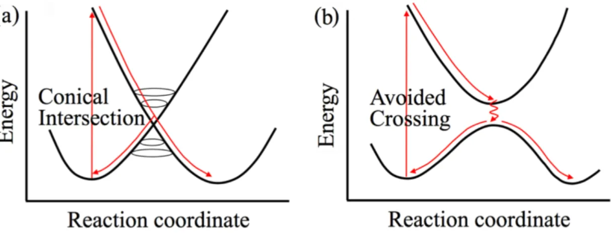
Figure 1.6: Schematic potential energy profiles for relaxation pathways through (a) a conical

intersection and (b) an avoided crossing. Adapted from the HDR thesis of Dr. Martial Boggio-Pasqua.[60]

Standard molecular dynamics usually relies on the Born-Oppenheimer approximation, which retains a single adiabatic electronic state in the expansion of a wavefunction of the system. This approach works fine as long as nuclei are considered as slowly moving particles (due to their higher mass compared to electrons). In the Born-Oppenheimer approximation, the nuclear dynamics obeys classical Newton’s equations of motion, while electrons are propagated using the time-dependent Schrödinger equation. However, in the regions where two or more electronic PESs are getting close (e.g. in the vicinity of a conical intersection, see Figure1.6), the nuclear and electronic degrees of freedom evolve with similar timescales and cannot be treated separately. This breakdown of the Born-Oppenheimer approximation requires to incorporate the non-adiabatic effects in order to render reliable quantum dynamics. Many approaches have been developed in recent years both at the ab initio[61]_{and mixed quantum-classical}[62–64]

levels of theory. One consists in propagating the time-dependent wavepacket as done in the Multi Configuration Time-Dependent Hartree (MCTDH) scheme.[65–67] _{This approach, which}

makes use of the ab initio PES fitted on a grid, usually allows to take into account only few electronic states and vibrational degrees of freedom due to the computational complexity of the propagation. Alternative schemes have been developed, relying on a classical description of nuclei, the two most popular ones being the mean-field propagation[68] _{and the Trajectory}

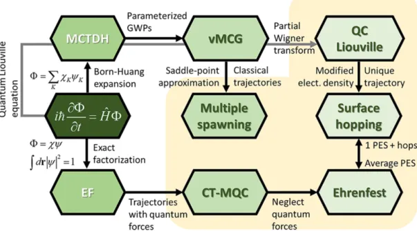
Surface Hopping (TSH). Schematic relation between different approaches to non-adiabatic dynamics is depicted in Figure 1.7. Starting from the exact time-dependent Schrödinger

(20)

10 1 Introduction

equation, the full molecular problem can be solved via (i) a Born-Huang expansion (as done in the MCTDH), (ii) an exact factorization of the molecular wavefunction or (iii) propagation of the density via Liouville equations. In the Born-Huang branch, the MCTDH combined with frozen Gaussian wavepackets approach renders the vMCG approximation, which, under certain conditions, converges to the Multiple Spawning.[69] _{In the exact factorization branch,}

a trajectory approximation of the nuclear wavepacket leads to a coupled-trajectory mixed quantum-classical method[70]_{, in which trajectories are coupled by quantum forces. If these}

quantum forces are neglected, the method reduces to the mean-field Ehrenfest approach.[71]

From the quantum-classical Liouville equations, assuming unique trajectories, large nuclear velocities and modifying the electronic density matrix, one can derive the fewest-switches trajectory surface hopping scheme.[72]_{For more details, see Ref. [73] and references therein.}

Figure 1.7: Schematic relation between different approaches to non-adiabatic molecular

dynamics. EF stands for Exact Factorization, GWP for Gaussian WavePacket and CT-MQC for Coupled-Trajectory Mixed Quantum-Classical approach. Adapted with permission from Rachel Crespo-Otero and Mario Barbatti (2018). Recent Advances and Perspectives on Nonadiabatic Mixed Quantum-Classical Dynamics. Chemical Reviews 118(15), 7026-7068). Copyright (2020) American Chemical Society.

The TSH approach is based on the idea that nuclei evolve on a given PES with a probability to switch states in the regions of strong non-adiabatic coupling. Historically, a Landau-Zener approach[74,75] _{has been developed for diabatic states’ crossing. Later on, Belyaev and}

Lebedev[76]_{adapted the Landau-Zener hopping probability for adiabatic states, which is better}

suited for practical applications due to the fact that Quantum Chemistry codes usually provide adiabatic energies and gradients. Alternatively, Zhu and Nakamura[77,78] _{have developed an}

(21)

1.3 Theoretical considerations 11 the Zhu-Nakamura theory, has gained a lot of attention in recent years partially due to its algorithmic simplicity and an absence of non-adiabatic coupling calculations. Yu et al.[79]

have developed a multidimensional extension of the Zhu-Nakamura theory and applied it to study the cis-trans isomerization of azobenzene. Their scheme has been further improved by Hanasaki et al.[80] _{and validated based on several analytical and ab initio models. Both studies}

indicate reasonable agreement with other theoretical approaches and available experimental data, especially taking into account an absence of non-adiabatic coupling terms. More recently, the Zhu-Nakamura theory has been combined with Machine Learning techniques,[81,82]

thus opening a promising direction for development and application of a long-scale quantum dynamics. Yet, one of the most commonly used TSH approaches is the Tully’s fewest-switches scheme.[83,84]_{It incorporates the electronic population and non-adiabatic coupling terms in the}

hopping probability, thus rendering a more accurate description of the electron dynamics. More details can be found in Section2.3of this thesis and Refs. [62,64,73] . It is worth mentioning that the calculation of non-adiabatic couplings consumes a significant amount of computational time even within the Time-Dependent Density Functional Theory (TD-DFT)[85]_{approach. The}

DFTB method has been extended by Niehaus et al.[86]_{to access electronic excited states leading}

to the TD-DFTB approach. It has been later on coupled to the nuclear dynamics via trajectory surface hopping schemes to study the non-adiabatic relaxation of large molecular systems.[87–90]

1.3.2 Bridging dynamical simulations and spectroscopic observations

Several studies at Imperial College London have been dedicated to the photophysics of cationic naphthalene[18]_{, pyrene}[19] _{and perylene}[20]_{. The presence of easily accessible sloped conical}

intersections suggests that naphthalene and pyrene radical cations are highly photostable, with an ultrafast non-radiative decay back to the initial ground state geometry. These studies are based on accurate but computationally demanding electronic structure methods like CASSCF and CASPT2. Notably, no accessible conical intersection with the ground state has been found in cationic perylene, which is consistent with experimental[91]_{observations.}

More recently, owing to the rapid development of High-Performance Computing centers, the research community has gained an access to large computational resources that allowed for an exhaustive exploration of PESs. While this is certainly possible with conventional static-like approaches, dynamical simulations represent a good alternative. Thus, excited-state dynamics comes into play to make its contribution in the field of spectroscopy. In particular, it is worth mentioning several theoretical works by the group of Prof. Susanta Mahapatra from University of Hyderabad. In 2010, Reddy et al.[22] _{have performed the MCTDH propagation of the six}

low-lying electronic states of cationic naphthalene and anthracene. They have also analyzed the vibronic structures and determined non-adiabatic relaxation pathways. The computed time-dependent spectra are in excellent agreement with experimental[92,93] _{observations. Later}

(22)

12 1 Introduction

to hexacene, demonstrating the importance of the non-adiabatic effects in the spectroscopical analysis of these compounds.[23] _{It is worth mentioning that computed decay times can be}

attributed to the corresponding absorption band widths.[94] _{In 2015, Marciniak et al.}[25] _have

reported the results of their femto-astrochemistry experiment. Ultrafast relaxation times (few tens of fs) following XUV pump and IR probe pulses (the so-called pump-probe scheme) have been observed for cationic naphthalene, anthracene, tetracene and pyrene. These results have been supported by the MCTDH calculations and the computed decay times are in good agreement with the experimental values. This remarkable synergy of experiment and theory has been further used to reveal a somewhat counter-intuitive increase of relaxation timescales with increasing state energy and to observe the XUV-induced vibronic coherence in naphthalene.[26]

Alternative pump-probe experimental setups have been used by Noble et al.[95] _{to investigate}

the ultrafast relaxation of a UV-excited pyrene and by Blanchet et al.[96–98]_{to study the coupled}

electronic-vibrational dynamics in phenantrene[96] _{and azulene}[97,98]_.

1.4 Objectives and outline

The main objective of this thesis is the implementation of the non-adiabatic molecular dynamics coupled to the DFTB approach for electronic structure calculations and its application to study the photophysics of large PAH molecules.

First, excited state gradients have to be developed in order to propagate a classical trajectory on a given excited PES. Afterwards, a mixed quantum-classical approach incorporating the non-adiabatic effects has to be implemented. Chapter 2 gives an overview of some computational methods that are used in Quantum Chemistry. In particular, one can find methodological and implementation details related to the Tully’s fewest-switches TSH scheme (FSSH, Section 2.3) coupled to the TD-DFTB approach (Section2.2) for the electronic structure calculations in the deMon-Nano[99]_code.

Second, an ultrafast radiationless decay can be simulated in order to shed more light on the photostability of PAH-related complexes. Theoretical investigation of the non-adiabatic molecular dynamics of neutral cata-condensed PAHs is summarized in Chapter3 of this thesis. Computational efficiency of the DFTB approach allows for an exhaustive exploration over many different parameters such as size (Section 3.3) or shape (Section 3.4) of the corresponding molecules. Detailed discussion about observed effects and underlying mechanisms can be found in Subsections 3.3.3 and 3.4.2. These studies are followed by a more methodological work summarized in Chapter4. It is focused on the analysis of the state-of-the-art Machine Learning models (Subsection 4.5.2) coupled to several simplified TSH schemes (Subsection 4.5.4) for non-adiabatic dynamics.

(23)

2 Methods

Quantum Chemistry and Materials Science are rapidly developing fields. Prediction of molecular or solid state stationary properties usually requires finding a solution of the time-independent Schrödinger equation

ˆ

HΨ = EΨ, (2.1)

where ˆH is the nonrelativistic Hamiltonian operator for a combined system of electrons and nuclei described by position vectors ri and RA, respectively. The Hamiltonian operator in

atomic units for N electrons and M nuclei can be written as follows

ˆ H = −1₂ N ∑ i=1 ∇2i − 1 2 M ∑ A=1 ∇2 A MA− N ∑ i=1 M ∑ A=1 ZA riA + N ∑ i=1 N ∑ j>i 1 rij + M ∑ A=1 M ∑ B>A ZAZB RAB , (2.2)

where riA= |riA| = |ri−RA|, rij = |rij| = |ri−rj|, RAB = |RAB| = |RA−RB|, MAis the ratio

of the mass of the nucleus A to the mass of an electron, ZAis an atomic number of nucleus A and

index of the Laplacian operator ∇2_{refers to the diferrentiation with respect to the corresponding}

electronic or nuclear coordinates. In Eqn. 2.2, second derivative terms are the kinetic energy of electrons and nuclei, respectively, 1/riA term represents the Coulomb attraction between

electrons and nuclei and two last terms describe the repulsion between electrons and nuclei, respectively.

Nuclei are heavier than electrons and, in general, their motion is much slower. Thus, one can further break the system in two parts and describe electrons on a quantum level as moving in the field of fixed nuclei. These assumptions form the Born-Oppenheimer approximation – one of the key concepts in Quantum Chemistry. Following this approximation, the nuclear kinetic energy term can be neglected in Eqn. 2.1 and the nuclear repulsion is considered constant, thus only contributing to the eigenvalues but not affecting the eigenvectors of Eqn. 2.1. The remaining terms form an electronic Hamiltonian

(24)

14 2 Methods ˆ Hel = − 1 2 N ∑ i=1 ∇2i − N ∑ i=1 M ∑ A=1 ZA riA + N ∑ i=1 N ∑ j>i 1 rij . (2.3)

Thus, the initial eigenvalue problem (2.1) boils down to the following equation

ˆ

HelΨel = EelΨel, (2.4)

where Ψel = Ψel(r, R) is the electronic wavefunction, which depends explicitly on electronic

coordinates and parametrically on the nuclear ones, as does the electronic energy Eel. The total

energy of the system with fixed nuclei can be computed as follows

Etot= Eel+ M ∑ A=1 M ∑ B>A ZAZB RAB = Eel+ Enn. (2.5)

Analytical solutions exist for some model systems with a few electrons. However, finding a solution for polyatomic molecules is more involved and requires additional approximations beyond the conventional Born-Oppenheimer one. Depending on the system as well as the desired property, methods may differ significantly. Nevertheless, they can be divided in two groups: (i) wavefunction-based and (ii) density-based approaches. I will briefly go through the former ones and will focus more on the latter in Section2.1.

Historically, the Hartree-Fock approximation was central to the Quantum Chemistry. Later on, schemes based on the Coupled-Cluster (CC) theory and the Configuration Interaction (CI) method demonstrated high accuracy on small molecules and became a common reference for computational methods. Recently, multiconfigurational Complete Active Space methods (e.g. CASSCF and CASPT2) have been used to compute low-lying excited states[100,101] _{and even}

to simulate the excited-state dynamics[102,103] _{of medium-sized molecular systems. However, it}

seems that the choice of an active space requires certain experience and intuition. Not to mention that the computational complexity of the above-mentioned schemes grows exponentially with the number of electrons, thus making them unfeasible for some practical applications. More detailed review of the wavefunction-based methods can be found in Refs. [104,105] .

2.1 Density Functional Theory (DFT)

One of the major breakthroughs in Quantum Chemistry was the proof by Hohenberg and Kohn[41] _{that the ground state electronic energy is determined completely by the electron}

density. This theorem lies in the foundation of what is called Density Functional Theory (DFT) nowadays. Even though a different density in principle yields to a different ground state energy, the functional connecting these two quantities remains unknown. From now on, unless stated

(25)

2.1 Density Functional Theory (DFT) 15 otherwise, I consider only closed-shell systems with the same number of α and β electrons, so the spin index can be neglected.

2.1.1 The Kohn-Sham approach

The rapid development of DFT-based methods would not be feasible without the approach proposed by Kohn and Sham[106] _{in 1965. It is based on the idea that the electronic kinetic}

energy should be calculated from an auxiliary set of orbitals, which are used to represent the electron density. Within the Kohn-Sham approach, the energy as a functional of the electron density ρ = ρ(r) can be written as follows

EDFT[ρ] = Ts[ρ] + Ene[ρ] + Eee[ρ] + Enn= Ts[ρ] + Ene[ρ] + EH[ρ] + Exc[ρ] + Enn, (2.6)

where Ts is the kinetic energy functional for a system of non-interacting electrons computed as

a function of Kohn-Sham molecular orbitals φi, Ene and Eee are the electon-nuclei attraction

and electron-electron repulsion, respectively, EH is the Hartree energy and Exc contains all

remaining quantities, which take into account the difference between the exact total energy and the DFT one. All these functionals are summarized below

Ts[ρ] = − 1 2 N ∑ i=1 ni⟨φi|∇2|φi⟩ ; (2.7) Ene[ρ] = − M ∑ A=1 ∫ _ρ(r)Z A |RA− r| dr; (2.8) EH[ρ] = 1 2 ∫ ∫ ρ(r)ρ(r′) |r − r′_| drdr ′ _(2.9) Exc[ρ] = (T [ρ] − Ts[ρ]) + (Eee[ρ] − EH[ρ]), (2.10)

where the first difference in Exc[ρ] can be considered as a kinetic correlation energy and the

second one describes both potential correlation and exchange energies; 0 ⩽ ni ⩽ 2 is an

occupation number of orbital i. Thus, the only unknown functional in Eqn. 2.6is the exchange-correlation one, which describes the effects of the electron-electron interaction.

Now, armed with these definitions, one may start approximating the exchange-correlation functional forms. Derivation of an explicit exchange-correlation functional remains one of the major challenges in Quantum Chemistry. Nevertheless, certain assumptions have been proposed and developed within the DFT. For instance, (i) in the Local Density Approximation (LDA) density can be treated locally as a uniform electron gas or (ii) the first derivative of the density can be included as a variable, thus leading to the Generalized Gradient Approximation (GGA). More advanced techniques like (iii) meta-GGA or hyper-GGA; (iv) hybrid (e.g. B3LYP[107,108]₎

(26)

16 2 Methods

Once an exchange-correlation functional form has been selected, the ground state DFT energy can be calculated using a set of N orthogonal orbitals φithat minimize the energy via Lagrangian

L[ρ]: L[ρ] = EDFT[ρ] − N ∑ i=1 N ∑ j=1 λij(⟨φi|φi⟩ − δij). (2.11)

This boils down to the following eigenvalue problem (Kohn-Sham set of equations) involving an effective one-electron operator

ˆ HKSφi = εiφi; (2.12) ˆ H_KS_{= −}1 2∇ 2_{+ ˆ}_V eff; (2.13) ˆ Veff[ρ(r)] = ˆVne(r) + ∫ ρ(r′₎ |r − r′_|dr ′_{+ ˆ}_V xc[ρ(r)], (2.14)

which has to be solved self-consistently due to the fact that the electron density ρ(r) = ∑

ini|φi(r)|2. In the equation above, an exchange-correlation potential ˆVxc[ρ] = ∂E_∂ρxc and ˆVne

term is sometimes replaced in the literature by a more general external potential ˆVext. Finally,

the DFT total energy reads

EDFT[ρ] = N ∑ i=1 ni ⟨ φi − 1 2∇ 2_{+ ˆ}_V ne+ 1 2 ∫ ρ(r′₎ |r − r′_|dr ′ φi ⟩ + Exc[ρ] + Enn. (2.15)

In practice, Kohn-Sham (KS) molecular orbitals φi can be represented as a Linear Combination

of Atomic Orbitals (LCAO)

φi = M ∑ A=1 ∑ µ∈A cµiχµ. (2.16)

From now on, the∑_A∑_µ∈Ais denoted by∑_µfor simplicity. Substituting Eqn. 2.16into Eqn. 2.12, one can derive the following matrix equation

∑

ν

cνi(Hµν − εiSµν) = 0; ∀µ, i (2.17)

Hµν = ⟨χµ| ˆHKS|χν⟩ ; (2.18)

Sµν = ⟨χµ|χν⟩ . (2.19)

Once matrix elements (2.18) and (2.19) have been computed, Eqn. 2.17 can be solved numeri-cally using different matrix diagonalisation techniques. Some of them have been implemented

(27)

2.1 Density Functional Theory (DFT) 17 in the Intel®Math Kernel Library[110] _{for efficient parallelization on Central Processing Units}

(CPUs) and in the MAGMA library[111]_{for parallelization on hybrid architectures like modern}

multicore systems with Graphics Processing Units (GPUs). Recently, several variational quantum eigensolvers have been developed and benchmarked on quantum computers.[112,113]

2.1.2 Density Functional based Tight-Binding (DFTB)

There is no free lunch . . . but DFTB provides filling and affordable lunch.

Professor Dr. Thomas A. Niehaus

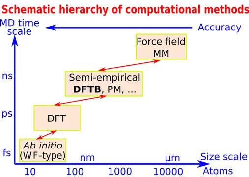
The empirical tight-binding methods (based on the limited atomic orbital basis-set representa-tion) have been developed in order to study large molecular systems.[114] _{Being roughly three}

orders of magnitude faster than DFT (see Figure 2.1), they contain a number of element-specific parameters. These parameters are generally transferrable (depending on the functional), but most importantly they allow tight-binding schemes to describe nearly all quantum effects accessible by DFT and Hartree-Fock methods.

Ab initio

10

100 1000

10000

DFT

Semi-empirical

DFTB, PM, ...

μm

nm

Force

MM

Accuracy

Atoms

MD time

scale

fs

ps

ns

Size scale

Schematic hierarchy of computational methods

ﬁeld

(W F -type)

Figure 2.1: Schematic hierarchy of computational methods in Quantum Chemistry. WF

stands for the wavefunction, PM is the parametric method, MD and MM stand for the molecular dynamics and molecular mechanics, respectively.

It was shown that a tight-binding scheme can be used as a basis for almost parameter-free approximate treatment within the DFT approach.[115]_{This led to the development of a Density}

Functional based Tight-Binding (DFTB) approach. The DFTB method was applied to study large molecules, clusters, nanoparticles and condensed-matter systems.[116,117]

(28)

18 2 Methods

First, one considers the electron density in Eqn. 2.6 as a sum of some reference density (e.g. sum of atomic densities) ρ0(r) and a small fluctuation δρ(r), i.e. ρ(r) = ρ0(r) + δρ(r). The

total energy (2.15) can be then expanded in a Taylor series up to a given order, leading to the following general equation

E[ρ0+ δρ] = E0[ρ0] + E1[ρ0, δρ] + E2[ρ0, (δρ)2] + E3[ρ0, (δρ)3] + . . . (2.20)

Finally, combining Eqn. 2.20with Eqn. 2.15and taking only terms with up to the second order of density fluctuations δρ, one can derive to the following equation for the total energy[118]

E = N ∑ i=1 ni⟨φi| ˆH0|φi⟩ − 1 2 ∫ ∫ _ρ 0(r)ρ0(r′) |r − r′_| drdr ′_{+ E} xc[ρ0] − ∫ ρ0(r)Vxc[ρ0(r)]dr + Enn+ +1 2 ∫ ∫ ( ₁ |r − r′_|+ ∂2_E xc ∂ρ∂ρ′ ρ=ρ0 ) δρ(r)δρ(r′)drdr′, (2.21) where ˆH0 = −∇2/2 + ˆVeff[ρ0].

Historically, DFTB models have been sequentially proposed and developed depending on the terms used in Eqn. 2.20, starting from the first-order non-self-consistent DFTB (DFTB0)[119,120]_,

followed by the second-order Self-Consistent Charge DFTB (SCC-DFTB or DFTB2)[121] _and

finally leading to the third-order DFTB[122]_{. Different implementations and extensions of DFTB}

are available within the following software packages: DFTB+[123]_{, deMon-Nano}[99]_{, ADF}[124]_,

Amber[125]_{, Gromacs}[126]_{, Gaussian}[127]_{, DFTBaby}[128] _{and CP2K}[129]_.

First-order DFTB

This approach neglects the last term in Eqn. 2.21. The DFTB is based on a LCAO ansatz (2.16) where atomic orbitals are obtained from the atomic DFT calculations in a confined potential[118]

and the basis is restricted to the valence shell to reduce the computational cost. The terms that depend on the reference density ρ0 and on the nuclear-nuclear repulsion Enn form the

pairwise, repulsive and short-ranged quantity denoted by Erep. The final energy expression for

the DFTB0 then reads

EDFTB0 = N

∑

i=1

ni⟨φi| ˆH0|φi⟩ + Erep, (2.22)

Within the DFTB0, KS equations (2.17) transform into the following system of algebraic equations using the set of localized atomic orbitals χµ= χµ(r − RA) ∀µ ∈ A

(29)

2.1 Density Functional Theory (DFT) 19

∑

ν

cνi(Hµν0 − εiSµν) = 0 ∀µ, i (2.23)

Now, using the fact that

N ∑ i=1 ni⟨φi| ˆH0|φi⟩ = N ∑ i=1 ni ∑ µν cµicνiHµν0 = N ∑ i=1 niεi; (2.24) Erep= 1 2 M ∑ A=1 M ∑ B=1 V_ABrep, (2.25) where Vrep

AB denotes the repulsive potential between pair of atoms A and B, the total DFTB0

can be written as follows[118]

EDFTB0 = N ∑ i=1 niεi+ 1 2 M ∑ A=1 M ∑ B=1 V_ABrep. (2.26)

The DFTB0 combined with the two-center approximation[115] _{allows to overcome the}

compu-tational bottleneck of DFT due to the fact, that Hamiltonian and AO overlap matrix elements (H0

µν and Sµν, respectively) as well as repulsive potentials Vrep can be calculated only once

for a set of interatomic distances between different elements. In practice, they are actually precomputed based on some reference electronic structure method (e.g. DFT with the LDA functional) and stored as an external datafile.

Second-order (Self-Consistent Charge) DFTB

The second-order DFTB scheme has been pioneered by Elstner et al. and published in 1998.[121]

The derivations presented below are rather concise and based on this original work.

In order to improve the charge balance in heteronuclear systems, the second order term in Eqn. 2.21has to be taken into account. First, the density fluctuation δρ is written as a superposition of atomic contributions δρA, i.e. δρ =∑_AδρA. The latter ones are further expanded in a series

of radial and angular functions and this expansion is truncated after the monopole term[121]

δρA(r) ≈ ∆qAF00A(|r − RA|)Y00≈ ∆qA FA 00(|r − RA|) √ 4π , (2.27) where FA

00 is the normalized radial dependence of the charge fluctuation ∆qA for quantum

numbers m = l = 0. Expression (2.27) preserves the total charge of the system, i.e. ∑_A∆qA=

∫

(30)

20 2 Methods ESCC = 1 2 ∫ ∫ ( ₁ |r − r′_|+ ∂2_E xc ∂ρ∂ρ′ ρ=ρ0 ) δρ(r)δρ(r′)drdr′ = = 1 2 M ∑ A=1 M ∑ B=1 ∫ ∫ Γ[r, r′, ρ0]δρA(r)δρB(r′)drdr′ = = 1 2 M ∑ A=1 M ∑ B=1 ∆qAγAB∆qB; (2.28) γAB = ∫ ∫ Γ[r, r′, ρ0]F A 00(|r − RA|)F00B(|r′− RB|) 4π drdr ′_. _(2.29)

In the limit of large interatomic distances, ESCC describes a non-screened Coulomb-type

interaction between two point charges ∆qA and ∆qB due to the vanishing exchange-correlation

contribution within the LDA. On the contrary, when both charges are localised on the same atom B, γBB≈ IPB− EAB ≈ UB, where UB is the Hubbard parameter, IPB and EAB denote

the atomic ionization potential and the electron affinity, respectively.[130]

Finally, the total DFTB2 energy takes the following compact form

EDFTB2 = N ∑ i=1 ni⟨φi| ˆH0|φi⟩ +1 2 M ∑ A=1 M ∑ B=1 ∆qAγAB∆qB+ Erep. (2.30)

Solving the secular KS equations (2.23) is no longer sufficient due to the fact that atomic charges depend on the molecular orbitals φi. Thus, a self-consistent procedure is required to

minimize the energy (2.30). But first, Mulliken charge analysis has to be applied to charge fluctuations[118] _∆q A= qA− ZA, i.e. qA= 1 2 N ∑ i=1 ni ∑ µ∈A M ∑ B=1 ∑ ν∈B

(c∗_µic_νiS_µν+ c_µic∗_νiS_νµ), (2.31) leading to the following set of KS equations for the Self-Consistent Charge (SCC) DFTB

∑ ν cνi(Hµν − εiSµν) = 0; ∀µ, i (2.32) Hµν = ⟨χµ| ˆH0|χν⟩ + 1 2Sµν M ∑ C=1 (γAC+ γBC)∆qC = Hµν0 + Hµν1 ; (2.33) Sµν = ⟨χµ|χν⟩ ∀µ ∈ A; ∀ν ∈ B (2.34)

An analytic expression has been derived for the interatomic forces by Elstner et al.[121]

FA= − N ∑ i=1 ni ∑ µν cµicνi [ ∂H0 µν ∂RA − ( εi− H1 µν Sµν ) ∂Sµν ∂RA ] − ∆qA M ∑ C=1 ∂γAC ∂RA ∆qC− ∂Erep ∂RA . (2.35)

(31)

2.2 Time-Dependent DFT(B) 21 The DFTB sets of parameters can be downloaded free of charge onwww.dftb.org. Among them, the matsci[131] _{(originally developed for Materials Science applications) and mio}[121] _(initially

parametrized for O, N, C and H) sets of parameters have been actively used for practical applications within both DFTB0 and SCC-DFTB approaches. However, several techniques have been recently proposed in order to improve the DFTB parametrization. In particular, the TANGO approach based on the SCC-DFTB coupled to the genetic algorithm has been developed for an enhanced global optimization.[132]_{Alternatively, unsupervised Machine Learning methods}

have been used to improve the fitting of repulsive potentials.[133]

Some limitations and extensions of the conventional DFTB

The DFTB approach has inherited all of the well-known drawbacks[134]_{of the conventional DFT.}

In particular,

• Poor description of weak interactions due to the lack of an explicit electron correlation. Dispersion correction has been originally proposed for the DFT total energy by Stefan Grimme[135] _{and has been later on integrated into some DFTB codes;}

• Absence of a wavefunction makes it problematic to access excited states that have the same symmetry as the ground state. However, excited state properties like energies, forces and transition dipole moments can be calculated within the linear response Time-Dependent DFT (TD-DFT) method, which was originally developed by Mark Casida[136]_{in 1995 and}

further adapted for DFTB by Niehaus et al.[86]_;

• Self-interaction error occurs due to the double counting of an electron-electron interaction in the DFT total energy expression, i.e.

1 2 ∫ ∫ ρ(r)ρ(r′₎ |r − r′_| drdr ′_{+ E} xc[ρ] ̸= 0. (2.36)

In particular, the long-range 1/r behaviour is not restored by conventional functionals (including LDA ones). However, this can be fixed by separation of the Coulomb interaction into the long-range and short-range contributions. This correction also improves the description of excited Rydberg states corresponding to the excitation of an electron into a diffuse orbital and charge-transfer states, where an electron is transferred over a large distance (e.g. intermolecular charge transfer). Two long-range corrected DFTB schemes have been proposed independently by Lutsker et al.[137]_{and Humeniuk and Mitrić}[138]_in

2015.

2.2 Time-Dependent DFT(B)

So far, all approximations and derivations concerned only ground state properties. The time has come to move towards the description of excited states, which is essential to describe many

(32)

22 2 Methods

relevant problems of molecular optics and electronic spectroscopy.

The Time-Dependent Density Functional Theory (TD-DFT) is an extension of the conventional DFT to the situation where a system in its ground stationary state is exposed to a time-dependent perturbation, which modifies its external potential.[136]_{A good overview of the}

TD-DFT fundamentals can be found in Ref. [139] .

Similarly to the original proof by Hohenberg and Kohn[41] _{for the ground state, Runge and}

Gross have demonstrated in 1984 the existence of a unique correspondence between the time-dependent electron density ρ(r, t) and the time-time-dependent potential ˆVeff[ρ(r), t].[140] This leads

to the following set of time-dependent KS equations

i∂φj(r, t) ∂t = [ −1 2∇ 2_{+ ˆ}_V eff[ρ(r), t] ] φj(r, t). (2.37)

In practice, Eqn. 2.37 has to be solved if the time-dependent potential is strong. It can be done within the Ehrenfest approach and is particularly useful for the real-time atomistic simulations of transient absorption spectroscopy.[141]_{On the other hand, in the limit of a weak}

perturbation, the linear response approximation can be applied to simplify the solution.[136] _In

the next section, I will introduce some basic linear response TD-DFT equations and will focus more on the tight-binding extension.

2.2.1 Linear Response TD-DFT(B)

The linear response only takes into account components of a density fluctuation δρ(r, ω) that depend linearly on the external perturbation, i.e.

δρ(r, ω) = ∫

χ(r, r′, ω)δVext(r′, ω)dr′, (2.38)

where δVext(r′, ω) is the linearized time-dependent KS potential from (2.14). The response

function χ of the non-interacting KS system is computed as a function of the stationary Kohn-Sham orbitals (complex conjugation is further suppressed for simplicity)

χ(r, r′, ω) = lim η→0+ N ∑ k=1 N ∑ l=1 (fk− fl) φl(r)φk(r)φl(r′)φk(r′) ω − (εl− εk) + iη , (2.39)

where fkis the Fermi occupation number of the KS molecular orbital k. Substituting (2.39) into

(2.38) and following the derivations from Ref. [136] , one arrives to the following non-Hermitian eigenvalue problem (Casida’s equation)[85]

( A B B A ) ( XI YI ) = ΩI ( 1 0 0 −1 ) ( XI YI ) , (2.40)

(33)

2.2 Time-Dependent DFT(B) 23 where ΩI = EI − E0 is the excitation energy corresponding to the vertical transition between

ground state E0 and excited state EI, 1 is the identity matrix, A and B are matrices with the

elements given by

Aia,jb= ωiaδijδab+ 2Kia,jb; (2.41)

Bia,jb= 2Kia,jb; (2.42)

and indices i, j and a, b denoting the occupied and virtual Kohn-Sham orbitals, respectively; ωia = εa− εi. Alternatively, the Tamm-Dancoff approximation has been introduced[142], which

neglects the B matrix, thus leading to the following equation

AXI = ΩIXI. (2.43)

The coupling matrix elements Kia,jb for singlet excited states are calculated in the adiabatic

approximation as follows[85,136] K_ia,jbS = ∫ ∫ φi(r)φa(r) [ 1 |r − r′_|+ ∂2_E xc ∂ρ(r)∂ρ(r′₎ ] φj(r′)φb(r′)drdr′. (2.44)

The TD-DFT approach was coupled to the DFTB by Niehaus et al. in 2001.[86]_{It required some}

additional approximations beyond the exchange-correlation functional in the coupling matrix Kia,jb. In the DFTB, both MOs and MO coefficients are real-valued, so I further suppress the

complex conjugation in order to be consistent with the literature. Similarly to the SCC-DFTB derivations, one has to decompose the transition density ρia _{= φ}

iφa into the atom-centered

contributions ρia

A, which are further expanded in series of radial and angular functions and

truncated after the monopole term[86]

ρia_A_{(r) ≈ q}ia_AF_A(r) (2.45)

where FA(r) is the normalized spherical density distribution and qiaA are the Mulliken atomic

transition charges, which can be computed as follows

qia_A = 1 2 ∑ µ∈A M ∑ B=1 ∑ ν∈B

(cµicνaSµν+ cµacνiSνµ). (2.46)

The coupling matrix (2.44) for singlet TD-DFTB excited states then reads[86]

K_ia,jbS = M ∑ A=1 M ∑ B=1 q_Aiaγ_ABqjb_B. (2.47)

(34)

24 2 Methods

For practical purposes, one can apply the following transformation (A −B)−1/2_(XI_{+ Y}I_{) = F}I

in Eqn. 2.40in order to derive the commonly used TD-DFT(B) set of equations

Ntr

∑

j→b

(ω2_iaδijδab+ 4√ωiaKia,jb√ωjb)FjbI = Ω2IFiaI. (2.48)

Since left-hand side in Eqn. 2.48 corresponds to a Hermitian matrix, eigenvectors FI _{form, in}

principle, an orthonormal basis set, i.e. ∑

I

FIFI = 1, (2.49)

which does not hold true for the eigenvectors of Eqn. 2.48. In particular, one can demonstrate that XI_XI _{− Y}I_YI _{= 1.}[85]

Singlet oscillator strengths[136]_{are important quantities of the optical spectra and can be easily}

computed within the TD-DFTB scheme[143]

fI = 4 3ΩI ∑ x,y,z Ntr ∑ i→a M ∑ A=1 R_Aq_Aia √ ωia ΩI F_iaI 2 (2.50) Triplet excited states can be computed as well within the TD-DFTB approach. This is achieved by introducing the following coupling matrix for triplet excited states[143]

K_ia,jbT =

M

∑

A=1

q_AiaM_Aqjb_A, (2.51)

where MA is the magnetic Hubbard parameter that can be obtained from the atomic DFT

calculations.[86]

The first application of the linear response TD-DFTB was reported by Niehaus et al. in Ref. [86]. Absorption spectra have been computed for neutral polyacenes ranging in size from naphthalene to heptacene. Excitation energies of the lowest and brightest excited singlet states are in good agreement with experimental and TD-DFT data. Later on, vibrationally resolved UV/Vis spectra of various aromatic and polar molecules were calculated using TD-DFTB excitation energies and analytical gradients.[144]_{The results of TD-DFTB are also in good agreement with}

the TD-DFT calculations using local functionals.

Some limitations and extensions of the conventional TD-DFT(B)

As has been shown before, the poor description of charge-transfer and Rydberg states is one of the major drawbacks of the linear response TD-DFT(B). However, there are some other limitations:

(35)

2.2 Time-Dependent DFT(B) 25 • Eqn. 2.48 is valid only for closed-shell systems. Spin-unrestricted TD-DFTB has been

developed in order to study the absorption spectra of open-shell complexes[145,146]_;

• The TD-DFT(B) is based on the linear response of the ground state, which may lead to an inappropriate description of the S1/S0 non-adiabatic coupling[128] and PES topology[147].

Thus, a proper description of dynamical processes that occur in the vicinity of the S1/S0

conical intersection (i.e. internal conversion to the ground state) remains challenging for methods based on the TD-DFT(B).

An extension of the DFTB (so-called DFTB-CI) has been developed by Rapacioli et al. for cationic molecular clusters.[148] _{It goes beyond the linear response formalism, thus eliminating}

all of the drawbacks presented above. This approach is based on the idea that a cluster can be described via a multiconfigurational wavefunction Ψ+

0 expanded on a basis of charge-localized

configurations Ψ+

ξ that correspond to removal of a single electron from the Highest Occupied

Molecular Orbital (HOMO) of the charged fragment ξ.

Even though it was initially developed to describe the ground state of charged molecular clusters, excited states can be extracted as well. A better description of the ionic excited states has been achieved through an extension of the original formalism. The expansion of a wavefunction is patched with additional terms[149]_{that correspond to removal of an electron from any occupied}

orbital of a charged fragment, i.e.

Ψ+₀ = Nfr ∑ ξ=1 occ ∑ i c_ξiΨ+_ξi. (2.52)

This modification becomes particularly important for clusters or stacks of large molecules with a small separation of occupied orbitals. Moreover, it allows to incorporate excited states that correspond to local excitations on the charged fragment and their coupling. This scheme has been shown to yield satisfactory PES of excited states in the full geometry range up to intermolecular dissociation of cationic PAH clusters.[149]

2.2.2 Analytical gradients for TD-DFT(B)

Molecular dynamics is a powerful tool that can be used to describe numerous physical and chemical processes. In order to propagate a classical trajectory on a given PES using Newton’s equations of motion, excited state energy gradients have to be developed for the linear response TD-DFT(B). Their derivation relies on the so-called Z-vector method, which was initially applied by Furche and Ahlrichs[150,151] _{to compute analytical forces within the TD-DFT}

approach. It was further adapted by Heringer et al.[152,153]_{to compute the TD-DFTB gradients.}

Alternatively, one can follow derivations of TD-DFTB gradients with the long-range correction from Ref. [128] .

(36)

26 2 Methods

Since ground state forces have been already developed by Elstner et al. for SCC-DFTB,[121]_,

one has to calculate only the gradient of the TD-DFTB excitation energy ΩI. However, this

is not a trivial task due to the fact that a straightforward calculation with finite differences is roughly 2Nf times more expensive than a single point DFTB calculation (here Nf denotes the

number of degrees of freedom).[152]_{One can also use a variational formulation of the TD-DFTB,}

which would require derivatives of the MO coefficients (roughly Nf times more expensive than a

single DFTB calculation), thus limiting the practical application of such gradients.[152]_{In order}

to avoid this computational bottleneck, an auxiliary Lagrangian has to be used:

L[X, Y, Ω, C, Z, W ] = G[X, Y, Ω] +∑ ia ZiaHia− ∑ p,q,p≤q Wpq(Spq− δpq), (2.53)

where G[X, Y, Ω] is a TD-DFT(B) functional[150] _{that leads to Eqn. (2.48). In this section,}

indices i, j, k and a, b, c denote occupied and virtual MOs, respectively, and p, q, r, s denote general MOs. In the equation above, quantities W and Z are Lagrange multipliers and their stationary conditions set restrictions on KS orbitals (e.g. that overlap Spq = δpq). The

stationarity of L with respect to MO coefficients C (∂L/∂Cµp = 0) leads to the so-called

Z-vector equation for an excited state I ∑

jb

(A + B)S_ia,jbZ_jbI = QI_ai_{− Q}I_ia. (2.54)

Blocks of the QI _{matrix has to be computed according to Appendix B from Ref. [152] and}

the corresponding erratum published in Ref. [153] . Once Eqn. (2.54) is solved, the WI _matrix

can be computed as well:

W_ijI = 1 1 + δij ( QI_ij+∑ kb 4K_ij,kbS Z_kbI ) ; (2.55) W_abI = 1 1 + δab QI_ab; (2.56) W_iaI = W_aiI = QI_ai+ ε_iZ_iaI. (2.57)

It is worth mentioning that the Z-vector itself contains valuable information about the nature of excited state. In particular, it has been used to investigate detachment/attachment processes characterizing a hole/particle pair generation upon an electronic transition in dyes.[154]

At the stationary point of L

L[X, Y, Ω, C, Z, W ] = Ω ⇒ _dRdL = dΩ

(37)

2.3 Non-adiabatic molecular dynamics 27 Since L is variational in all parameters, dL/dR = ∂L/∂R. Thus, the gradient of the excitation energy becomes dΩI dRA = ∂G ∂RA +∑ ia Z_iaI ∂Hia ∂RA − ∑ p,q,p≤q W_pqI ∂Spq ∂RA = =∑ ij T_ijI∂Hij ∂RA +∑ ab T_abI ∂Hab ∂RA + 2∑ ia ∑ jb (X + Y )I_ia(X + Y )I_jb∂Kia,jb ∂RA + +∑ ia Z_iaI ∂Hia ∂RA − ∑ p,q,p≤q W_pqI ∂Spq ∂RA (2.59)

Blocks of the TI _{matrix has to be computed according to Appendix B from Ref. [152] and}

the corresponding erratum published in Ref. [153] . In the equation above, vector elements (X + Y )I

ia are computed as follows

(X + Y )I_ia= √ εa− εi ΩI F_iaI, (2.60) where FI

ia is the eigenvector of (2.48). At this point, one can switch to the AO basis in order to

take advantage of derivative terms that have been already computed for the ground state forces (2.35). The AO to MO transformation can be done as follows

∂Spq ∂RA =∑ µν CµpCνq ∂Sµν ∂RA . (2.61)

Finally, the gradient of the excitation energy on atom A reads dΩI dRA =∑ µν P_µνI ∂Hµν ∂RA − ∑ µν W_µνI ∂Sµν ∂RA + 2 ∑ µνλσ (X + Y )I_µν(X + Y )I_λσ∂Kµν,λσ ∂RA , (2.62)

where PI _{= T}I _{+ Z}I _{is the one-particle difference density matrix and H}

µν is the SCC-DFTB

Hamiltonian matrix element from (2.33).

2.3 Non-adiabatic molecular dynamics

Standard molecular dynamics usually relies on the Born-Oppenheimer approximation, which retains a single adiabatic electronic state in the expansion of a wavefunction of the system. Several approaches have been developed in recent years to incorporate the non-adiabatic effects both at the ab initio[61] _{and mixed quantum-classical}[62–64,73] _{levels of theory. Nowadays, one}

of the most commonly used quantum-classical method is the Tully’s Fewest-Switches trajectory Surface Hopping (FSSH)[83,84]_{, which is based on the assumption that the nuclear wavepacket}