HAL Id: tel-01622934
https://pastel.archives-ouvertes.fr/tel-01622934
Submitted on 24 Oct 2017HAL is a multi-disciplinary open access
archive for the deposit and dissemination of sci-entific research documents, whether they are pub-lished or not. The documents may come from teaching and research institutions in France or abroad, or from public or private research centers.
L’archive ouverte pluridisciplinaire HAL, est destinée au dépôt et à la diffusion de documents scientifiques de niveau recherche, publiés ou non, émanant des établissements d’enseignement et de recherche français ou étrangers, des laboratoires publics ou privés.
Rule-Based Systems
Olivier Wang
To cite this version:
Olivier Wang. Adaptive Rules Model : Statistical Learning for Rule-Based Systems. Machine Learning [cs.LG]. Université Paris-Saclay, 2017. English. �NNT : 2017SACLX037�. �tel-01622934�
Thèse de doctorat de l’Université
Paris-Saclay préparée à l’École
Polytechnique
École doctorale n°580 : Sciences et Technologies de l’Information et de la
Communication (STIC)
Spécialité de doctorat : Informatique
ParM. Olivier
Wang
Adaptive Rules Models: Analytics Learning for
Rule-Based Systems
Thèse soutenue et présentée à Palaiseau, le 28 juin 2017
Composition du jury :
Mme. Ioana Manolescu, Directrice de Recherche Président
LIX - INRIA
M. Adrian Paschke, Professeur Rapporteur
Freie Universität Berlin
M. Marco Gavanelli, Professeur Associé Rapporteur
Université de Ferrare
Claudia D’Ambrosio, Maître de Conférences Examinateur
LIX - INRIA
Mme. Catherine Faron Zucker, Maître de Conférences Examinateur
Université de Nice Sophia Antipolis
M. Nicolas Changhai Ke, Architecte Produit BRMS Examinateur
IBM France
M. Leo Liberti, Directeur de Recherche Directeur de thèse
Business Rules (BRs) are a commonly used tool in industry for the automation of repetitive decisions. The emerging problem of adapting existing sets of BRs to an ever-changing environment is the motivation for this thesis. Existing Supervised Machine Learning techniques can be used when the adaptation is done knowing in detail which is the correct decision for each circumstance. However, there is currently no algorithm, theoretical or practical, which can solve this problem when the known information is statistical in nature, as is the case for a bank wishing to control the proportion of loan requests that its automated decision service forwards to human experts. We study the specific learning problem where the aim is to adjust the BRs so that the decisions are close to a given average value.
To do so, we consider sets of Business Rules as programs. After formalizing some definitions and notations in Chapter 2, the BR programming language defined this way is studied in Chapter 3, which proves that no algorithm exists to learn Business Rules with a statistical goal in the general case. We then restrain the scope to two common cases where BRs are limited in some way: the Iteration Bounded case in which no matter the input, the number of rules executed when taking the decision is less than a given bound; and the Linear Iteration Bounded case in which rules are also all written in Linear form. In those two cases, we later produce a learning algorithm based on Mathematical Programming which can solve this problem. We briefly extend this theory and algorithm to other statistical goal
learning problems in Chapter 5, before presenting the experimental results of this thesis in Chapter 6. The latter includes a proof of concept to automate the main part of the learning algorithm which does not consist in solving a Mathematical Programming problem, as well as some experimental evidence of the computational complexity of the algorithm.
Although the algorithms used in Business Rules management systems have been studied and compared, the theoretical study of BR as a programming lan-guage has not attracted interest from the research community before now. We dedicate Chapter 3 to this study. We prove the Turing-completeness of this lan-guage, which is often assumed but was never proven before, to the best of our knowledge. Of the two proofs we provide, we use the constructive proof to define a canonical equivalence between BR programs and WHILE programs. We use the WHILE form of BR programs to describe a Structural Operational Semantics for BR programs, and showcase the usefulness of this semantics by using it to prove the termination of some BR programs. The last property of BR programs we prove in that chapter has a proof based on the Turing-completeness of BR programs and answers part of the question which motivated this thesis: there is no algorithm which learns Business Rules with a statistical goal in the general case.
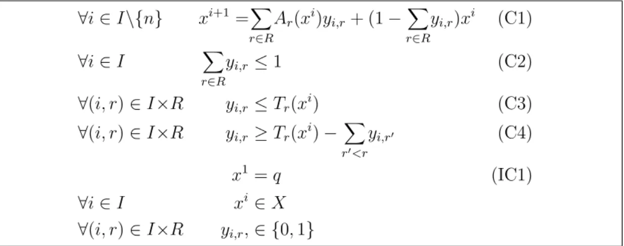
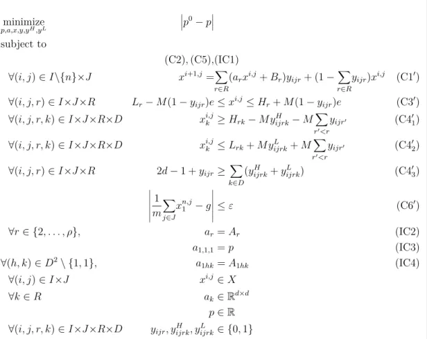
The contents of Chapter 4 alternate definitions and algorithms. We describe It-eration Bounded Business Rules (IBBR) programs, which are such that the number of Business Rules executed to take any given decision is bounded by a known value. We exhibit a Mixed-Integer Programming (MIP) problem such that, for IBBR pro-grams, solving it is equivalent to solving the statistical goal learning problem. Sim-ilarly, we describe Linear Iteration Bounded Business Rules (LIBBR) programs, which are Iteration Bounded Business Rules programs such that the Business Rules follow a given linear template. The associated algorithm produces a Mixed-Integer Linear Programming (MILP) problem. We evaluate the theoretical complexity of
this algorithm.
We extend the formalism and learning algorithms presented so far to a different class of learning problems in Chapter 5. We exhibit a Mathematical Programming equivalent to LIBBR programs in the case where the known information is over a quantized frequency distribution of the decisions taken, rather than over the aver-age decision taken. In two specific such cases, that of the distribution respecting an upper bound on the frequency of a specific decision and that of the distribution being almost uniform, we also exhibit a MILP problem which is equivalent when the BR program is a LIBBR program.
In Chapter 6, we provide the proof of concept showing how our learning algo-rithm can be automated to be integrated into a BR management software. The numerical part of our experimental work is in turn entirely dedicated to evaluat-ing the MILP obtained from a LIBBR program usevaluat-ing the algorithm described in Chapter 4. The evidence obtained shows that this direct application cannot be scaled up to industrial BR programs. We evaluate the validity of our algorithm by testing the number of randomly generated BR programs that our algorithm can solve. We also evaluate the performance by varying different characteristics of the learning problem and observing the CPU time taken by a standard Mathematical Programming solver to solve the learning problem.
Les Règles Métiers (Business Rules en anglais, ou BRs) sont un outil communé-ment utilisé dans l’industrie pour automatiser des prises de décisions répétitives. Le problème de l’adaptation de bases de règles existantes à un environnement en constante évolution est celui qui motive cette thèse. Des techniques existantes d’Apprentissage Automatique Supervisé peuvent être utilisées lorsque cette adap-tation se fait en toute connaissance de la décision correcte à prendre en toutes circonstances. En revanche, il n’existe actuellement aucun algorithme, qu’il soit théorique ou pratique, qui puisse résoudre ce problème lorsque l’information con-nue est de nature statistique, comme c’est le cas pour une banque qui souhaite contrôler la proportion de demandes de prêt que son service de décision automa-tique fait passer à des experts humains. Nous étudions spécifiquement le problème d’apprentissage qui a pour objectif d’ajuster les BRs de façon que les décisions prises aient une valeur moyenne donnée.
Pour ce faire, nous considérons les bases de Règles Métiers en tant que pro-grammes. Après avoir formalisé quelques définitions et notations dans le Chapitre 2, le langage de programmation BR ainsi défini est étudié dans le Chapitre 4, qui prouve qu’il n’existe pas d’algorithme pour apprendre des Règles Métiers avec un objectif statistique dans le cas général. Nous limitons ensuite le champ d’étude à deux cas communs où les BRs sont limités d’une certaine façon : le cas Borné en Itérations dans lequel, quelles que soient les données d’entrée, le nombre de règles
exécutées en prenant la décision est inférieur à une borne donnée ; et le cas Linéaire Borné en Itérations dans lequel les règles sont de plus écrites sous forme Linéaire. Dans ces deux cas, nous produisons par la suite un algorithme d’apprentissage basé sur la Programmation Mathématique qui peut résoudre ce problème. Nous étendons brièvement cette formalisation et cet algorithme à d’autres problèmes d’apprentissage à objectif statistique dans le Chapitre 5, avant de présenter les résultats expérimentaux de cette thèse dans le Chapitre 6. Ce dernier inclut une preuve de concept pour l’automatisation de la partie principale de l’algorithme d’apprentissage qui n’est pas celle où l’on résout un problème de Programmation Mathématique, ainsi que des indications expérimentales sur la complexité compu-tationelle de l’algorithme.
Bien que les algorithmes utilisés dans les systèmes de gestion des Règles Métiers aient été étudiés et comparés, l’étude théorique des BRs en tant que langage de pro-grammation n’a pas attiré l’intérêt de la communauté scientifique jusqu’à présent. Nous dédions le Chapitre 3 à cette étude. Nous prouvons la Turing-complétude de ce langage, qui est souvent supposée vraie mais n’a jamais été prouvée à ce jour, autant que nous le sachions. Des deux preuves que nous fournissons, nous utilisons la preuve constructive pour définir une équivalence canonique entre les programmes BR et les programmes WHILE. Nous utilisons la forme WHILE des programmes BR pour décrire une Sémantique Opérationnelle Structurelle pour les programmes BR, et mettons en évidence l’utilité de cette sémantique en l’utilisant pour prouver la terminaison de quelques programmes BR. La dernière propriété des programmes BR que nous prouvons dans ce chapitre a une preuve basée sur la Turing-complétude des programmes BR et répond à une partie de la question qui a motivé cette thèse : il n’existe pas d’algorithme qui apprend les Règles Métiers avec un objectif statistique dans le cas général.
y décrivons les programmes de Règles Métiers Bornés en Itérations (Iteration Bounded Business Rules en anglais, soit IBBR), qui sont tels que le nombre de Règles Métiers exécutées pour prendre une décision donnée est borné par une valeur connue. Nous exhibons un problème de Programmation Mixte en Nom-bres Entiers (Mixed-Integer Programming en anglais, ou MIP) tel que le résoudre soit équivalent, pour un programme IBBR, à résoudre le problème d’apprentissage à but statistique. De la même façon, nous décrivons les programmes de Règles Métiers Linéaires Bornés en Itérations (Linear Iteration Bounded Business Rules en anglais, soit LIBBR), qui sont des programmes IBBR tels que les Règles Métiers suivent un modèle linéaire donné. L’algorithme associé produit un problème de Programmation Linéaire Mixte en Nombres Entiers (Mixed-Integer Linear Pro-gramming en anglais, ou MILP). Nous évaluons la complexité théorique de cet algorithme.
Nous étendons le formalisme et les algorithmes d’apprentissage présentés jusque là à une classe de problèmes d’apprentissages différente dans le Chapitre 5. Nous exhibons un équivalent en Programmation Mathématique aux programmes LIBBR dans le cas où l’information connue couvre une distribution quantisée des décisions prises, plutôt que la moyenne des décisions prises. Dans deux cas spécifiques, celui où la distribution respecte une borne supérieure sur la fréquence d’une décision par-ticulière et celui où la distribution est presque uniforme, nous exhibons également un problème MILP qui est équivalent lorsque le programme BR est un programme LIBBR.
Dans le Chapitre 6, nous produisons une preuve de concept qui montre com-ment notre algorithme d’apprentissage peut être automatisé pour être intégré dans un logiciel de gestion de BR. La partie numérique de notre travail expérimental est quant à elle dédiée entièrement à l’évaluation du MILP obtenu à partir d’un pro-gramme LIBBR en utilisant l’algorithme décrit dans le Chapitre 4. Les indications
obtenues montrent que cette application directe ne peut pas être mise à l’échelle pour s’appliquer à des programmes BR industriels. Nous évaluons la validité de notre algorithme en testant le nombre de programmes BR générés aléatoirement que notre algorithme peut résoudre. Nous évaluons également la performance en faisant varier différentes caractéristiques du problème d’apprentissage et en obser-vant le temps CPU qu’un solver de Programmation Mathématique standard met à résoudre le problème d’apprentissage.
First and foremost, I would like to thank my advisor Prof. Leo Liberti, who has followed, pushed and supported my work for the whole length of my PhD study. His sincere wish to have me produce the best research possible made all of this thesis possible. I could not have had better advisor for my PhD study.
Special thanks also go to my supervisors at IBM. My administrative supervisors M. Patrick Albert, who pushed for IBM to fund this PhD and recruited me, and his successor M. Christian De Sainte Marie, who guided me during my research and the writing of this thesis, were both essential to the success of my thesis.
I am grateful to all the members of my thesis committee. Prof. Adrian Paschke and Prof. Marco Gavanelli did a wonderful work as referees – their comments have led to improvements in the text of this thesis in many places, notably in Chapter 1. Prof. Ioana Manolescu and Prof. Catherine Faron Zucker were wonderful members of the jury with insightful comments and questions. Prof. Claudia D’Ambrosio was all that and more, as she also helped with the Mathematical Programming part of my PhD study. M. Changhai Ke was also my scientific supervisor at IBM, and helped me explore the potential of Business Rules both during my thesis and my defense.
A big thank you also to the rest of the team at the LIX: Sonia, Raouia, Claire, Pierre-Louis, Gustavo, Luca, Ky, Youcef, all of you were great friends and co-workers. Special mention to Pierre-Louis and Sonia for helping with brainstorming
sessions and to Gustavo for giving me tips about the LIX servers and the thesis formatting! I cannot forget grouchy Evelyne either, our ever-busy and ever-helpful secretary, she is a marvel.
This thesis would not have been the same without my fellow PhD students at IBM either. Oumaima, Karim, Hamza, Nicolas, Penelope, and Reda, we experi-enced the wonders of working on a thesis at the IBM lab together, and I would not have it any other way.
Last but not least, I thank all the friends and family who supported me through this thesis: my friends Eric and France (and their cat Styx), my brother and sister, my parents, and my wonderful girlfriend Isabelle. You all bring joy to my life, and I love you.
Glossary xiii
1 Introduction 1
1.1 Motivation . . . 2
1.2 The contributions . . . 3
1.3 The approach . . . 4
2 Definitions and state of the art 6 2.1 Business Rules (BRs) . . . 6
2.1.1 BRs in industry and research . . . 7
2.1.2 A formal definition of BRs . . . 12
2.2 Machine Learning (ML) . . . 27
2.2.1 Statistical goal learning . . . 30
2.2.2 Computational Learning theory . . . 34
2.3 Mathematical Programming (MP) . . . 36 2.3.1 MP formalism . . . 37 2.3.2 MP solvers . . . 38 3 BR programs 40 3.1 Turing-Completeness of BR programs . . . 41 3.1.1 Turing-Completeness . . . 43 x
3.1.2 Basic Turing-completeness Proof . . . 43
3.2 Constructive proof and resulting Operational Semantics . . . 47
3.2.1 BR form of WHILE programs . . . 47
3.2.2 WHILE form of BR programs . . . 53
3.2.3 A Structural Operational Semantics for BR programs . . . . 55
3.3 Learnability of the statistical goal learning problem . . . 63
3.3.1 PAC-Learnability . . . 63
3.3.2 Complete unlearnability . . . 65
4 MP based algorithm 69 4.1 General Iteration Bounded BR programs . . . 70
4.1.1 IBBR programs in two BR languages . . . 70
4.1.2 Complexity of IBBR programs . . . 73
4.1.3 Declarative form of an IBBR programs . . . 74
4.2 A learning algorithm: MP . . . 77
4.3 Linear Iteration Bounded BR programs . . . 81
4.3.1 Linear BR programs . . . 81
4.3.2 Example: Decision Trees . . . 84
4.4 An algorithm for LIBBR programs . . . 86
4.4.1 A learning algorithm: MIP . . . 88
4.4.2 A learning algorithm: MILP . . . 90
4.5 Theoretical complexity . . . 93
5 General statistical goal learning 95 5.1 Learning quantized distributions . . . 97
5.2 Upper bound on a specific output value’s probability . . . 98
6 Experimental work 103
6.1 Parsing ODM . . . 104
6.2 Experimental data on learning LIBBR . . . 108
6.2.1 Experimental setup . . . 108
6.2.2 Validating the learning algorithm . . . 109
6.2.3 Testing performance . . . 111
6.2.4 Testing other statistical goal learning problems . . . 115
7 Discussion 132 7.1 A formal study of BRs . . . 133
7.2 New learning algorithms . . . 134
7.3 Industrial applications . . . 135
7.4 Conclusion . . . 137
A Complete proof of some theorems 139 A.1 Complete proof of Theorem 4.8 . . . 139
A.2 Complete proof of Theorem 4.9 . . . 143
BR Business Rules
BRMS Business Rules Management System IBBR Iteration Bounded Business Rule(s) iff if and only if
LIBBR Linear Iteration Bounded Business Rules(s) MIP Mixed-Integer Programming
MILP Mixed-Integer Linear Programming MINLP Mixed-Integer Nonlinear Programming ML Machine Learning
MP Mathematical Programming ODM Operational Decision Management PAC Probably Approximatively Correct POC Proof of Concept
PRF Pseudorandom Function
SOS Structural Operational Semantics TM Turing Machine
UTM Universal Turing Machine
Introduction
This thesis is concerned with tuning parameters in Business Rules programs so that a given statistical measure over all the decisions taken by a given Business Rules (BR) program satisfies a given objective. Business rules are used in industry today as a functional way to formally encode corporate policies and regulations. For example, the decision of whether to grant a loan request, refuse it, or mark it for further review by a human expert is often made by a BR program. Of course, the decision should be made on a per-customer basis, and yet there may be reasons on a corporate scale to wish for a certain proportion of all loans to be reviewed by human experts, while the rest can be treated automatically. We investigate how the rules in a BR program can be tuned automatically, e.g. to adapt to changes in the reviewing policy or to evolutions in the market.
In this introduction, we first explain the reasons motivating this thesis, then we outline the main contributions of this thesis, including publications. Finally, we give an overview of the methodology followed in this manuscript.
1.1
Motivation
This PhD was sponsored by IBM France Lab, the R&D unit in IBM which is responsible for the development and support of IBM Operational Decision Man-agement (ODM), one of the most popular Business Rules ManMan-agement System (BRMS) on the market [57]. A very common request clients make to the ODM support team is help in creating a BR program which outputs the correct deci-sions for the example inputs they already have, while keeping the structure of the rules modeled by their business experts. The defining characteristics of a correct decision differ from client to client.
The main motivation for this thesis was the realization that many of IBM’s clients have a statistical definition of what makes a decision model ‘correct’. No tool or theory exists to parametrize an existing BR program with the objective of “thirty percent of decisions must be reviewed manually over the example cases”. Studying the possibility and practicality of creating such a tool is the main objec-tive of this thesis from the point of view of IBM.
Outside the specific environment of BRMS vendors such as IBM, other situ-ations also call for this type of statistical parametrization. In many situsitu-ations, the existence of an algorithm for learning a program with a statistical goal would be very practical, as is the case in the medical field when trying to match ADN sequences and genetic predisposition to illnesses. Learning statistical goals is a problem with many important industrial applications, yet little formal research. In this thesis, we explore a possible solution to this problem when applied to BR programs.
1.2
The contributions
During this thesis, we have proved that no algorithm can ever guarantee an exact conformance to given statistics over all possible cases: the task of learning the behavior of BR programs in general is formally impossible. This general result does not prevent some subset of BR programs to be learnable, including some that are of particular interest to us: BR programs that have a bounded execution time and BR programs that have only linear rules. This result stems from the Turing-completeness of the BR programming language, which is widely known yet had avoided published formal proof for a long time.
From the Turing-completeness of the BR programming language, we have de-scribed a WHILE form of BR programs which we used to define a Structural Operational Semantics (SOS) for BR programs. We have shown that this SOS can be used to prove properties of BR programs such as termination over a range of inputs.
The most relevant result for out initial research question is the creation of a learning algorithm for the statistical goal learning problem applied to Iteration-Bounded BR (IBBR) programs. This algorithm based on Mathematical Program-ming can be used to transform a statistical goal learning problem into Mixed-Integer Linear Problems (MILPs) in the case of Linear IBBR (LIBBR) programs. We have applied this algorithm and evaluated its algorithmic complexity using em-pirical solving times obtained with a standard MILP solver. We have also extended the original algorithm to different statistical goals that the one it was originally created for, and used it to solve two additional types of statistical goal learning problems.
The theoretical impossibility result was published with a formal proof of the Turing-completeness in [140]. The description and testing of the original learning algorithm was published in [138]. The general statistical goal learning problem
and the extension of the algorithm to different statistical goals was published in [139].
1.3
The approach
In Chapter 2, we define the notions and notations which will be used in the rest of this thesis, and present the existing research relevant to our work in the domains of Business Rules, Machine Learning and Mathematical Programming. We notably present a formal definition of Business Rules in Sec. 2.1, then a formal definition of the statistical goal learning problem in Sec. 2.2.
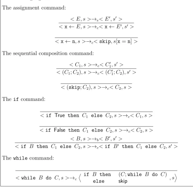
We then seek to answer the question of the existence of an algorithm which can solve the learning problem of interest in this thesis, that of learning parameters of a BR program when given a statistical goal, in the general case. Chapter 3 is dedicated to studying this question. We give a negative answer in Sec. 3.1 by proving the Turing-compleness of BR programs, and derive a useful operational semantics for BR programs from our proof. This operational semantics can in particular be used to prove termination of a BR program over an interval of values, by encoding the BR semantics into an inference engine such as Prolog [99], as demonstrated in Subsec. 3.2.3. We then further generalize the nonexistence of a learning algorithm in Sec. 3.3 by proving not only PAC-unlearnability, but an even stronger unlearnability property.
In the rest of the thesis, we study a MP-based algorithm for solving the sta-tistical learning problem when restricted to some subclasses of BR programs. We introduce Iteration Bounded BR programs (IBBR) and Linear Iteration Bounded BR programs (LIBBR) in Chapter 4. In each case, we provide an equivalent MP problem to the learning problem formalized in Sec. 2.2. We show that this problem can be solved for a LIBBR program by a MILP solver in Sec. 4.4.
We briefly touch on different forms of statistical learning problems in Chapter 5. In particular, we provide MP formulations for two different problems: the problem where the proportion of outputs taking a particular value (e.g. o1) is bounded, i.e. card({q ∈ Q | P (p, q) = o1})/card(Q) ≤ g, and the problem where the outputs must respect an almost uniform distribution. Those formulations are also MILP problems when the BR programs are LIBBR programs.
We also cover some practical tests to evaluate the practicality of our algorithm in Chapter 6. We include a practical way of creating the MILP problem for a BR program written with IBM Operational Decision Management (ODM), as well as a few tests on the different forms of statistical learning problems.
We conclude this thesis with a discussion of our contributions and of the re-search perspectives this work opens in Chapter 7.
Definitions and state of the art
In this Chapter we introduce the three key concepts which we make use of in this thesis: Business Rules (BRs), Machine Learning (ML), and Mathematical Pro-gramming (MP). In the first section, we introduce the notion of Business Rules used in industry and research, then formally define BR programs. In the second section, we formalize our learning problem and relate our problem to conventional Machine Learning theory. The third section introduces Mathematical Program-ming definitions and conventions, as MP is the main component of the learning algorithm introduced in this thesis.
2.1
Business Rules (BRs)
BRs are a rules-based programming language in which writing a program consists of defining rules such as “If the person requesting this loan has negative balance on a bank account, Then refuse this loan request and watch that account”. BRs are very popular in corporate environments as a way of automating decision man-agement.
In this section, we first informally explore the uses of BRs in industry and
research, and how they relate to this thesis. We then formally define BR programs and their interpreters, and we justify the simplifications used in the rest of the thesis compared to the BR execution algorithms used in commercial products.
2.1.1
BRs in industry and research
Any organization, from the smallest start-up to the largest governmental agency, must constantly make decisions of all kinds, from the most convoluted budget assignment to the simplest YES/NO binary choice. Automated decision manage-ment has existed for years as a way to save time and rationalize some of the most repetitive decisions an organization must take. This mostly applies to large com-panies which have well-defined business policies to be applied in circumstances where either traceability or compliance is needed.
Used for automated decision management, Business Rules are a popular way of modeling operational decisions, such as generating quotes for insurance com-panies, transaction processing for financial comcom-panies, or price computation in retail. Business Rules Management Systems (BRMS) such as IBM Operational Decision Management (ODM), previously known as ILOG JRules, are used by corporations of all sizes to let business experts automate their expertise while still using an easily understandable approximation of natural language [91]. BRMS are commercialized in multiple forms, which also include FICO Decision Management Suite [42], TIBCO Business Process Management Suite [123], Pega Robotic Pro-cess Automation [96], RedHat JBoss BRMS [61], OpenRules [93], and ServiceNow [112], and others. The Java Rules engine JESS [62] also sees some industrial use. One of the most popular characteristics of BRMS is their ease of use: business processes are defined by business analysts who do not often have a Computer Sci-ence background, which justifies the choice of BRs – as a “programming language for non-programmers” – to encode the decisions which are part of those processes.
This ease of use stems from the fact that BRs have a streamlined syntax which makes writing BR programs as elegant as declarative programming languages. This characteristic is emphasized by using pseudo-natural language to bridge the gap between the machine definition of objects (both classes and methods) and their business definition. Every sector of business can find uses for BRMS, from banks (e.g. for loan validation) to car companies (e.g. for car models and options pricing) to insurance companies (e.g. for fraud detection).
The primary strength of BRs compared to other decision management sys-tems lies in its agility. As business environments change, business policies must inevitably adapt. It has become increasingly frequent due to globalization, which accelerates regulation and market changes. Organizations have to conform with more and more regulations, market demand evolves faster and faster, and com-petition reacts and must be reacted to with increasingly short delays. BRMS allow business experts with no advanced computer knowledge to write and modify BRs, after the initial intervention of the I.T. department to devise semi-natural, domain-specific rule languages. Furthermore, BRMS include practical lifecycle management of BR programs such as modifying BRs which are already deployed to production, along with the usual versioning and collaborative working features. The initial idea which later led to BRs appeared under the name of Production Rules in the 1970s as a knowledge representation system [37] originating as a psy-chological model of human reasoning behavior [85, 86]. In the 1980s, the Artificial Intelligence research community implemented the knowledge representation sys-tem used in Production Rules as defined by the modeling community into Expert Systems. They were first theorized [29, 74] then implemented in expert systems such as R1 [143], MYCIN [21, 83], EMYCIN [21, 40], or OPS5 [94, 95]. OPS5 in particular was based on the Rete algorithm [43], which is still in use in many BRMS today. The commercial successors of OPS5 included CLIPS [30], Jess [62],
Nexpert [87], and ILOG Rules [59], which evolved into the BR engine currently used by ODM.
As the popularity of Expert Systems faded, the utility of Production Rules as a business decision modeling tool was quickly apparent to the business community, where they gained the name of Business Rules. Although Ronald Ross wrote the very first book about business rules in 1994 [107] and claims to be “the father of business rules” [108], a number of other authors contributed to the definition and expanded use of business rules as an approach to representing business knowledge [53, 54, 18], going as far back as Knolmayer in 1993 [68]. Methodologies have been defined, in particular the Business Rules Manifesto by the Business Rules Group [19].
Expert Systems were progressively replaced by the current form of BRMS, as the decline in popularity of Expert Systems led to the use of standardized BR engines as direct implementations of BRs as defined by the business modeling community: where once Rules engines aimed to intelligently produce a handful of strategic or expert decisions, they now automate thousands of operational and routine decisions.
The defining characteristics of BRMS which any further improvement must take into account and respect are thus automation – the ability to apply one specified action to any number of relevant examples – and accessibility – an ease of use which can allow a Business Analyst to use the interface without issue. The goal of this thesis is to investigate the use of Machine Learning (ML) to modify BRs in an automated fashion. This would allow BRMS to combine their natural advantage – the ease of programming which makes them understandable by business experts – with their ML competitors’ best advantage – the ability to take advantage of the vast amounts of data naturally produced by businesses in the age of the Internet. Rules related programming languages in computer science today can broadly
be separated in two categories, which must not be confused [136]:
• Inference systems are closest to logic programming languages, they use Logic Rules and allow for both forward and backward chaining to deduce facts or prove theorems given rules and facts. Prolog [99] is an example of rule-based inference system. Datalog [36] can also be used as a query language for deductive databases. Logic Rules are also used in constraint programming, e.g. in the form of Constraint Handling Rules [27].
• Production systems are closest to standard imperative programming lan-guages, they use Production Rules which can dynamically affect the value of variables at execution time. In query languages such as Datalog¬¬ [1], which use inference engines, this means allowing for negations in heads of rules, in-terpreted as deletions of facts. In expert systems such as OPS5 [94], which use production engines, this means using assignment operations. In terms of logic programming, the presence of assignments means that inference in production systems can be non-monotonic.
The Business Rules we study are part of the second family, they have side effects which in turn affect the conditions of other rules, thus making logical inference impractical (in particular backwards chaining).
Inference systems have been explored in many different ways. Multiple infer-ence languages exist [1] with different reasoning systems, which allow backward chaining, forward chaining, and negation as failure to different degrees. While our focus is not on Logic Rules, it must be noted that many applications of Rules systems use Logic Rules rather than Production Rules – or rather, they fall into the overlap which consists of two functionally equivalent classes of Rule systems: Business Rules where actions do not modify existing variable values; and Logic Rules which only consider forward chaining, with neither backward chaining nor
negation as failure. One such example is the research in using a rule-based repre-sentation system to organize and execute legal reasoning [71, 70].
Recent research in Production Rules systems has been mostly limited to their applications as a knowledge representation method, such as in [110]. An important part of that focus is dedicated to the combination of Production Rules and Ontolo-gies, as two complementary and synergistic knowledge representations methods: Production Rules focus on the description and execution of business logic while Ontologies focus on the description and structure of domain knowledge [92, 82, 8]. This has led to the SWRL standard proposal [122], which combines the OWL on-tology format with the RuleML rules format. Other areas of research in Production Rules systems include handling uncertainty [2] and automated explanation.
We choose to focus on BRs as a commonly used way of encoding business knownledge and automating decisions [46, 58] of interest to IBM. While Produc-tion Rules can be represented by declarative logic programs [105, 119], such a transformation does not bring us closer to a learning algorithm for our problem: existing Logic Rules learning algorithms aim to learn relationships, in the fash-ion of associatfash-ion rule learning (see Sec. 2.2). As we are trying to refine existing BR programs so as to satisfy a statistical goal, we wish to learn parameters in Production Rules rather than to learn Rules themselves, which makes relationship learning irrelevant to our research.
To avoid confusion, we hereafter call Business Rules (BRs) the constituents of a computer program meant to be executed by a BRMS or similar BR execution engine, while what is called a business rule by the Business Rules Group is referred to explicitly as a business modeling rule when necessary. In the example from
earlier, the business modeling rule
“Loan requests made while the borrower has a negative balance on one of his bank accounts are to be refused, and such accounts must then be watched”
might be decided by a business analyst. Such rules can be written in natural language using an if-then template:
If the person requesting this loan has negative balance on a bank account,
Then refuse this loan request and watch that account
(2.1)
In this example, the phrase “the person requesting this loan has negative balance on a bank account” is the condition, and the phrase “refuse this loan” is the action associated with this business modeling rule. A set of such rules can be written as a BR program given an appropriate representation of the business objects referred to in business modeling rules, e.g. as a well-defined set of objects and classes, called a Business Object Model in ODM.
2.1.2
A formal definition of BRs
The origin of BRs as a knowledge representation system and the later focus on implementations of BRs as business tools have lead to a lack of studies on BRs as a programming language. That is the starting point we choose to use for the contributions in this thesis. A BR is an if-then statement in which if is followed by a boolean expression, called the condition, and then is followed by a sequence of assignment instructions, called the action1. This action can include non monotonic
1 In practice, actions can include all sorts of instructions. However, we disregard
effects, unlike the consequence clause of Logic Rules.
The syntax of BRs is straightforward, as it is aimed at non-programmers. In particular, it avoids explicit occurences of loops and function calls, which non-programmers may find difficult to understand. BRs eliminates the need for explicit loops – by making them implicit in the interpreter – and can fulfill the role of function calls (code factorization) by using what we call in this thesis typed
meta-variables.
Most BRMS use typed meta-variables to simplify their users’ task. We explain how those work, then show that the expressive power of such a BR programming language is the same as one that does not use meta-variables at all.
In the rest of this thesis, we often use self-explanatory pseudo-code to describe programming language behavior. The use of the keywords if ... then .. end if, while ... do ... end while, True and False as well as the function type() and the symbol
← do not refer to a specific implementation of computer instructions, but rather
to familiar concepts of computer science, namely if-then statements, while loops, Boolean values, variable type evaluation and affectation of a value to a variable. We also use basic arithmetic and boolean syntax.
The existence of typed meta-variables in BRMS is intended to simplify the translation of the production rules defined by a business analyst into BRs used by the software. Let us continue with our example of a bank using BRs to decide whether to automatically accept or reject a loan request. One of the production rules the program must implement might be the one in Eq. 2.1. Without using meta-variables, the BR program must use as many BRs as there are account types, with many rules such as:
if thisRequest.borrower.has_saving_account()
∧ thisRequest.borrower.saving.balance < 0 then
thisRequest.accepted ← False thisRequest.borrower.saving.watched ← True end if and if thisRequest.borrower.has_checking_account() ∧ thisRequest.borrower.checking.balance < 0 then thisRequest.accepted ← False thisRequest.borrower.checking.watched ← True end if
However, using meta-variables we can condense these BRs into the definition of the ‘account’ variable type and a single BR with a meta-variable:
# The header of the BR program contains all type # declarations, including this new one:
type(α) ← Account
# The set of Business Rules is now simplified:
if thisRequest.borrower = α.owner() ∧ α.balance < 0 then
thisRequest.accepted ← False
α.watched← True
end if
When the appropriate BR engine reads this rule, it finds the meta-variable ‘α’ and matches it to each object with the appropriate typing, in this case each ac-count in the input database, identified by having the object type ‘Acac-count’. By contrast, the original items in the database such as ‘thisRequest.borrower’ and ‘thisRequest.accepted’ are input variables with appropriate typing in the database, e.g. ‘Client’ and ‘Boolean’ respectively. The variable ‘thisRequest’ can be seen as a variable with the appropriate typing ‘LoanRequest’, or as the vector of input variables x to make a parallel with the formal definitions introduced below.
In many of the BRMS cited in Subsec. 2.1.1, BRs are written using those meta-variables as well as input meta-variables. We will keep explicitly calling the former
meta-variables, while shortening the latter to simply variables. Both are typed in
those BR languages: every meta-variable and variable has a type, declared at the beginning of the BR program. A BR program consists in a set of type, variable and meta-variable definitions, including type declarations, and a set of rules (called in ODM the BOM and the Ruleset respectively). A type declaration consists of the assignment of a type to a variable (type(var) ← type), where var can be either a variable or a meta-variable. In our example, the type of ‘accepted’ is Boolean, and both the variable ‘thisRequest.borrower.saving’ and the meta-variable ‘α’ are of type ‘Account’.
Definition 2.1 (General form of BRs). Given α ∈ Λ the vector of typed
meta-variables and x∈ X the vector of typed variables, with X being the set of possible values of x, the general form of a Business Rule is written:
if T (α, x) then
α′ ←
metaA(α, x)
x′ ← B(α, x)
end if
where T is a boolean function called the condition of the BR; α′(resp. x′) represents the value of the variables assigned to α (resp. the value of the variables x) after the execution of the BR; and the couple (A, B) of functions from Λ× X to X describes the action of the BR, the action itself being the assignment instructions. By extension, we often simply call (A, B) the action of the BR as well.
The above definition is a proposed format for consistent description of BR pro-grams which is applicable to all BR languages, but is particularly appropriate for adapting BR programs written using the ODM software developped by IBM. The function A corresponds to assignments of new values to variables (components of
x), such as assigning False to ‘accepted’ in our example. The function B
corre-sponds to assignments of values to meta-variables. More precisely, it correcorre-sponds to assignment of new values to the variables which were matched to the meta-variables. In our example, we watch the account matched to ‘α’. Many BRMS allow for the use of an else clause in BRs, with the resulting rule having the form:
if T (α, x) then α′ ← metaA(α, x) x′ ← B(α, x)x else α′ ← metaC(α, x) x′ ← D(α, x)x end if
where C and D are also functions from Λ× X to X. This is naturally equivalent to having the two BRs:
if T (α, x) then α′ ← metaA(α, x) x′ ← B(α, x)x end if if ¬T (α, x) then α′ ← metaC(α, x) x′ ← D(α, x)x end if
Consequently, we assume in this thesis that all BRs have the form described in Def. 2.1.
Definition 2.2 (General form of BR programs). The general form a BR program
# Type definitions
# Input Variables declaration # Meta-variables declaration # Type declarations
# Business Rules
At least one of the input variables is selected so that its final value is the output of the BR program.
In our example, this corresponds to a BR program being written with the following parts:
# ‘LoanRequest’, ‘Client’ and ‘Account’ are defined to be types, with their respective fields and their type, e.g. ‘Account’ has fields ‘balance’ (an integer) and ‘watched’ (a boolean)
# ‘thisRequest’ is defined to be the name of the input variable # α is defined to be a meta-variable, potentially among others
# ‘thisRequest’ is declared to be a ‘LoanRequest’, thus the vector of input variables includes ‘thisRequest.borrower.saving.balance’, among others
α is declared to be an ‘Account’, other meta-variables are typed as well
# The Business Rules
We now give an example of a BR program with two rules. It uses the same variables ‘thisRequest.borrower’ and ‘thisRequest.accepted’ as above, as well as the two meta-variables α and β, both of type ‘Account’:
if thisRequest.accepted = False
∧ thisRequest.borrower = α.owner() ∧ α.balance < 0
∧ thisRequest.borrower = β.owner() ∧ β.balance ≥ 10, 000 then
thisRequest.accepted = True
α.watched← True
if thisRequest.borrower = α.owner()∧ α.balance < 0 ∧ α.watched ̸= True then
thisRequest.accepted ← False
α.watched← True
end if
When the initial value of ‘thisRequest.accepted’ is always True, and no account is initially watched, this BR program encodes the following business modeling rules:
If the person requesting this loan has negative balance on a bank account
and balance exceeding $10,000 on another,
Then accept this loan request and watch that account
If the person requesting this loan has negative balance on a bank account and no acount with balance over $10,000,
Then refuse this loan request and watch that account
If the person requesting this loan has no account with negative balance,
Then accept this loan request
When executing a BR program, meta-variables are stored in a different symbol table than the variables. The meta-variable table matches variables appearing in a BR to variable names, and the variable table matches the latter to stored values. The matching from meta-variables to variables is typed: each meta-variable can only match to a variable of the same type.
In our example, suppose we treat the loan request from John, a customer with two accounts. We call ‘thisRequest.borrower.checking’ his checking account, with
$-10, and we call ‘thisRequest.borrower.saving’ his saving account, with $15,000. The BR program’s Working Memory initially contains:
Variable thisRequest thisRequest thisRequest thisRequest .borrower .borrower .borrower .accepted
.checking .saving
Matched John’s customer {balance=-10; {balance=5000; True Value information watched=False} watched=False}
When evaluating the first BR’s condition, it contains this symbol table and an additional table for meta-variables. The latter first contains:
Meta-Variable α β
Matched Variables thisRequest.borrower thisRequest.borrower
.checking .saving
which lets the condition evaluate to True, and then contains:
Meta-Variable α β
Matched Variables thisRequest.borrower thisRequest.borrower
.saving .checking
which lets the condition evaluate to False. After checking the conditions of the second rule as well, the rule which is executed is found to be the first one with
α = thisRequest.borrower.checking and β = thisRequest. borrower.saving. At the
end of the first rule’s execution, the two symbol tables are thus:
Variable thisRequest thisRequest thisRequest thisRequest .borrower .borrower .borrower .accepted
.checking .saving
Matched John’s customer {balance=-10; {balance=5000; True Value information watched=True} watched=False}
Meta-Variable α β
Matched Variables thisRequest.borrower thisRequest.borrower
.checking .saving
John’s loan will be accepted, but his checking account will be watched by the bank. In the rest of this thesis, we assume the header of a BR program to be implicitly complete and coherent: all types, variables and meta-variables are defined; and all variables and meta-variables are typed. Consequently, we often refer to a BR program as a set a BRs, and vice-versa.
A rules engine is an interpreter for a set of rules. Abstract interpretation for a BR program is in two stages: first, the BR program is turned into a set of
ele-mentary rules, where the meta-variables are replaced by corresponding variables;
then, elementary rules are run by an execution algorithm, which includes a conflict resolution strategy to decide the order of rule execution. In practice, those two stages are merged for the sake of computational efficiency: not all elementary rules are generated, instead the rules are instantiated at execution time using the Rete algorithm [43]2. We choose to describe the theoretical interpreter for clarity, as we only focus on expressive power for the moment.
To create the elementary rules derived from each rule, α is replaced by every type-feasible reordering of the x variable vector. For x ∈ X ⊆ Rd, i.e. a BR program with d ∈ N variables, the explicit set of elementary rules compiled from one rule of the form in Def. 2.1 is the type-feasible part of the following code fragments, using (σj | j ∈ {1, ..., d!}) the permutations of {1, ..., d}:
if T ((xσ1(1), ..., xσ1(d)), (x1, ..., xd)) then
(xσ1(1), ..., xσ1(d))← A((xσ1(1), ..., xσ1(d)), (x1, ..., xd))
(x1, ..., xd)← B((xσ1(1), ..., xσ1(d)), (x1, ..., xd))
2 Readers who have experience with the Rete algorithm will identify the process of matching meta-variables to variables as being part of passing through the Alpha network, while instanti-ation of BRs happens in terminal nodes of the Beta network.
end if . . . if T ((xσd(1), ..., xσd(d)), (x1, ..., xd)) then (xσd(1), ..., xσd(d))← A((xσd(1), ..., xσd(d)), (x1, ..., xd)) (x1, ..., xd)← B((xσd(1), ..., xσd(d)), (x1, ..., xd)) end if
The size of this set varies. The typing of the variables and meta-variables matters, and depending on T , A and B, some of these if-then statements might also be computationally equivalent. The number of elementary rules compiled from a given rule can be 0 for an invalid rule (∀α, x, T (α, x) = False), 1 for a static rule (T (α, x) and B(α, x) do not vary with α, A(α, x) = α), and up to d! for some rules if every variable has the same type.
In our example BR program, the set of elementary rules created with this method would contain four rules:
if thisRequest.accepted = False ∧ thisRequest.borrower.checking.balance < 0
∧ thisRequest.borrower.saving.balance ≥ 10, 000 then
thisRequest.accepted = True
thisRequest.borrower.checking.watched← True
end if
if thisRequest.accepted = False ∧ thisRequest.borrower.saving.balance < 0
∧ thisRequest.borrower.checking.balance ≥ 10, 000 then
thisRequest.accepted = True
thisRequest.borrower.saving.watched← True
end if
if thisRequest.borrower.checking.balance < 0
∧ thisRequest.borrower.checking.watched ̸= True then
thisRequest.borrower.checking.watched← True
end if
if thisRequest.borrower.saving.balance < 0
∧ thisRequest.borrower.saving.watched ̸= True then
thisRequest.accepted ← False
thisRequest.borrower.saving.watched← True
end if
Definition 2.3 (Simplified BR). Given x the vector of variables, the form of an
elementary Business Rule (BR) is written:
if T (x) then
x← A(x)
end if
The simplified BR form of BR programs is simply obtained by taking the set of elementary rules obtained from the original BRs in a BR program as a new set of rules, which are more numerous and often less meaningful to a business manager, yet are functionally equivalent.
In the rest of this thesis, we will use the fact that a BR program can be written without loss of generality as a set of elementary BRs, i.e. as a set of rules of the type:
if T (x) then
x← A(x)
end if
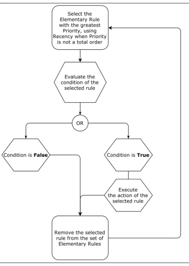
The second part of a BR program interpreter is the execution algorithm. We only consider execution algorithms which include a main loop. The standard pattern followed by an execution algorithm with a main loop is conceptually simple: 1. Select as executable rules all the instances of elementary rules for which the
condition is True, using the current values of the variables
2. Check a preset Halting condition and stop if it is True
3. Use a preset conflict resolution strategy to select a single rule instance from the set of executable rules selected in step 1.
4. Execute the action of the selected executable rule 5. Restart from step 1.
In the rest of this thesis as well as in all commercial BRMS, the default Halting condition in step 2 is True if and only if (iff) there is no executable rule identified in step 1, i.e. if all conditions are False. In some BRMS, the Halting condition can also be True if alternate conditions are fulfilled. However, such alternate Halting conditions can always be replaced by the default one, by embedding the Halting test in the rules’ conditions. Let the Halting condition be H(x), we simply add an extra condition to each BR. Given a BR with condition T (x), we replace it by
¬H(x) ∧ T (x). We can then replace H(x) by the default Halting condition. As a
consequence, we describe no such alternate conditions in this thesis.
The most basic interpreter I0 for a BR program follows this pattern. The conflict resolution strategy it uses in its execution algorithm consists in a preset total order over all possible elementary rules, which lets the interpreter select the greatest elementary rule for that order relation. The order of elementary rules used is defined by the lexicographic order derived from a predefined order on the rules in the rule set to execute and a predefined order on input variables. This is illustrated in Fig. 2.1. In this thesis, we only consider the basic interpreter, as we can use it to simulate any more complicated ones.
The most common conflict resolution strategies combine one or more of the following three elements [137]:
Figure 2.1: Control flow corresponding to the basic interpreter
• Refraction which prevents an elementary rule from being selected by the conflict resolution algorithm after it is executed unless its condition clause has been reset in the meantime.
• Priority which is a partial order on rules, leading of course to a partial order on elementary rules.
• Recency which orders elementary rules in decreasing order of continued va-lidity duration (when elementary rules are created at run time, it is often expressed as increasing order of elementary rule creation time).
These elements can be simulated by the basic interpreter by adding more types, variables or rules, in broad strokes:
• Refraction is simulated with the use of an additional boolean variable (e.g.
needsReset) per rule per variable permutation (i.e. per elementary rule),
an additional test clause and assignment action in each rule, and an ad-ditional rule per rule r (if needsResetx,r = True∧ Tr(α, x) = False then
needsResetx,r ← False).
• Priority results in one additional integer variable p, an additional test clause in each rule (p = πr), an additional action clause in each rule (p← pmax), and two additional rules that come dead last in the predefined order on rules (if
p > 0 then p← p − 1; if p = 0 then Stop). The second of those additional
rules can in turn be transformed into an additional test clause in each rule, as mentioned earlier.
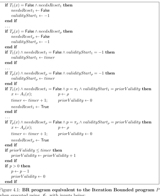
• Recency is the most complicated. A possible simulation could involve an additional integer variable validityStart per elementary rule, an additional integer variable timer, an additional action clause in each rule (timer ←
timer + 1) and a similar setup to the one suggested for priority, using an
integer variable priorV alidity which would this time start at 0 and end at
timer.
The Business Rules transformed and created by those modifications, with any pre-defined order which puts the rules created to increment the p and priorV alidity counters at the very bottom, simulates an interpreter with those conflict resolution elements inI0. We call IS the standard BR interpreter which uses the aforemen-tioned execution loop as well as those three conflict resolution strategy elements. It is illustrated in Fig. 2.2.
Some degenerate execution algorithms do not include a main loop, as many users of BRMS do not require the recursive ability of the standard interpreter.
Figure 2.2: Control flow corresponding to the standard interpreter
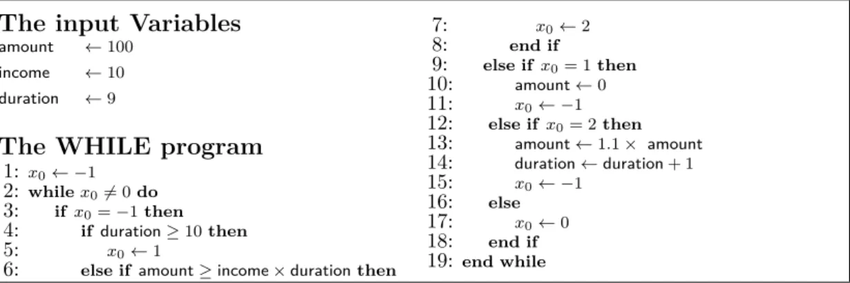
In fact, any BR program in which the BRs have only monotonous actions, in the sense that the actions only affect variables which do not appear in the condition of any BR, can be executed by a simplified non-looping algorithm without changing the output. In particular, any direct translation of a decision tree (in which the leaves do not affect the tested attributes) into BRs can be executed on any input with a single check of each condition. This has led to the appearance of simplified execution modes in BRMS, such as the sequential execution mode in ODM, which uses the algorithm illustrated in Fig. 2.3:
• Take each BR in order, and for each evaluate its condition then execute its action if the condition is True
Another example of such is the “FastPath” algorithm available as an execution mode in ODM, which simply evaluates the BRs’ conditions all at once, then ex-ecutes the actions of each BR r such that Tr = True in an often preset arbitrary order. Such algorithms are popular in some industrial contexts as they simplify the BR engine to the point where the BR program does exactly what the non-programmer thinks it does, instead of doing so most of the time. However, BR languages defined using such algorithms are not as expressive as BR languages which use a main loop, as non-degenerate execution algorithms must evaluate an unbound number of evaluations of BR conditions, which leads to possible non-terminating inputs. In other words, non-looping execution algorithms are degener-ate in the sense that they do not allow for any inference, whether forward-chaining or backwards-chaining.
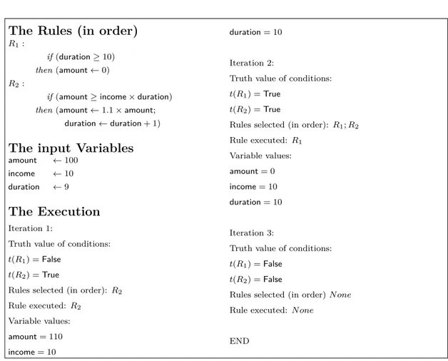
An example of the execution a BR program using the basic interpreter I0 is described in Fig. 2.4, using the toy example of a BR program which takes as input the value amount of a requested loan (including interest), the yearly income of the requester and the duration (in years) of the repayment, then outputs either the original values (if the request is valid), an alternate loan which can be repaid, or an amount of zero if there is no possible repayment plan. This toy example supposes that the compound interest rate is 10% per year.
2.2
Machine Learning (ML)
The problem examined in this thesis, the parametrization of a BR program in light of a statistical objective, can be seen as a ML problem. The main purpose of using ML in our work is to provide an existing framework to examine our problem, as
Figure 2.3: Control flow corresponding to the sequential execution algorithm from ODM
well as use the known results pertaining to the learnability of function classes to prove that it cannot be solved in the general case.
Research linking Production Rules and Machine Learning has recently focused on transforming the product of ML techniques, such as decision trees or associa-tion rules, into executable producassocia-tion rules [124, 102, 11]. Past efforts have also used Production Systems as learning systems themselves, among other works on learning by doing [9, 141]. The ML problem of modifying an existing computer program or complex function to account for new data is sometimes called theory
The Rules (in order)
R1:
if (duration≥ 10) then (amount← 0) R2:
if (amount≥ income × duration) then (amount← 1.1 × amount;
duration← duration + 1)
The input Variables
amount ← 100 income ← 10 duration ← 9
The Execution
Iteration 1:
Truth value of conditions: t(R1) = False
t(R2) = True
Rules selected (in order): R2
Rule executed: R2 Variable values: amount = 110 income = 10 duration = 10 Iteration 2:
Truth value of conditions: t(R1) = True
t(R2) = True
Rules selected (in order): R1; R2
Rule executed: R1 Variable values: amount = 0 income = 10 duration = 10 Iteration 3:
Truth value of conditions: t(R1) = False
t(R2) = False
Rules selected (in order) N one Rule executed: N one
END
Figure 2.4: Example illustrating the execution algorithm: smallest loan payment plan
revision [51]. The theory revision problem restricted to modifying parameters of the existing theory is similar to our problem. An approach to the non-statistical theory revision applied to Business Rules appears in [31], working with CLIPS-R. Answers to the theory revision problem with access to labeled data points (with a known label for each input) appear in [4, 64, 65]. We work on extending work made on this problem to statistical goal learning problems in Production Rules systems, in particular BR systems.
In this section, we first formally express our problem and contrast it to existing ML formulations. We then present some existing results we will use in Chapter 3
pertaining to the learnability of function classes.
2.2.1
Statistical goal learning
One of the challenges of BR systems in the current industry is maintaining the flexibility that has lead to its adoption as the automatic decision management tool of choice by many organizations. While BRMS make it simple to maintain and modify BR programs, they do not offer a way to predict the effect of any modification, nor do they supply a framework for Machine Learning (ML) of BR programs in view of a goal. Business Users must rely on their knowledge of the business process and the goal to implement any modifications to the BRs on their own. In a digitalized world where ML and “big data” are becoming more than buzzwords, this can undermine the agility of BRMS, or at least make it costly and inefficient.
The goals of such modifications can be of a statistical nature, e.g. adjusting the average decision over a given set of inputs. For example, a bank might require that no more than a certain percentage, e.g. 30%, of all requested loans be examined manually, due to human resource concerns. As the number of manually examined loan requests should always be as high as possible, the goal is in fact to have the BR program which determines such things assign 30% of all loan requests to manual examination. Such a requirement could be fulfilled by automatically learning the “right values” of some adjustable parameters in the corresponding BR program. If the output of the BR program is a binary variable using 1 for manual evaluation and 0 for automatic evaluation of a loan request, the learning problem would be to find the values of the parameters which satisfy the statistical goal: “average of all outputs is 0.3”. This could arise as a consequence of exceptional circumstances, e.g. a new legislation, or of natural trend evolution, e.g. the client base changing so that too many or too few loan requests are evaluated automatically.
Such a learning problem is what we henceforth call a statistical goal learning problem, as the goal is not over the output of the system but over the average of that output given a set of inputs. A broader definition of statistical goal learning goes beyond the average, and involves target statistical distributions in the outputs given a certain statistical distribution of inputs. An algorithm for the “narrower” version of the statistical goal learning problem will be discussed in Chapter 4. The broader version will be discussed in Chapter 5.
In the rest of this thesis, we characterize a BR program which must be learned this way by its input, output and parameters. The input is the initial value of the variables when executing the BR program, the output is the final value of the scalar variable chosen as the BR program’s result and the parameters are the elements of the BRs which can be modified by the learning algorithm.
Definition 2.4 (Family of BR program). We call family of BR programs derived
from a BR program the set of functions P (p, .) with values inR, where p ∈ π is a
parameter or vector of parameters of the BRs, such that for any valid input x∈ X
of the BR program, the output of the BR program modified by using the values p in place of predefined elements of BRs x is P (p, x).
Let P (p, .) be a family of BR programs parametrized over p ∈ π ⊆ Rϕ, with input x∈ X ⊆ Rd. Let g∈ R be the desired goal. The “narrower” statistical goal learning problem can then be formalized as:
min p ∥p − p 0∥ Eq∈Q [ f(P (p, q))]− g ≤ ε, (2.2)
where ∥ · ∥ is a given norm, E is the usual notation for the expected value, Q is a training set of inputs and ε is a given tolerance.
(minimizingE(P )−g while constraining p−p0), as corporations will often consider goals more rigidly than changes to the business process, and the value of the objective will speak to them more as a kind of quantification of the changes to be made. The form this quantification takes, from minimizing the variation of each parameter in p to minimizing the number of parameters whose value is modified, depends on the definition of the norm ∥ · ∥. In terms of business modeling rules, this means that we can for example choose to try and change the rules minimally with many rules being changed, or we can try to change a minimal number of rules, even if the change is very big.
ML has many existing approaches and algorithms depending on what is to be learned and how it may be learned [80], the commonality being that ML aims to use training data in order to predict the behavior of other inputs, usually by learning a predictor function. In general, one may divide ML approaches into Supervised Learning and Unsupervised Learning [131], with problems of Semi-Supervised Learning straddling the line. In Semi-Supervised Learning, the training data is labeled, meaning the known data consists of both inputs and outputs of the function we wish to learn. In contrast, Unsupervised Learning only provides inputs, i.e. uses unlabeled training data and assumptions about the outputs (such as the number of classes in classification problems). In Semi-Supervised Learning problems, only some of the data is labeled. Those problems are usually studied as either imperfect Supervised Learning problems or constrained Unsupervised Learning problems.
Our problem lies somewhere between the two main approaches, as we do have information beyond the simple input data: we know both the original output of the BR program and the statistical distribution of the outputs we wish to achieve. The specificity of our problem however is that this information does not take the form of labels over data points, as in Supervised Learning. Instead, the
informa-tion we have is closer to ‘statistical labels’, i.e. labels over data sets instead of data points. Just as in Unsupervised Learning, the relevance of the training data, usually historical data, lies solely in its statistical properties: the specific values are not important, as they are not individually labeled. The information we have about the desired distribution of outputs is also comparable to a (non-standard) assumption about the output made by Unsupervised Learning algorithms. Semi-Supervised Learning problems however are entirely unrelated to ours, since the problem is not one of partial labeling. While both the Supervised and Unsu-pervised approaches have been studied extensively, the UnsuUnsu-pervised Learning approach mostly focuses on classification problems, whether through clustering algorithms such as the k-means algorithm [47] or through association algorithms such as the Apriori algorithm [3]. Furthermore, using an Unsupervised approach would lead to disregarding the information encoded in the existing BR program. Such an approach is more applicable to initial learning of BRs, as some software (like IBM SPSS Modeler [117, 118]) can do in a limited fashion.
Consequently, similarities to our problem are better found among Supervised Learning problems. The traditional Supervised Learning problems are regression, for continuous outputs, and classification, for discrete outputs. The standard su-pervised learning algorithms are summarized by Hastie, Tibshirani and Friedman in [78]. The best known algorithms are Support Vector Machines [120], neural nets [84], logistic regression, naive bayes [106], k-nearest neighbors [67], random forests [104], and decision trees. Those methods, among others, are compared in [79] for the classification problem.
All of these methods consider the “classic” supervised learning problem, of which a generic formulation is the following, with a function f to be learned:
min ˆ f∈F (f (x)ˆ − y(x)) x∈X (2.3)