DEVELOPMENT OF A METHODOLOGY TO ASSESS
FUTURE TRENDS IN LOW FLOWS AT THE WATERSHED SCALEUSING SOLELY CLIMATE DATA
Étienne Foulon1, Alain N. Rousseau1,Patrick Gagnon2
1 INRS-ETE/Institut National de la Recherche Scientifique—Eau Terre Environnement, 490 rue de la Couronne, Quebec City, Quebec G1K 9A9, Canada
2 Agriculture and Agri-Food Canada, 2560 Boulevard Hochelaga, Quebec City, Quebec, G1V 2J3, Canada
*Revised Manuscript with no changes marked Click here to view linked References
A
BSTRACT
1Low flow conditions are governed by short-to-medium term weather conditions or long term 2
climate conditions. This prompts the question: given climate scenarios, is it possible to 3
assess future extreme low flow conditions from climate data indices (CDIs)? Or should we 4
rely on the conventional approach of using outputs of climate models as inputs to a 5
hydrological model? Several CDIs were computed using 42 climate scenarios over the years 6
1961 to 2100 for two watersheds located in Québec, Canada. The relationship between the 7
CDIs and hydrological data indices (HDIs; 7- and 30-day low flows for two hydrological 8
seasons) were examined through correlation analysis to identify the indices governing low 9
flows. Results of the Mann-Kendall test, with a modification for autocorrelated data, clearly 10
identified trends. A partial correlation analysis allowed attributing the observed trends in HDIs 11
to trends in specific CDIs. Furthermore, results showed that, even during the spatial 12
validation process, the methodological framework was able to assess trends in low flow 13
series from: (i) trends in the effective drought index (EDI) computed from rainfall plus 14
snowmelt minus PET amounts over ten to twelve months of the hydrological snow cover 15
season or (ii) the cumulative difference between rainfall and potential evapotranspiration over 16
five months of the snow free season. For 80% of the climate scenarios, trends in HDIs were 17
successfully attributed to trends in CDIs. Overall, this paper introduces an efficient 18
methodological framework to assess future trends in low flows given climate scenarios. The 19
outcome may prove useful to municipalities concerned with source water management under 20
changing climate conditions. 21
22
Keywords:
23
effective drought index; 7-day low flow; 30-day low flow; HYDROTEL; trends; climate model 24
1. Introduction
25A persistent lack of precipitation (meteorological drought) can affect soil moisture 26
(agricultural drought) as well as groundwater and surface flows (Tallaksen and Van Lanen, 27
2004; Mishra and Singh, 2010), resulting in a hydrological drought and low flows. The 28
frequency of short hydrological droughts is likely to increase due to climate change, and thus, 29
it is expected to have a strong impact at various spatial scales (i.e., local, regional, and 30
global scales) (Jiménez Cisneros et al., 2014). Given this context, studies around the world 31
have looked at low flow hydrological indices (HDIs) and associated temporal variability from 32
observed series of data (Zhang et al., 2001; Svensson et al., 2005; Ehsanzadeh and 33
Adamowski, 2007; Khaliq et al., 2009; Fiala et al., 2010; Yang et al., 2010; Masih et al.,
34
2011). But, as Smakhtin (2001) clearly demonstrated in his review, a clear understanding of 35
low flow hydrology can help resource specialists manage, for example, municipal water 36
supply, water allocations (i.e., for irrigation and industrial activities), river navigation, 37
recreation, and wildlife conservation. Observed trends in low flows need to be explained and 38
attributed to their underlying causes. Worldwide, there are few related studies and most of 39
them linked trends in monthly or yearly flows to cumulative precipitation or temperature at the 40
same temporal scale (Mavrommatis and Voudouris, 2007; Khattak et al., 2011; Ling et al., 41
2013; Huang et al., 2014; Li et al., 2014; Kour et al., 2016). In Canada and the USA, trends 42
in low flow HDIs have actually been linked to specific climate data indices (CDIs) computed 43
from cumulative rainfall, precipitation or degree-days over the course of one month up to a 44
year (Yang et al., 2002; Burn et al., 2004a; Burn et al., 2004b; Cunderlik and Burn, 2004; 45
Hodgkins et al., 2005; Abdul Aziz and Burn, 2006; Novotny and Stefan, 2007; Burn, 2008;
46
Assani et al., 2011; Masih et al., 2011; Assani et al., 2012). For example, Assani et al. (2011)
47
linked, for the south-east region of the St. Lawrence River watershed, an increase in summer 48
7-day low flows to an increase in summer precipitation. In the Zagros Mountains of Iran near 49
Ghore Baghestan, Masih et al. (2011) linked a decline of the low flow conditions (1 and 7 50
days minima) to a decline in precipitation during April and May. It is noteworthy that, links 51
between HDIs and large-scale climate indices such as NAO or ENSO are beyond of the 52
scope of this study. 53
All the aforementioned studies that locally linked HDIs to CDIs have relied on a statistical 54
framework. As such, they required series of flow data to predict how changing climate 55
conditions would affect hydrology at the watershed scale. However, it is possible to use a 56
hydroclimatological modeling framework to anticipate this effect; combining a hydrological 57
model and climate scenarios (Cunderlik and Simonovic, 2005; Cloke et al., 2010; CEHQ, 58
2013b, 2015). This approach remains challenging and cannot be readily applied by any 59
water organization because of the required expertise. Moreover, it combines uncertainties 60
associated with climate simulations, bias correction as well as hydrological modeling (Dobler 61
et al., 2012; Teng et al., 2012) and the specific challenges associated with the modeling of
62
low flows (Smakhtin, 2001; Staudinger et al., 2011). 63
To the best of the authors’ knowledge, no study has yet investigated the potential of directly 64
assessing HDI trends given climate scenarios. To fill this gap, this paper combines the two 65
aforementioned frameworks in creating a statistical framework that captures past statistical 66
relationships between CDIs and HDIs and apply the latter relationships into the future. 67
Demonstrating the effectiveness of this novel approach required computing HDIs using a 68
hydrological model in order to show that it worked before actually bypassing this modeling 69
step. To ensure that the drought-inducing mechanisms were well covered and that the 70
method was as universal as possible, the proposed methodology relied on a broad set of 71
complementary CDIs computed for time steps varying from one day to a year using daily 72
precipitation and minimum and maximum temperatures. 73
This paper is organized in four sections: (i) Material and methods, (ii) Results, (iii) 74
Discussion, and (iv) Conclusions. The proposed methodology was developed using a case 75
study in Québec, Canada for which: (i) future climate was built from the IPCC greenhouse 76
gas emissions scenario SRES-A2 (Nakicenovic et al., 2000; Environnement Canada, 2010) 77
for the 2001-2100 period, (ii) uncertainty of the climate change signal was addressed through 78
the use of 42 climate simulations, and (iii) future flows were simulated using a distributed 79
hydrological model. 80
2. Materials and methods
81The organization and mapping of the Materials and methods and Results sections are 82
introduced in Figure 1. Throughout the paper, and in accordance with CEHQ (2013a); IPCC 83
(2013), “simulation” or “climate simulation” refers to the raw climate model outputs. 84
“Scenario” or “climate scenario” refers to a post-processed simulation, which is a simulation 85
for which a series of specific choices have been made (study region and period, spatial and 86
temporal resolutions, bias-correction method). White boxes present how the climate 87
scenarios were obtained from 42 different bias-corrected climate simulations. Grey boxes 88
introduce the methodological framework proposed in this paper. It required computing CDIs 89
from climate data extracted from the aforementioned climate scenarios and HDIs from 90
simulated streamflows using a calibrated hydrological model. Afterwards, the statistical 91
relationships between CDIs and HDIs were assessed through a correlation analysis followed 92
by trend detection and partial correlation analyses. Black boxes refer to the results of the 93
application of the methodological framework to a case study in Québec, Canada described in 94
the next subsection. 95
Figure 1: Detailed schematic of the methodological framework and mapping of the sections of this paper.
96
White boxes stand for the computing of climate scenarios; grey boxes refer to the Material and methods
97
section; and the black boxes refer to the Results section.
98
2.1 Case study
99
2.1.1 Study area
100Recent studies have predicted a decrease in summer flows for southern Québec, Canada 101
(Minville et al., 2008; CEHQ, 2013b, 2015). More especially, the Yamaska River is
102
characterized by very low flow conditions during summer, as indicated by flow records 103
(Trudel et al., 2016). For this study, the proposed methodology was developed using two
watersheds (Figure 2) of the St. Lawrence Lowlands (Québec, Canada): (i) Bécancour and 105
(ii) Yamaska. They were chosen for their geophysiographical proximity and to demonstrate 106
the application potential on: (i) an unregulated watershed and (ii) a watershed with partially 107
regulated flows. This provided a framework well suited for comparing results and getting 108
insights into the possibility to export the captured statistical relationships from one watershed 109
to another. 110
Figure 2: Location of the study watersheds in: (a) the province of Québec and (b) the St. Lawrence River
111
lowlands
112
The Bécancour River drains a 2,620-km² watershed (Labbé et al., 2011). More than half of 113
the landscape is forested and interspersed with agriculture areas (30%), while urban area 114
represents 5.2% of the watershed with a population density of 25 people per km². The 115
population of the watershed is approximately 64,000 inhabitants and is concentrated in 116
Thetford Mines (25,790 inhabitants in 2011) and Plessiville (6,688 in 2011). Low flows 117
typically happen between July and September and around February while the spring flood 118
starts in March and peak flow is often reached in April. This matches a transient snow regime 119
(mixed rain and snow) which entails spring high flows and summer and winter low flows 120
(Morin and Boulanger, 2005).
121
The Yamaska River drains a 4,784-km² watershed (Labbé et al., 2011). The watershed is 122
mostly agricultural (52.4%) and forested (42.8%) while the urban area is comparable to the 123
Bécancour watershed (3.1%). There are 250,000 people in the watershed (52 people per 124
km²) mostly concentrated in Granby (66,000 inhabitants in 2014), Saint-Hyacinthe (54,500 125
inhabitants in 2014) and Cowansville (13,000 inhabitants in 2015). Low flows typically occur 126
at the same time as those of the Bécancour watershed. 127
St. Hyacinthe and Rivière Noire, two towns located in the Yamaska watershed, have had to 128
deal with a critical water availability problem one year out of five (based on the 1971-2000 129
period). For the 2041-2070 time period, Côté et al. (2013) indicated that in all likelihood it 130
would be the case one year out of two. Since water shortages are likely to occur in other 131
towns throughout Quebec and elsewhere in the world, therefore, robust tools that do not 132
require hydrological modeling and could be readily used by any water utility organization are 133
needed. 134
2.1.2 Hydrological seasons
135Temporal changes in the hydrology of a watershed can be accounted for through the 136
definition of “hydrologic seasons”; dividing the year into distinct time periods of similar 137
conditions (Curtis, 2006). Two hydrological seasons were defined according to climate 138
variability and signal characterizing the length of the study period (1961-2100): (i) a snow-139
free (SF) season, and (ii) a snow-cover (SC) season. They were defined in terms of snow 140
water equivalent (SWE) according to the following rules. SC season starts on the first day d 141
beyond August that satisfies the following condition: 142
Eq 1 143
Namely, the SWE needs to be greater than 10 mm and increasing for at least eight 144
consecutive days for the SC season to begin. The SC season ends on the first day d that 145
meets the following condition: 146
Eq 2 147
Namely, the SWE is less than 10 mm and decreasing for at least eight consecutive days. 148
The SF season starts on day d+1. If the SF season does not end before the calendar year, it 149
continues onto the next one until conditions are met for the SC season to start, meaning that 150
some years, especially in the future, may not have a SC season. The SWE threshold value 151
(10 mm) and the number of consecutive days (8 days) were selected after sensitivity tests 152
(included in supporting material 1). In more mountainous regions such as the Alps or the 153
Rocky Mountains, these two parameters would need to be calibrated to reflect local 154
hydrological processes and to differentiate low flows during the ice cover period from the 155
open water period. Rousseau et al. (2014) and Klein et al. (2016) also chose a 10-mm 156
threshold to assess whether a precipitation event was occurring in summer/fall (SWE<10mm) 157
or in spring (SWE>10mm). 158
2.2 Climate simulations
159
To investigate the effect of global warming on low flows, two IPCC greenhouse gas 160
emissions scenarios were used: “observation of the 20th century” for the 1961-2000 period 161
and SRES-A2 (Nakicenovic et al., 2000; Environnement Canada, 2010) for the 2001-2100 162
period. The A2 emission scenario was used because observations of CO2 atmospheric 163
global emissions are at the high end of the plausible IPCC SRES emissions projections 164
(Raupach et al., 2007; Rousseau et al., 2014). The selected simulations represented 42 of
165
the 87 original simulations from a climate ensemble called (cQ)² and produced by the 166
Ouranos consortium (Guay et al., 2015). They consisted of simulations from the World 167
Climate Research Programme phase 3 (CMIP3) (Meehl et al., 2007a), the North American 168
Regional Climate Change Assessment Program (NARCCAP) (Mearns et al., 2012), and the 169
Canadian Regional Climate Model (CRCM) (Music and Caya, 2007; de Elia and Côté, 2010; 170
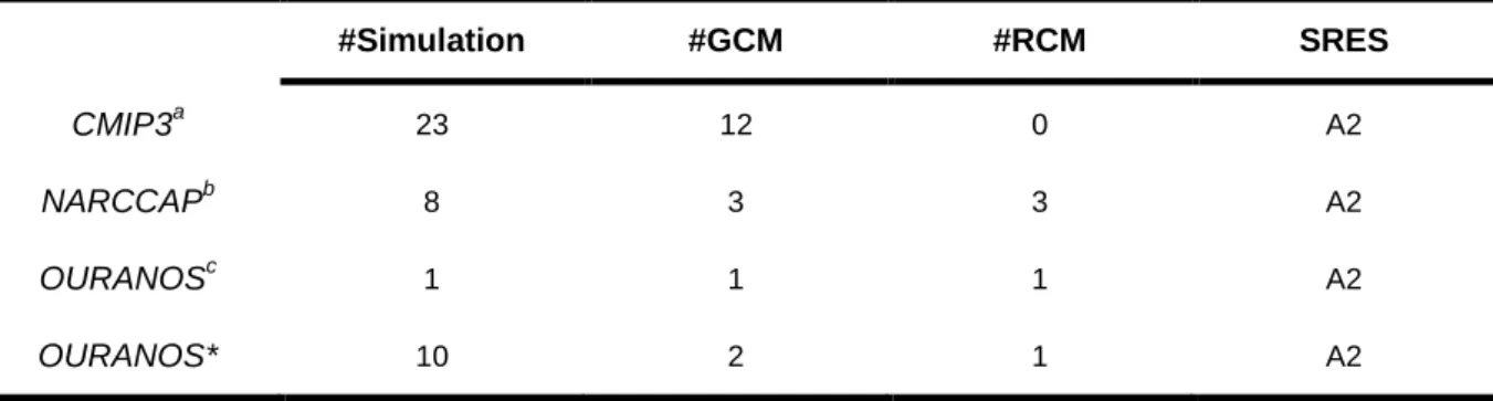
Paquin, 2010) operational runs supplied by Ouranos. The 42 simulations introduced in Table
171
1 are based on 14 global climate model (GCM) runs with different initial conditions (one to 172
five members) and four different regional climate models (RCMs). They were selected to 173
avoid dependencies between models while covering all sources of climate uncertainty apart 174
from the emissions scenario uncertainty (Hawkins and Sutton, 2011), which is discussed 175
later on. 176
Table 1: Description of the 42 climate simulations extracted from the (cQ)² project and generated by 177 CRCM version 4 178 #Simulation #GCM #RCM SRES CMIP3a 23 12 0 A2 NARCCAPb 8 3 3 A2 OURANOSc 1 1 1 A2 OURANOS* 10 2 1 A2 a
GCM used: BCCR_BCM2.0; CSIRO_MK3.0; CSIRO_MK3.5; CCCMA_CGCM3.1; GFDL_CM2.0;
179
CNRM_CM3; IPSL_CM4; INGV_ECHAM4; ECHAM5; MIUB_ECHO_G; MIROC3.2_MEDRES;
180
MRI_CGCM2.3.2a
181 b
GCM used : CCSM; HADCM3; CCCMA_CGCM3.1; GFDL_CM2.0. RCM used: HRM3; RCM3; WRFG
182 c
GCM used:CNRM_CM3. RCM used: CRCM4
183
*Simulations generated by the CRCM4 that cover 1961 to 2100 continuously (GCM used:
184
CCCMA_CGCM3.1; ECHAM5)
185
Simulation data were corrected using the daily translation method (Mpelasoka and Chiew, 186
2009) which is a quantile-quantile mapping technique removing the bias of climate model 187
outputs. The temperature correction is additive while the correction for precipitation is 188
multiplicative. The reader is referred to the following publications for more details (Wood et 189
al., 2004; Lopez et al., 2009; Mpelasoka and Chiew, 2009; Guay et al., 2015). This method
190
conserves the different characteristics and dynamics of each individual climate model. Each 191
climate simulation has a temporal sequence of meteorological events which are different 192
between member simulations. The post-processing method assumes the biases to be of 193
equal magnitude in the future and reference periods; that is the relationship between 194
simulated and observed data is still applicable in the future (Huard, 2010). The reference 195
period 1961-2000 and observed precipitation data came from a 10-km grid covering southern 196
Canada, that is south of 60°N (Hutchinson et al., 2009) averaged on the RCM or GCM grid 197
before application of the bias correction methodology. Finally, besides the ten simulations 198
supplied by Ouranos covering the 1961-2100 period continuously, other simulations (32) 199
were available for two temporal horizons: (i) the past horizon (1971-2000) and (ii) future 200
horizon (2041-2070). As a consequence, the following methods and results are presented for 201
two temporal horizons. 202
2.3 Climate data indices – CDIs
203
Daily precipitation and minimum and maximum temperatures at two meters of elevation were 204
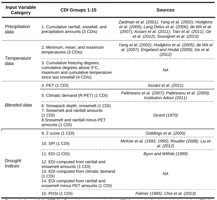
retrieved, from the climate scenarios (Figure 1). Table 2 introduces the CDIs used in this 205
study; they were taken from the literature based on their widespread use, data requirements, 206
and potential to corroborate (assessed through linear correlation coefficients) with low flow 207
HDIs. The CDIs are divided into four categories with respect to the type of input data needed 208
for their computation, that is computed from: (i) precipitation data, (ii) temperature data, (iii) 209
blended data (both precipitation and temperature), and (iv) drought indices formulas. Other 210
CDIs could be included if other HDIs were to be studied, illustrating the flexibility of the 211
methodology being developed in this paper. The CDIs used are computed starting on the day 212
of occurrence of each individual HDI and continuing backward in time, providing a framework 213
for future work on forecasting extreme flow conditions. 214
Table 2 : Overview of the CDI groups used
215
Input Variable
Category CDI Groups 1-15 Sources
Precipitation data
1. Cumulative rainfall, snowfall, and precipitation amounts (3 CDIs)
Zaidman et al. (2001); Yang et al. (2002); Hodgkins et al. (2005); Lang Delus et al. (2006); de Wit et al.
(2007); Assani et al. (2011); Tian et al. (2011); Ge et al. (2012); Souvignet et al. (2013)
Temperature data
2. Minimum, mean, and maximum temperatures (3 CDIs)
Yang et al. (2002); Hodgkins et al. (2005); de Wit et al. (2007); Engeland and Hisdal (2009); Ge et al.
(2012)
3. Cumulative freezing degrees, cumulative degrees above 0°C, maximum and cumulative temperature since last snowfall (4 CDIs)
NA
Blended data
4. PET (1 CDI) Assani et al. (2011)
5. Climatic demand (R-PET) (1 CDI) Paltineanu et al. (2007); Paltineanu et al. (2009);
Institution Adour (2011)
6. Snowpack depth, snowmelt (1 CDI) 7. Snowmelt and rainfall amounts (1 CDI)
8.Snowmelt and rainfall minus PET amounts (1 CDI)
Girard (1970)
Drought Indices
9. Z score (1 CDI) Giddings et al. (2005)
10. SPI (1 CDI) McKee et al. (1993, 1995); Roudier (2008); Liu et
al. (2012)
11. EDI (1 CDI) Byun and Wilhite (1999)
12. EDI computed from rainfall and snowmelt amounts (1 CDI)
13. EDI computed from climatic demand (1 CDI)
14. EDI computed from rainfall and snowmelt minus PET amounts (1 CDI)
NA
15. PDSI (1 CDI) Palmer (1965); Choi et al. (2013)
R stands for rainfall, PET for Potential evapotranspiration, SPI for standardized precipitation index, EDI for
216
effective drought index, PDSI for Palmer drought severity index.
217
The PDSI and SPI are two normalized drought indices that allow detection of dry as well wet 218
periods. The PDSI is a cumulative index, computed on a monthly basis (Heddinghaus and 219
Sabol, 1991) and has been linked to monthly flows (r=0.83, p<0.01) by Choi et al. (2013).
220
The SPI assesses short term water supply deficit or surplus as well as long-term 221
groundwater supplies. It is computed as a rainfall departure (Wilhite and Glantz, 1985; Liu et 222
al., 2012) from any timescale. The climatic demand computes the difference between
223
precipitation and PET (thus in the blended data type). In Romania, it has been combined to 224
the SPI to identify water quantity issues (Paltineanu et al., 2007). The EDI is a drought 225
recursive index based on the effective precipitation concept (Byun and Wilhite, 1999). It 226
takes into account antecedent rainfall conditions and is computed on a daily basis while 227
accounting for past (from 15 to 365 days) rainfall amounts with a decreasing weight. 228
Because it does not consider any location or climate characteristics, it can be used anywhere 229
(Roudier, 2008; Akthari et al., 2009; Deo et al., 2016).
230
Except for the Z score which is conceptually equivalent to the SPI (standardized anomaly of 231
the precipitation), the SPI, and the PDSI that were computed on a monthly basis, the CDIs 232
introduced in Table 2 were all computed for 18 time steps starting on the day of occurrence 233
of each individual HDI and going backward in time (one to six days, one to three weeks, one 234
to six months, eight, ten and twelve months). 235
2.4 Hydrological model
236
In this paper, HYDROTEL is the hydrological model calibrated from observed data and used 237
to generate the series of past and future HDIs (Figure 1). It is a process-based, continuous, 238
semi-distributed hydrological model (Fortin et al., 2001; Turcotte et al., 2003; Turcotte et al., 239
2007; Bouda et al., 2012; Bouda et al., 2014), and currently used for inflow forecasting by 240
Hydro-Quebec, Quebec’s major power utility, and the Quebec Hydrological Expertise Centre 241
(CEHQ). It was designed to use available remote sensing and GIS data at either a 3-h or a 242
daily time step. It is based on the spatial segmentation of a watershed into relatively 243
homogeneous hydrological units (RHHUs, elementary subwatersheds or hillslopes as 244
desired) and interconnected river segments (RSs) draining the aforementioned units. A semi-245
automatic, GIS-based framework called PHYSITEL (Turcotte et al., 2001; Rousseau et al., 246
2011; Noël et al., 2014) allows easy watershed segmentation and parameterization of the 247
hydrological objects (RHHUs and RSs). The model is composed of six computational 248
modules, which run in successive steps. Each module simulates a specific hydrological 249
process and the reader is referred to Fortin et al. (2001) and Turcotte et al. (2007) for more 250
details on these aspects of HYDROTEL. 251
2.4.1 Calibration and validation
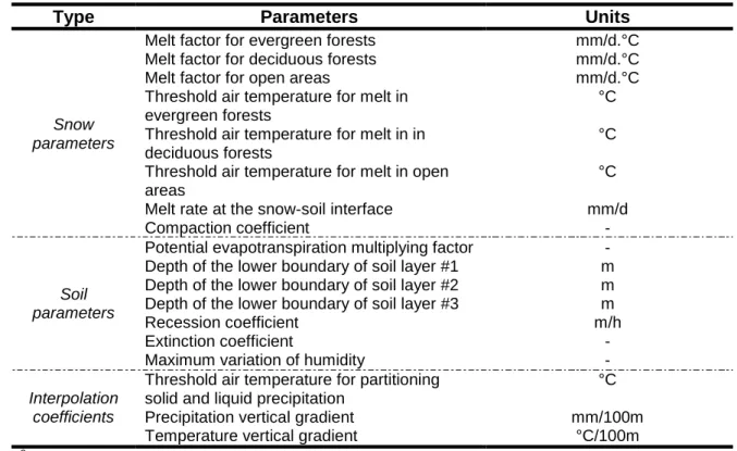
252The main calibration parameters of HYDROTEL can be grouped (Table 3) into snow 253
parameters, soil parameters, and interpolation coefficients for temperature and precipitation. 254
Interpolation is computed as the average of the three nearest meteorological stations 255
weighted by the square of the inverse distances between a RHHU and the stations 256
(Reciprocal-Distance-Squared method). 257
Table 3: HYDROTEL key parameters
258
Type Parameters Units
Snow parameters
Melt factor for evergreen forests mm/d.°C
Melt factor for deciduous forests mm/d.°C
Melt factor for open areas mm/d.°C
Threshold air temperature for melt in evergreen forests
°C Threshold air temperature for melt in in
deciduous forests
°C Threshold air temperature for melt in open
areas
°C
Melt rate at the snow-soil interface mm/d
Compaction coefficient -
Soil parameters
Potential evapotranspiration multiplying factor -
Depth of the lower boundary of soil layer #1 m
Depth of the lower boundary of soil layer #2 m
Depth of the lower boundary of soil layer #3 m
Recession coefficient m/h
Extinction coefficient -
Maximum variation of humidity -
Interpolation coefficients
Threshold air temperature for partitioning solid and liquid precipitation
°C
Precipitation vertical gradient mm/100m
Temperature vertical gradient °C/100m
a
For a complete description of snow parameters, the reader is referred to (Turcotte et al., 2007)
259 b
For a complete description of soil parameters, the reader is referred to (Fortin et al., 2001)
260
Using the methodology introduced by Turcotte et al. (2003), manual calibration and validation 261
of HYDROTEL was performed over five-year-periods according to available observed climate 262
data provided by the CEHQ for each subwatershed over the 1990-2010 period. As reported 263
by Bouda et al. (2014), when compared with an automatic calibration, the structured, trial-264
and-error, procedure proposed by Turcotte et al. (2003) can achieve very similar 265
performances. Indeed, Bouda et al. (2014) have shown that automatic calibration could 266
provide a marginal improvement over manual calibration (less than 4.2% in terms of Nash-267
Sutcliff Efficiency, NSE). This manual calibration used both NSE and RMSE (m3/s) as 268
objective functions. The modeling performance for low flows was assessed using the Nash-269
log (NSE computed from log transformed flows) objective function which is acknowledged as 270
the best objective function for low flow modeling (Krause et al., 2005). In each case, a one-271
year spin up was used to minimize initialization errors. Observed climate data were 272
computed on a grid (a 28- and 52-point grid for the Bécancour and Yamaska watersheds, 273
respectively) by isotropic kriging following the method described in Poirier et al. (2012) using 274
data collected through the Climate Surveillance Program of the minsitère du Développement 275
durable, de l’Environnement et de la Lutte contre les changements climatiques (MDDELCC).
276
Flow data were extracted from the CEHQ data base (CEHQ, 2012) that includes around 230 277
hydrometric stations throughout Quebec. 278
The Bécancour and Yamaska watersheds were respectively divided into 1813 and 1299 279
hillslopes a.k.a. RHHUs with mean areas of 143 ha and 369 ha and 736 and 513 river 280
segments with mean lengths of 1885 and 3475 m (excluding lakes), defining three regions of 281
interest for parametrization. These regions were used to define local parameter sets of 282
consistent values for the calibration of HYDROTEL. The discretization of both watersheds 283
provided a good representation of the spatial heterogeneity of the landscape while allowing 284
for a reasonable computational time. Three specific river segments and hydrological stations 285
(see Figure 3) were selected for the calibration and validation of each watershed. 286
Figure 3: (a) Bécancour and (b) Yamaska parametrization regions and hydrological stations used for the
287
calibration and validation of HYDROTEL. Red, green, and blue colors stand for upstream, median, and
288
downstream subwatersheds, repectively. # indicates the gauging stations reference number.
289
Data from these stations (#24003, #24014, #24007, and #30302, #30304, #30345 for 290
Bécancour and Yamaska, respectively) were deemed suitable for this study because they 291
are all validated (except for the current year), readily available, and used in hydrological and 292
hydroclimatic impact studies (CEHQ, 2013b; Rousseau et al., 2013; Rousseau et al., 2014; 293
CEHQ, 2015; Fossey and Rousseau, 2016a; Klein et al., 2016; Trudel et al., 2016).
294
Measured flows on the Bécancour watershed are natural while they are partly regulated on 295
the Yamaska watershed. The impact of this regulation will be discussed later on. 296
2.4.2 Computation of the hydrological data indices - HDIs
297The HDIs considered in this paper are the seasonal 7dQmin and 30dQmin, which refer to the 298
seasonal minimum of the 7 and 30 consecutive-day moving average flow, respectively. 299
These HDIs were selected because the MDDELCC uses Q2-7 (2-year annual minimum of the 300
7 consecutive-day average flow) to assess whether water can be abstracted from a specific 301
source (MDDELCC, 2015). Also, the MDDEP uses the Q10-7, or Q2-7, to evaluate the 302
exceedance of water quality criteria for the assessment of pollutant discharge permits 303
(MDDEP, 2007).
304
Once calibrated, the semi-distributed hydrological model HYDROTEL was used to generate 305
past and future seasonal HDIs (for each of the 42 selected climate scenarios) as shown in 306
Figure 1, with the parameter values computed during the calibration/validation process. 307
Indeed, we assumed a similar quality of model responses to future conditions as for the bias 308
correction method for climate models. Precipitation and minimum and maximum 309
temperatures came from the climate scenarios. They were extracted from the nearest ten 310
grid-points of the watershed boundaries before using a Thiessen polygon routine to compute 311
values for each RHHU. 312
To further characterize the capacity of HYDROTEL to simulate flows inducing the observed 313
HDIs, the latter were plotted against HDIs calculated using the calibration/validation dataset. 314
The HDIs computed using the 42 climate scenarios were used to assess the capacity of 315
these selected scenarios to encompass observed values. 316
2.5 Assessing HDIs from CDIs
317
2.5.1 Conditions governing low flows – Correlation analysis
318Pearson as well as Spearman correlation coefficients were calculated to assess the 319
relationships between the four series of seasonal HDIs (7dQmin and 30dQmin for the SC and SF 320
seasons) and the associated CDIs (Table 2). For this study, the post-processing method is 321
based on the following assumptions: (i) the relationships between simulated and observed 322
data for the past-period (1971-2000) will still be applicable in the future (2041-2070); and (ii) 323
the calibrated parameter values are valid over the future time horizon as well. For sake of 324
consistency, a similar assumption was made regarding the relationship between HDIs and 325
CDIs, but verified through what can be seen as a calibration and validation phase of the 326
correlation analysis as is done for hydrological models. The Wilcoxon rank-sum test (Mann 327
and Whitney, 1947) was applied to test whether median correlations between HDIs and CDIs
328
were statistically different between past and future temporal horizons. The validity of these 329
assumptions from the perspective of climate conditions as well as land use and land cover is 330
examined in details in the discussion section of this paper. 331
In short, for each one of the 15 CDI groups introduced in Table 2 and each of the 42 climate 332
scenarios, correlation coefficients were computed individually for each HDI and each season. 333
Then, the best median correlations (maximum absolute median value of the correlation 334
coefficients) for the four CDI categories introduced in Table 1 were identified along with the 335
frequency at which they occurred. Afterwards, the statistical relationships were validated over 336
the future temporal horizon. To account for the fact that many CDIs were tested against each 337
HDI and that correlations could be due to chance, a bootstrap resampling method based on 338
Monte Carlo simulations was applied (Livezey and Chen, 1983) to every CDI-HDI couples as 339
follows: 340
(i) A year was randomly selected from the temporal horizon of interest (past or 341
future). 342
(ii) The paired value (CDI-HDI) for the selected year was added to the resampled 343
data set. 344
(iii) Steps (i) and (ii) were repeated until the resampled data set had the required 345
number of years of data. The required number was set equal to the number of 346
years in the initial data set. 347
(iv) The correlation computation was applied to resampled data set and the result was 348
saved. 349
Steps (i) to (iv) were repeated 1000 times, resulting in a distribution of the correlation 350
coefficients computed from the 1000 resampled data set. The distribution allowed for the 351
determination of the confidence interval (CI) of the correlation coefficient computed from the 352
initial set of data (typically 90 or 95% CI). If the CI minimum was greater than 0, the 353
correlation was then statistically significant. 354
2.5.2 HDI trends and governing drivers
– trend detection and partial correlation
355analysis
356Long term linear trends were analyzed using the non-parametric rank-based Mann-Kendall 357
test (Kendall, 1938; Mann, 1945; Kendall, 1975; Gilbert, 1987) for the four series of HDIs and 358
the associated CDIs obtained through the correlation analysis. The Mann-Kendall (MK) test 359
has been widely used to detect a trend in hydroclimatic time series (Lettenmaier et al., 1994; 360
Lins and Slack, 1999; Douglas et al., 2000; Zhang et al., 2000; Zhang et al., 2001; Yue and
361
Wang, 2002; Novotny and Stefan, 2007; Li et al., 2009). The test is based on the null
362
hypothesis that a sample of data is independent and identically distributed. The alternate 363
hypothesis is that a trend exists in the data. To get more details about this test, the reader is 364
referred to the previous references and especially that of Novotny and Stefan (2007). In the 365
presence of serial correlation or autocorrelation, the assumption of serial independence is 366
violated. The existence of positive serial correlation increases the probability that the MK test 367
detects a trend when none exists (von Storch, 1999), whereas a negative autocorrelation 368
makes it too difficult to find a significant trend (Hamed and RamachandraRao, 1998; Yue and 369
Wang, 2002).The MK test can be modified to obtain the true variance of the MK correlation
370
under the autocorrelation structure displayed by the data (Hamed and RamachandraRao, 371
1998). Tests were conducted for each series of HDIs and CDIs as well as both temporal 372
horizons using the modified MK test to account for autocorrelation. 373
Partial correlations were calculated between each HDI and associated CDIs while controlling 374
for the time step variable. This allowed for the identification of the correlation between 375
variables independent of any common temporal trend signal and for the attribution of the 376
observed trends in HDIs to trends in CDIs (Burn et al., 2004a; Burn, 2008). As for the 377
correlation analysis described in the previous sub-section, trends, especially when they are 378
analyzed for the same CDI-HDI couple for 42 different climate scenarios can be due to 379
chance. Livezey and Chen (1983) indicated the need to consider field-significance of the 380
outcomes of a set of statistical tests. It accounts for the observed cross-correlation in the 381
data for a collection of locations (which in our case was a collection of temporality or climate 382
scenarios) and allows for the determination of the percentage of tests that are expected to 383
show a trend, at a local given significance level, purely by chance. The bootstrap resampling 384
method based on Monte Carlo simulations was thus applied for each scenario following the 385
steps described in the previous subsection except for the fourth step that became: 386
(iv) The Mann-Kendall test was applied to the data from each scenario in the 387
resampled data set and the percentage of results that were significant at the α 388
significance level was determined; α being the local significance level (typically 5 389
or 10%) 390
Steps (i) to (iv) were repeated 1000 times resulting in a distribution of the percentage of 391
results that were significant at the α level. From this distribution, the value that was exceeded 392
β% of the time (typically 5 or 10%) was selected as the critical value. β is referred to as the 393
global significance level. This method was similarly applied in Burn and Hag Elnur (2002); 394
Burn et al. (2004b) and discussed in details in Renard et al. (2008).
395
3. Results
3963.1 Hydrological model
397
This subsection illustrates using the calibration and validation results the capacity of the 398
model to: (i) represent flows in general and low flows in particular and (ii) produce a 399
distribution of HDIs that includes at best the observed values. Presentation of climate data 400
characteristics was beyond the scope of this paper; as such it can be found in supporting 401
material 2. 402
3.1.1 Calibration and validation results
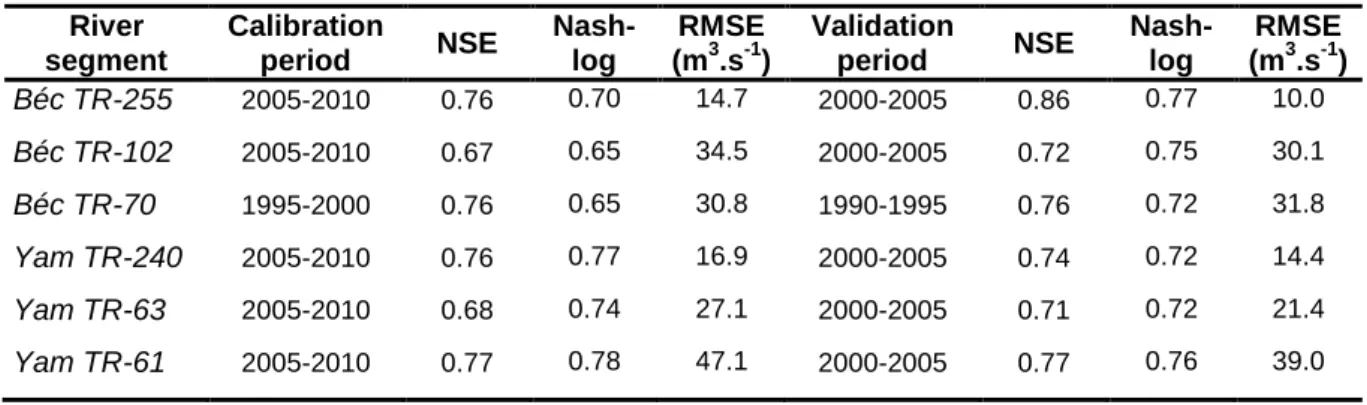
403Model performances for calibration and validation periods of the two study watersheds are 404
given in Table 4. For each river segment, according to the hydrologic model performance 405
rating of Moriasi et al. (2007), the results provide a “good fit” (NSE>0.65) between observed 406
and simulated flows and even a “very good fit” for most of the results (NSE>0.75). Nash-log 407
values vouch for the good representation of low flows with values ranging from 0.65 to 0.70 408
and 0.74 to 0.78 for the calibration period for the Bécancour and Yamaska watersheds, 409
respectively. There is no clear decline in performances between the calibration and validation 410
periods, most even increase between the two periods. This validates the choice of calibration 411
parameters as highlighted in Beven (2006). More especially, Nash-log values are larger for 412
the validation period and range from 0.72 to 0.77 and from 0.72 to 0.76 for the Bécancour 413
and Yamaska watersheds, respectively. 414
Table 4: Model performance for the calibration and validation periods
415 River segment Calibration period NSE Nash-log RMSE (m3.s-1) Validation period NSE Nash-log RMSE (m3.s-1) Béc TR-255 2005-2010 0.76 0.70 14.7 2000-2005 0.86 0.77 10.0 Béc TR-102 2005-2010 0.67 0.65 34.5 2000-2005 0.72 0.75 30.1 Béc TR-70 1995-2000 0.76 0.65 30.8 1990-1995 0.76 0.72 31.8 Yam TR-240 2005-2010 0.76 0.77 16.9 2000-2005 0.74 0.72 14.4 Yam TR-63 2005-2010 0.68 0.74 27.1 2000-2005 0.71 0.72 21.4 Yam TR-61 2005-2010 0.77 0.78 47.1 2000-2005 0.77 0.76 39.0 416
3.1.2 Computation of the HDIs
417The capacity of HYDROTEL to correctly reproduce the HDIs was assessed for the river 418
segments with observed values closest to the outlet of the study watersheds that is TR-70 419
and TR-61 for the Bécancour and Yamaska watersheds, respectively. Figure 4 and Figure 5 420
introduce the boxplots of the seasonal HDIs computed using the results of the hydrological 421
modeling of the climate scenarios (post-processed simulations) for the Bécancour and 422
Yamaska watersheds, respectively. Figure 4 shows that the distributions of HDIs over 1990-423
2000 (calibration and validation periods) include almost every observed as well as modeled 424
HDIs from the calibration/validation dataset. In fact, for the SC season (see Figure 4a and 425
Figure 4b), only the observed 7dQmin for 1996 is not included in the computed distribution. For 426
the SF season, three 7dQmin are not included in the distribution (1991, 1996 and 1999) while 427
all observed 30dQmin are included in the computed distribution. 428
Because the past temporal horizon (1971-2000) does not cover the calibration/validation 429
period (2000-2010) for the Yamaska watershed, Figure 5 only shows the distributions of the 430
HDIs computed from the 10 climate simulations supplied by Ouranos (available between 431
1961-2100). For the SC season, except for the 2006 7dQmin, the computed distributions cover 432
the observed values. Modeled 7dQmin for 2001, and 30dQmin for 2001, 2002, 2004, and 2006, 433
are not included in the computed distributions. For the SF season, 50% of the observed HDIs 434
are not included in the computed distributions while 27 (3/11) and 36% (4/11) of the modeled 435
HDIs are not included in the distributions for the 7d- and 30dQmin, respectively. 436
Figure 4: Boxplots of the HDIs computed from the modeling of the 42 climate scenarios for the Bécancour
437
watershed: (a) SC season 7dQmin; (b) SC season 30dQmin; (c) SF season 7dQmin; and (d) SF season 30dQmin.
438
Blue and red dots stand for the HDIs computed during the calibration/validation process from the
439
observed and modeled flows, respectively.
440 441
Figure 5: Boxplots of the HDIs computed from the modeling of the 10 Ouranos climate scenarios for the
442
Yamaska watershed: (a) SC season 7dQmin; (b) SC season 30dQmin; (c) SF season 7dQmin; and (d) SF
443
season 30dQmin. Blue and red dots stand for the HDIs computed during the calibration/validation process
444
from the observed and modeled flows, respectively.
445 446
3.2 Assessing HDIs from CDIs
447
This subsection introduces the characterization of the statistical relationships between HDIs 448
and CDIs. First, it consists in assessing the strength and significance of the relationships 449
(through correlation coefficients and 95% CI), their linear or non-linear character, and their 450
consistency over temporal horizons (Past and Future) and locations (Bécancour and 451
Yamaska). Then, it is about verifying whether the identified CDIs governing low flows: (i) 452
complied with the hypotheses made in the methodological framework and (ii) provided 453
insights about the HDIs. 454
3.2.1 Performances of the CDI groups
455The previous subsection established that the modeling of the 42 scenarios for the past 456
temporal horizon effectively, and in a satisfactory manner pending some assumptions, 457
represented low flow HDIs for the Bécancour and Yamaska watersheds, respectively. Thus 458
as illustrated in Figure 1 and in the Materials and Methods section, CDIs were computed 459
over one to six days, one to three weeks, one to six months, eight, ten and twelve months. 460
Figure 6 introduces the performances of the CDI groups with respect to the four categories 461
introduced in Table 1. Results are displayed using the median of the Pearson correlation 462
coefficients r between the HDIs and the CDIs. Meanwhile, the specific CDIs having the better 463
correlations with the HDIs are reported in subsection 3.2.2. A Monte Carlo resampling 464
approach was applied to compute the 95% CIs of each correlation coefficient. A Wilcoxon 465
rank-sum test was applied to test whether median correlations were different between past 466
and future temporal horizons. Results are presented for the Bécancour watershed only 467
because those of the Yamaska are similar (detailed results for both watersheds available in 468
supporting materials 3 and 4). 469
Figure 6: Pearson median correlations r [95% confidence interval CI] for the Bécancour watershed, for the
470
SC (blue) and SF (green) seasons, for the 7dQmin (solid triangles) and 30dQmin (hollow triangles), and for the
471
past (left side) and future (right side) temporal horizons. The 95% CI was computed through Monte Carlo
472
resampling of the 42 climate scenarios. The red dotted line stands for Wilcoxon tests that rejected the
473
null hypothesis (median correlations are equal between past and future horizons) at the 5% significance
474
level.
475
Past horizon
476
The median correlations obtained for the precipitation data CDIs for the 42 scenarios over 477
the past temporal horizon for the SC season are at least 0.62; meaning that 38% of the 478
variability of low flows is explained through a basic CDI, namely cumulative rainfall over six 479
or three months for the 7dQmin and 30dQmin, respectively. For the SF season, the correlations 480
are similar and explain at least 31% (0.56²) of the variability; these are obtained for the 481
cumulative rainfall over two months. The literature (Yang et al., 2002; Hodgkins et al., 2005; 482
de Wit et al., 2007; Novotny and Stefan, 2007; Ge et al., 2012) reported linear correlation
483
coefficients around 0.7 which coincides with the 8th or 9th decile (available in supporting 484
material 3) of the computed coefficients for both the Bécancour and Yamaska watersheds. 485
The median correlations obtained for temperature data CDIs are much lower and, thus, less 486
interesting within the framework of this paper. The explained variability ranges from 15 487
(0.39²) to 22% (0.47²). These figures as well as the negative and positive correlations 488
reported for warmer and colder months respectively are in agreement with the literature 489
(Yang et al., 2002; Hodgkins et al., 2005; de Wit et al., 2007; Ge et al., 2012).
490
The median correlations obtained for blended data as well as drought indices are higher than 491
those obtained for either precipitation or temperature data. They explain at least 49% (0.70²) 492
of the variability. The classical SPI and PDSI indices, as well as the EDI were all part of the 493
drought indices group (Table 1). In theory, the three indices were comparable; they could all 494
be used to detect dry spells as well as wet spells, like all the CDIs introduced in Table 2. In 495
practice, the EDI has been found to perform systematically (for all scenarios) better than the 496
other indices. In fact, results (not shown) showed that the PDSI, the SPI as well as the Z-497
score did not perform better (correlation difference not statistically significant) than the basic 498
CDIs (computed from either precipitation or temperature data). In terms of linear correlation 499
with the HDIs, they did not provide added value. 500
The 95% CIs (see Figure 6) demonstrate that all Pearson median correlation coefficients 501
were significant and not obtained by chance. Indeed these ranges for the true values of the 502
correlations were computed from 1000 resampling of the HDI-CDI couples for every 503
scenarios. The lower bound indicates the lowest possible median correlation given a 5% 504
chance of error. For the blended and drought indices data, these lower bounds are all greater 505
or equal to 0.66. 506
In addition to this linear method, the non-linear method based on the computation of 507
Spearman median correlations rho was also used, but because median correlations of both 508
types were systematically similar, it is not presented here (results available in supporting 509
material 3). In itself, this result indicates that the HDI-CDI-relationship is mostly linear, which 510
corroborates findings reported by Assani et al. (2011) who also considered this alternative. 511
Future horizon
512
Results for the future horizon introduced in Figure 6 illustrate, for the same CDIs used in the 513
past temporal horizon, the median correlations obtained for the 42 scenarios. Median 514
correlations for the precipitation and temperature data CDIs remain of the same order of 515
magnitude, but the 95% CIs get mostly larger. The Wilcoxon tests were unable to reject the 516
null hypothesis that median correlations are equal between past and future horizons for all 517
CDI-HDI couples besides the SC season precipitation data CDIs. 518
Blended data and drought indices median correlations remained approximately the same 519
between past and future horizons (mean difference under 5%). Except for the SC season 520
blended data 7dQmin CDI, the Wilcoxon tests were unable to reject the hypothesis that median 521
correlations are equal between past and future horizons. 95% CIs also got larger (decrease 522
of the lower bound). Overall, not accounting for the CDI that passed the Wilcoxon test, 523
median correlations still explained between 46 (0.68²) and 59% (0.77²) of the variability in the 524
future temporal horizon. This result is quite important because, it confirms that the linear 525
relationship detected between CDI and HDI for the past remains valid in the future, thus it 526
can be used to gain insights on the CDI governing low flows in the future. Furthermore, to the 527
authors’ knowledge, no study has carried out correlation analyses from past horizons to 528
future horizons using climate scenarios. 529
For the remaining of the article, because of their superior performances (larger median 530
correlations and/or narrower 95 CIs), results are limited to the CDIs computed from blended 531
data and drought indices. For this specific case study, they are more appropriate to work with 532
than the two other CDI groups. Also, the CDIs that passed the Wilcoxon test are not used to 533
get insights about the future HDIs as they did not verify one of the methodological framework 534
hypotheses. 535
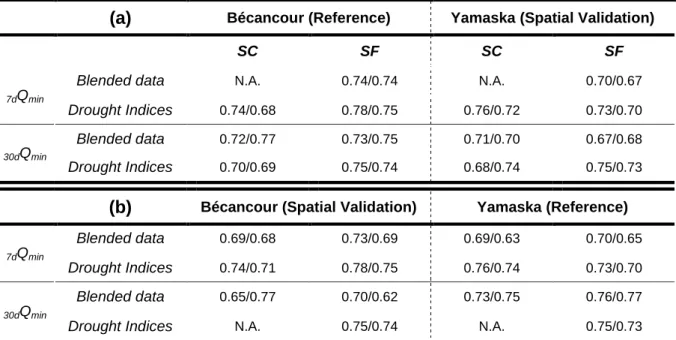
3.2.2 CDI governing low flows
536Table 5 introduces the results obtained after application of the methodological framework 537
introduced in Figure 1. The Bécancour watershed was first considered as the reference and 538
the CDIs are exported onto the Yamaska watershed for a spatial validation and vice versa. 539
Table 5: Pearson median correlations r (Past temporal horizon/Future temporal horizon) after application
540
of the methodological framework using (a) Bécancour as the reference watershed and then (b) Yamaska
541
as the reference watershed
542
(a)
Bécancour (Reference) Yamaska (Spatial Validation)SC SF SC SF
7dQmin
Blended data N.A. 0.74/0.74 N.A. 0.70/0.67
Drought Indices 0.74/0.68 0.78/0.75 0.76/0.72 0.73/0.70
30dQmin
Blended data 0.72/0.77 0.73/0.75 0.71/0.70 0.67/0.68
Drought Indices 0.70/0.69 0.75/0.74 0.68/0.74 0.75/0.73
(b)
Bécancour (Spatial Validation) Yamaska (Reference) 7dQminBlended data 0.69/0.68 0.73/0.69 0.69/0.63 0.70/0.65
Drought Indices 0.74/0.71 0.78/0.75 0.76/0.74 0.73/0.70
30dQmin
Blended data 0.65/0.77 0.70/0.62 0.73/0.75 0.76/0.77
Drought Indices N.A. 0.75/0.74 N.A. 0.75/0.73
N.A. stands for CDI-HDI couples that passed the Wilcoxon rank-sum test and thus did not respect the
543
hypothesis according to which median correlations should remain the same between past and future
544
horizons
545
Overall, when Bécancour was the reference watershed, the explained variability (r²) for the 546
Yamaska watershed was greater than 45% (0.67²) for the 7dQmin and the 30dQmin for both 547
temporal horizons. When Yamaska was used as the reference watershed, the explained 548
variability for Bécancour past horizon varied between 42 (0.65²) and 61% (0.78²). Meanwhile 549
for the future horizon, it varied between 38 (0.62²) and 59% (0.76²). The differences between 550
parts (a) and (b) of Table 5, where the watersheds were in turn used for calibration or spatial 551
validation, are not statistically significant, except for the SF season 30dQmin blended data CDI 552
for both temporal horizon and the future only respectively for the Yamaska and Bécancour 553
watersheds, according the Wilcoxon rank-sum test at 5% significance level. This means that 554
it cannot be asserted that performances are significantly different for the same watershed, 555
whether it is used as the reference or export watershed. This result can hardly be seen as a 556
proof that the statistical relationship captured on a watershed is applicable to another, but it 557
provides a good insight as for the potential of this method for regionalization studies. 558
Moreover, the differences in performances might be larger if the considered watersheds were 559
in different geological areas or further away from each other physiographically speaking. 560
These two points would mandate for the application of the methodological framework on 561
other watersheds to assess the robustness with regards to physiographical differences. 562
However, in terms of hydrologic model performance rating (Moriasi et al., 2007), the median 563
Pearson correlation coefficients were considered “acceptable” since they were all greater 564
than 0.5 (Santhi et al., 2001; Van Liew et al., 2003), even for the great majority of 1st deciles. 565
As anticipated, the results are quite similar for the two studied watersheds. Indeed, the study 566
focused on identifying the main governing indices of low flows while building on the 567
assumption that physical links between HDIs and CDIs remained time invariant (between 568
past and future horizons). As such, this approach may be viewed as the temporal equivalent 569
of the global calibration strategy of distributed hydrological models (Ricard et al., 2013). It 570
was notably used in CEHQ (2013b, 2015) to ensure the spatial consistency of the calibration 571
parameter sets in large-scale hydrological modeling applications. Meanwhile the choice to 572
work with best median correlations for each type of input data in this paper ensured that the 573
identified CDIs in subsection 3.2.2 were valid for each of the 42 climate scenarios. 574
Following the methodological framework introduced in Figure 1, the CDIs from the blended 575
data and drought indices groups that are better correlated with the HDIs (Figure 6) are 576
identified hereafter. For both study watersheds, the severity of 7-day low flows of the SC 577
season was best correlated with the EDI computed from rainfall and snowmelt minus PET 578
amounts over 10 months. SC season 30-day low flows were best correlated with the same 579
index, but over the course of 10 and 12 months for the Yamaska and Bécancour watershed, 580
respectively. The latter result is rather logical, given that 30-day-low flows can mobilize more 581
water reserves than 7-day-low flows. It is noteworthy that the accumulation of rainfall and 582
melt over three months and rainfall plus melt minus PET over two months are also correlated 583
with the 30-day low flows of the Bécancour and Yamaska watersheds, respectfully. This 584
would highlight the importance of working at different time scales as CDIs computed from 585
blended data seem best correlated at lower frequencies than drought indices CDIs. Indeed, 586
the same observation can be made for the CDIs computed for the SF season. 587
SF season 7- and 30-day-low flows were correlated with cumulative climatic demand over 588
four to six months, indicating that lower rainfall amounts or higher PET amounts would 589
translate into lower low flows. The specific case of the inclusion of melt in the CDI computed 590
for the Yamaska watershed for the SF season 30dQmin may be startling. But in fact, this result 591
is linked with the depletion of groundwater storage. Accumulation of rainfall over a month is 592
the primary CDI driver (for precipitation data CDI) of 30dQmin with a median correlation of 0.72 593
(shown in supporting material 4) and 1st and 9th deciles of 0.35 and 0.83. Accumulation of 594
rainfall and snowmelt over a month is the primary CDI driver (for blended data) of 30dQmin with 595
a median correlation of 0.76 ((b) Table 5) and 1st and 9th deciles of 0.52 and 0.84. The 596
difference in median correlations is not significant, but the difference in the 1st deciles is. This 597
could be interpreted as follows: When melt occurs shortly (less than a month) before the date 598
of occurrence of the 30dQmin, the stored amount of snowmelt helps relieve the severity of low 599
flows, but this happened rarely over the 42 scenarios (1st decile difference). Another 600
explanation could be that man-made reservoirs are mainly filled thanks to snowmelt. Last but 601
not least, this result could not be random for two reasons: (i) this phenomenological 602
observation, however less important, manifested also for the Bécancour watershed ((b) 603
Table 5), the correlations for 30dQmin blended data are 0.70 and 0.62 for the past and future 604
horizons); and (ii) the 95% CI for the true value of the median correlation coefficient for the 605
Yamaska watershed is [0.72 – 0.81] (supplemental material 4). 606
Otherwise, SF season 7- and 30-day-low flows were best correlated with EDI computed from 607
climatic demand over 6 months for both watersheds. 608
3.3 HDI trends and their possible drivers
– trend detection and partial
609
correlation analysis
610
Trend analyses of the HDI and associated CDI series were undertaken to check for long term 611
changes, thanks to the modified MK test (Hamed and RamachandraRao, 1998). Field 612
significance was assessed, applying a bootstrap resampling method based on Monte Carlo 613
simulations. Both local significance and field significance were set at 1%. An overview of the 614
results for the ten continuous scenarios is given in Table 6. Indeed, data from the 32 non-615
continuous scenarios came in two 29-year temporal horizons, which in most cases prevented 616
the detection of positive or negative trends altogether 617
Table 6 : Trends detected in the HDI and CDI series for the (a) Bécancour and (b) Yamaska watersheds for
618
the 10 scenarios by Ouranos over 1971-2070. CDI1 stands for the CDI computed from blended data, while
619
CDI2 stands for CDI computed from drought indices. Bold figures indicate significant trends.
620
(a) Bécancour
Snow Cover Season Snow Free Season
7dQmin
HDI – CDI1 – CDI2 HDI – CDI1 – CDI2 30dQmin HDI – CDI1 – CDI2 7dQmin HDI – CDI1 – CDI2 30dQmin Positive trends 10 – N.A. – 10 10 – 10 – 10
Negative trends 8 – 8 – N.A. 8 – 8 – 8
Significant trends (positive & negative)
10 – N.A. – 10 10 – 10 – 10 8 – 8 – N.A. 8 – 8 – 8
(b) Yamaska
Snow Cover Season Snow Free Season
7dQmin
HDI – CDI1 – CDI2 30d
Qmin
HDI – CDI1 – CDI2 7d
Qmin
HDI – CDI1 – CDI2 30d
Qmin
HDI – CDI1 – CDI2
Positive trends 9 – N.A. – 10 10 – 10 – 10 0 – 1 – 0
Negative trends 7 – 8 – 10 7 – 2 – 9 Significant trends (positive & negative) 9 – N.A. – 10 10 – 10 – 10 7 – 8 – 10 7 – 3 – 9 621
Table 7 : Pearson median partial correlation coefficients r (Past horizon/Future Horizon/1971-2070) for the
622
Bécancour and Yamaska watersheds for the CDIs obtained after application of the methodological
623
framework for the 10 scenarios by Ouranos. CDI1 stands for the CDI computed from blended data, while
624
CDI2 stands for CDI computed from drought indices.
625
(a) Bécancour Watershed
SC season SF season
CDI1 CDI2 CDI1 CDI2
7dQmin N.A. 0.74/0.65/0.68 0.71/0.61/0.68 N.A.
30dQmin 0.77/0.75/0.73 0.69/0.62/0.64 0.70/0.73/0.70 0.66/0.66/0.66
a (b) Yasmaka Watershed
CDI1 CDI2 CDI1 CDI2
7dQmin N.A. 0.78/0.71/0.74 0.73/0.71/0.66 0.62/0.63/0.58
30dQmin 0.74/0.78/0.73 0.73/0.75/0.72 0.73/0.72/0.63 0.71/0.63/0.61
All partial correlation coefficients are significant at 0.001.
626
Both Bécancour and Yamaska SC 7dQmin as well as 30dQmin have increasing linear significant 627
trends (Table 6) as indicated by CEHQ (2015) for most of southern Québec with a high 628
confidence level. These trends are probably linked to an increase in freeze/thaw events or 629
warm events during the SC season (included in supporting material 2) and as a direct 630
consequence, modified snowmelt dynamics. The associated CDIs, whether computed from 631
blended data or drought indices, also displayed these increasing trends (Table 6). They were 632
in almost perfect agreement with the HDI trends. Meanwhile, the partial correlations 633
removing the temporal trends were not only significant (Table 7 and 95% CI available in 634
supporting materials 3 and 4), but quite high as well. Indeed, the CDIs explained more than 635
48 (0.69²) and 38% (0.62²) of the HDI variability for the Bécancour watershed over the past 636
and future temporal horizons, respectively. Values were even larger for the Yamaska 637
watershed with at least 53 (0.73²) and 50% (0.71²) of the HDI variability explained for the 638
past and future horizons, respectively. Overall, compared to median Pearson correlations for 639
the same CDIs and the 10 continuous scenarios, median partial correlations (supporting 640
material 5) were only 3.2% smaller on average with a maximum difference of 6.8% for the 641
SC season Bécancour CDIs. These partial correlations values are large, the lower bound of 642
the 95% CI (supporting materials 3 and 4) is still considered “acceptable” (larger than 0.5 643
(Santhi et al., 2001; Van Liew et al., 2003)) in terms of hydrologic performance rating
644
(Moriasi et al., 2007), and the associated trends in the CDIs were in almost perfect
645
agreement with the HDI trends (Table 6). Given these results, it is then possible to attribute 646
the observed trends in SC low flows to trends in the CDIs identified in subsection 3.2.2 for 80 647
to 100% of the climate scenarios. 648
The same reasoning can be made about the SF season low flows. 70 and 80% of the 649
decreasing trends in HDIs were significant and concurred with results reported in CEHQ 650
(2015) for southern Québec. The associated CDIs had matching trends (except for the CDI 651
computed using blended data for the Yamaska 30dQmin in Table 6), while the partial 652
correlations between the HDIs and CDIs were high (above 0.62 for the past temporal horizon 653
and above 0.61 for the future temporal horizon) and the lower bounds of their 95% CI 654
remained “acceptable”. Given these results, it is then possible to attribute the observed 655
trends in SF low flows to trends in the CDIs identified in subsection 3.2.2 for 70 to 100% of 656
the climate scenarios. 657
4. Discussion
658The following section deals with the relevance of the main assumptions made throughout the 659
paper, more specifically it: (i) shows how sources of climate uncertainty were considered 660
while selecting the climate simulations and emissions scenarios; (ii) examines the validity of 661
the assumptions regarding the stationarity of climate conditions, land use, and land cover; 662
(iii) details how HDIs and (iv) CDIs actually captured what is observed; (v) discusses the 663
robustness of the results; and (vi) argues the proposed methodology has potential to be 664
applicable to watersheds with regulated flows. 665