A New Concept to Calibrate and Evaluate a Hydrological Model
Based on Functional Data Analysis
Samah Larabi,
1André St-Hilaire
1,2and Fateh Chebana
11Institut National de la Recherche Scientifique, Centre Eau Terre Environnement, Québec City, Québec; 2Canadian Rivers Institute, University of
New Brunswick, Fredericton, New Brunswick.
Abstract
Performance measures are widely used in hydrological modeling to provide objective evaluation of the match between simulated and observed system output (i.e. discharge). Each performance measure emphasises a particular aspect of a hydrograph, and the use of a particular performance measure on a specific metric typically means discounting one aspect at the expense of another (e.g. high flows vs low flows). This is mainly because most performance measures reflect the adequacy of simulations using one calculated value based on residuals between daily or hourly series of simulated and observed streamflows. However, it would be more practical to conserve the temporal flow variability of the entire annual hydrograph than to focus merely on flood peaks, for instance. Functional data analysis is a mathematical tool that allows the comparison of such data. In this paper, a methodology for model calibration and evaluation that considers an annual hydrograph as a single observation instead of 365 daily observations, based on functional data analysis, is proposed. The model is evaluated on its ability to reproduce the same shape and variability as the observed hydrographs. The functional statistics, defined for each time step, are used to construct the objective function for model calibration as well as for further model evaluation. A case study is presented to evaluate the hydrological CEQUEAU model on the Lac St-Jean drainage basin. The concept that we describe is general and can be used with any calibration scheme or model evaluation.
1 Introduction
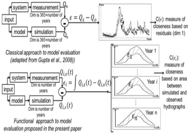
Hydrological model calibration is a complex task. The success of the activity depends on different factors including both the qual-ity and quantqual-ity of available data, the performance measure(s) used to evaluate model adequacy, and the calibration procedure. Performance measures, widely used in hydrological modeling, aim to provide an objective evaluation of the closeness between simulated and observed hydrological data (Pechlivanidis et al. 2010). Each performance measure emphasizes a particular aspect of the hydrograph, or a dynamic behaviour (e.g. low or high flow). Therefore, any performance measure, no matter how carefully chosen or defined, is inadequate to represent the variability of the entire hydrograph (Vrugt et al. 2003; Krause et al. 2005). Gupta et al. (1998) highlight the importance of using different perfor-mance measures simultaneously in order to capture different hydrograph features. However, the majority of the performance measures used (e.g. Nash–Sutcliffe efficiency, NSE; root mean square error, RMSE) compare the simulated and observed stream-flow point by point (daily or hourly stream-flows) and are associated with a loss of information, as illustrated in Figure 1. Recently model
diagnostic evaluation has been used instead of model calibration
(e.g. Gupta et al. 2008; Yilmaz et al. 2008). This approach aims
to examine the extent to which a model can be reconciled with observations, and identifies the model component that needs improvement (Gupta et al. 2008). The approach is based on using
hydrological signatures which are indices describing the different
characteristics of the flow regime in a watershed.
Figure 1 Model evaluation concept with classical performance measure vs the functional approach.
The common limitation of the traditional performance measures such as NSE or RMSE and the hydrological signatures is that information about the temporal flow variability is lost. Streamflow is naturally continuous in time. Therefore, it is more realistic to compare the entire simulated and observed hydro-graphs as temporal functions instead of discrete (daily or hourly) observations. The functional framework introduced by Ramsay and Silverman (2002; 2005) allows the study and performance of statistical analysis on such data (i.e. hydrographs as tempo-ral functions). Functional data analysis (FDA) is widely used in different fields (Ramsay and Silverman 2002). In hydrology, this framework was used for flood frequency analysis and outlier de-tection by Chebana et al. (2012), for hydrograph classification by Ternynck et al. (2016); and for streamflow forecasting by Masselot et al. (2016). FDA allows the modeller to conduct one analysis of the entire data, transformed into a function, instead of several univariate or multivariate analyses (Chebana et al. 2012).
The objective of this study is to define a performance measure based on FDA that preserves the temporal flow variabil-ity. The proposed conceptual framework for model evaluation consists of comparing the observed and simulated hydrographs as single entities, as illustrated in Figure 1 above. The time series in this context are temporal curves of dimension n (number of years of observations), unlike in the classical approach where the time series are a vector of dimension 365 × n. The model
evalu-ation is based on functional statistics that are provided by time step and would represent an extension of traditional hydrological signatures in the context of functional data.
The novelty of this paper is using the FDA framework as a tool for hydrological model calibration and evaluation that allows an analysis of the simulated and observed hydrographs in one single step. In contrast, the classical approach requires multiple analyses to study low and high flows and timing to peak flows.
FDA is introduced in section 2 together with a description of the conceptual framework used to calibrate a model using this tool. Section 3 provides a case study of applying this concept to calibrate a hydrological model. Section 4 provides results and dis-cussion on using the FDA for model evaluation and possible ways forward, followed by conclusions in section 5.
2 Methods
2.1 Converting Discrete Data to Functional Data
Converting raw data (discharge observations in our case) to func-tional data is the preliminary step in FDA. It consists of smoothing the original discrete data by a basis expansion. For a given annual series of daily discharge, Yi = {Y(i,1), …, Y (i,365)} is converted to a continuous temporal function denoted xi(t) and defined for eachtime step t in [1, T = 365]:
xi
( )
t = k=1ck∅k K∑
(1)where:
Øk = the basis functions,
ck = the coefficients, and
K = the number of basis functions.
There are several basis functions (e.g. constant, polynom-ial, spline, Fourier series, wavelets) adapted for each case study and type of data. In this study, the data (daily discharges) are periodic; hence it is adequate to use a Fourier series (similar to Chebana et al. 2012). The basis coefficients ck are to be estimated by a least square error or a penalized least square error in order to adequately fit the data (Ramsay and Silverman 2002). In fact, the greater K is, the lower the bias is (constructed curves exactly match the data). In contrast, the lower K is, the more the fitted curves are smooth at the expense of catching sharper features of the data (Levitin et al. 2007). In this study, FDA is used for calibra-tion purposes where the aim is to capture the maximum of infor-mation about the flow dynamic while leaving out some spurious noise. Therefore, a penalized least square error is privileged be-cause it allows fixing a large number K of basis functions and add-ing a roughness penalty. Details on smoothadd-ing data can be found in Ramsay and Silverman (2002; 2005). Smoothing parameters are chosen so that important features of the original observed series (e.g. peak flows) are not lost through smoothing.
2.2 Exploring and Analyzing Functional Data
Clausen and Biggs (2000) defined three groups of flow variables that characterize a flow regime:1. general flow variables (including mean and median flow, skewness and coefficient of variation); 2. high flow variables (e.g. peak flow, 10% and 20%
ex-ceedance flows read from the flow duration curve); and
3. low flow variables (e.g. 90% exceedance flow read from the flow duration curve).
These flow variables are commonly used for hydrological model diagnostics (e.g. Yilmaz et al. 2008; Euser et al. 2013; Shaffi and Tolson 2015). In this study, we can define general flow vari-ables based on the functional statistics that are defined by time step. For a sample of curves X={xi (t), t ε τ=[1, ...T], (here T=365), i =
1, …, n:number of years}, the mean function is:
X = 1
n i=1xi (t
),
t∈ τ
n∑
(2)The median is defined, in the functional context, based on a depth function notion. The depth function was introduced by Tukey (1975) for ordering multivariate data. In functional con-texts, it is used as a measure of location and dispersion. The medi-an curve is the deepest function in the sample medi-and maximizes the depth function Dn(X):
Xmedian= argmax
X∈{X1, …, Xn}Dn
( )
X(3)
varX [X(t)] = 1 n−1
(
)
i=1(
xi (t)− X)
n
∑
2, t ∈ τ (4)Other statistics can be explored, such as the modal curve, the trimmed mean and the covariance function (given by Chebana et al. 2012). Based on the standard deviation curve (the square root of the variance curve) and the mean curve, one can define a coefficient of variation for each time step, which is the standard deviation divided by the mean flow. The fact that these statistics are given by functions allows for the representation of the temporal variability of these statistics and thus allows for the description of the entire streamflow variability (high and low flows) in one single step and so there is no need for high or low flow variables as defined by Clausen and Biggs (2000).
With the functional Student test, a comparison between two samples X1 and X2 of curves can be made for each time step t. The functional Student statistic is defined for each time step t as:
t statistic = X1−X2 1 T var X
{
[
1( )
t]
+var X[
2( )
t]
}
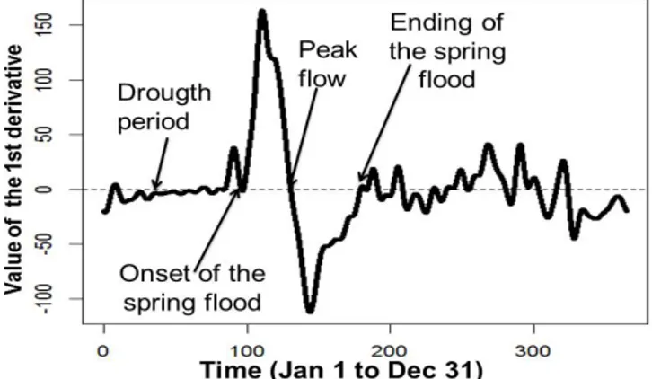
(5)The FDA also allows for analysis of the derivatives of the curves. The first derivative indicates the timing of the hydrological events such as the onset of the spring flood, the peak flow or drought, as illustrated in Figure 2. In fact, the intersection points of the first derivative curve with the x–axis (i.e. derivative = 0) indicate the days when a minimum or maximum occurred. Posi-tive first derivaPosi-tive values indicate an increase in the streamflow, which is the rising limb of the hydrograph. In contrast, negative values indicate a decrease in the streamflow, which is the reces-sion curve.
Figure 2 Extracting timing of hydrological events from the first derivative of annual hydrograph.
2.3 Defining an Objective Function
In this study, each annual daily discharge series {y(i,1), …, y(i,365)} is converted into one single observation, which is the smoothed hydrograph Qi(t), t ε [1, T = 365]. The framework we propose includes an evaluation of the ability of the model to reproduce annual hydrographs that are as close as possible to the observed one, as illustrated in Figure 1. One means of comparison between a simulated and an observed hydrograph is to compare the
sur-faces under each curve (i.e. the volume). The objective function can then be expressed as:
ofi=1− Q
∫
i ,sim (t)
dt
∫
Qi , obs (t)dt (6)where Qi,sim(t) and Qi,obs(t) are the simulated and observed
smoothed hydrographs respectively as defined in Equation 1 using a Fourier series as basis functions.
For model evaluation over a selected period (N years), this objective function is computed for each year i. The global per-formance of the model can be measured as the sum of these an-nual objective functions over the selected period. For calibration purposes and to ensure that the model provides accurate flows for each time step (during both low flow and high flow phases), the objective function can be weighted by the average of the functional Student statistic. If a set of model parameters fails to simulate a portion of the hydrograph, this weighting criterion is automatically high. Thus, the objective function is amplified and the set containing the parameter in question is rejected. The ob-jective function is:
OF = S× i=1ofi
N
∑
(7)where :
ofi = as defined in Equation 6,
S = the mean of the Student test statistic given by
Equation 5, and
N = the number of years of observations.
An alternative is to examine the result vector
OF = {of1, …, ofi, …, ofn}; that is, to simultaneously optimize ofi with a multi-objective algorithm.
3 Case study
3.1 Model and Data Description
CEQUEAU is a deterministic semi-distributed hydrological model that simulates and predicts streamflow at any point of a grid that covers a watershed (Charbonneau et al. 1977; St-Hilaire et al. 2000; Morin and Paquet 2007). The model takes into account the physical characteristics of the watershed by decomposing it into equal squares called whole squares. For each whole square the altitude and the percentages of forest cover, lakes and wetlands are defined and the vertical routing is simulated by a produc-tion funcproduc-tion. The available water volume on each whole square is then routed downstream by a transfer function. A detailed description of the model is given by Morin and Paquet (2007). CEQUAU has 28 parameters that are adjusted in order to simulate flows that match as closely as possible the observed flows. In this study, only 10 parameters (describing snow accumulation, snowmelt, infiltration, interflow, surface runoff and evaporation) are adjusted. These parameters are the most sensitive parameters. The other parameters are fixed based on previous calibration.
sample is generated, Y (2000 sets of parameters), from the space defined by the bounds of X*. From the set Y, the subset of the deepest points, Y*, within X* are selected. Sets of parameters hav-ing depth superior to the median of the depths are considered to be deep. For the next iteration the set Y* becomes X and the process is repeated until the performance of Y* does not improve any more. The space defined by the final Y* is considered to be the optimal space.
The second step of the procedure aims to explore in depth the optimal space inferred from the Monte Carlo simulation. At this step, a basic version of the Tabu search (Glover 1990; Glover and Laguna 1997) is used. The Tabu algorithm starts with an initial set of parameters, evaluates its neighbouring sets of candidates and replaces it with the best candidate set according to the objective function defined in Equation 7 until a stop criterion is satisfied. The algorithm uses a first-in–first-out list, called a Tabu list, that aims to prevent the search from re-evaluating sets of pa-rameters that were already examined. Thus it prevents the algo-rithm from stopping at the first optimum found or being trapped in repetitive cycles.
4 Results and Discussion
To evaluate the calibrated model, the model is evaluated based on the statistics given in subsection 2.2. Figure 4 shows the simulated and observed interannual mean values with the asso-ciated results of the Student test in the calibration and validation periods. The model provides a good simulation of the rising limb of the hydrographs as well as the recession curves. However, it underestimates the spring flood volume in both the calibration and the validation periods. Overall, the Student test shows the capability of the calibrated model to produce flows similar to the observed flows for any period of the year. The Student statistic is lower than the p-value represented by the dashed line for almost every time step.
Figure 4 The observed and simulated hydrographs with the associated Student test in calibration and validation periods.
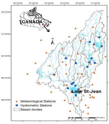
The model is calibrated on the Lac St-Jean drainage basin located in the province of Québec (Figure 3). This watershed covers an area of 73 800 km2 with 90% forest cover and altitude ranging from 88 m to 792 m. The flow regime is typical of nordic basins where the main source of streamflow is the snowmelt dur-ing sprdur-ing. The main source of streamflow durdur-ing winter is from groundwater discharge. The maximum flow reaches 6733 m3/s. The mean annual precipitation varies from 837 mm to 1046 mm in the watershed. Only the flowgauge at the outlet of the water-shed was used for calibration in the present study. Discharge data from 2001 to 2013 were used for model calibration and evalua-tion. The first year (2001) was used as a warm-up period, the next eight years (2002-2009) were used for calibration, and the remain-ing four years were used for model validation.
Figure 3 The Lac St-Jean drainage basin.
3.2 Model Identification
To adjust the model parameters a two-step approach is used. The first step aims at defining an optimal parameters space using a Monte Carlo uniform random search with a depth function, adapted from Bardossy and Singh (2008). The methodology aims to direct the sampling of parameters into the zone where the sets of parameters leading to good model performance are located, through a depth function. Depth functions are statistical tools that allow the user to quantify the centrality of a point within a multivariate cloud of data (Zuo and Serfling 2000). The principle of the methodology is as follows. An initial sample X (1000 sets of parameters) is generated from the initial parameter space and evaluated using the objective function defined in Equation 7. The 100 (10%) best sets of parameters, X*, are selected. A second
Figure 5 shows the coefficient of variation for each time step for both calibration and validation periods. It shows that the model fails to simulate the same variability for winter flows (flows observed from day 1 to day 90) as well as for autumn (fall) flows (day 310 to day 355). For the rest of the year the model well matches the flow variability.
Figure 5 Coefficient of variation of the simulated and observed flows for the calibration and validation periods.
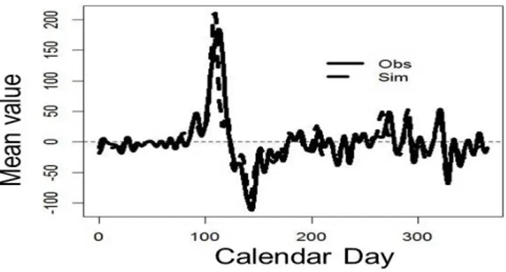
Figure 6 presents the first derivative of the simulated and observed mean hydrographs. The model well matches the timing to the onset of the flood curve and the timing to the peak flow. The simulated first derivative curve show good synchronicty to the observed curve, which reveals a good synchronicity between observed and simulated flows.
Figure 6 The average curves of the first derivatives of the simulated and observed hydrographs during calibration period.
In order to confirm the accuracy of the conclusions drawn from the functional analysis, we examine the time series. Figure 7 and Figure 8 present the simulated and observed flow time series during the calibration and validation periods. The simulated flows show a good synchronicity with the observed flows, with NSE values of 0.89 during calibration and 0.93 during validation. The relative bias is 2% during the calibration period and 4% during the validation period. During the calibration period the model underestimates the peak flows of large spring floods, which ex-plains the underestimation of flood volume (Figure 4). During the validation period, the calibrated model does not catch the spring flood volume of the year 2011 and underestimates the peak flow of year 2013. The other years are well simulated. Because the flow series are short for the validation period (only 4 y), the interannual
flow is influenced by the large flood events of the years 2011 and 2013. This explains the high bias seen in Figure 4 between the simulated and observed interannual means during spring.
Figure 7 Time series of observed and simulated flows during calibration period.
Figure 8 Time series of simulated and observed flows during validation period.
In this paper, we illustrated the advantages using FDA for model evaluation. This tool provides a full and complete descrip-tion of the whole hydrograph in one single step, unlike conven-tional statistics. The use of funcconven-tional statistics allows recognition of the times during which the model fails to adequately simulate the observed system behaviour; thus it allows identification of the model components that need further adjustment. In the case study the calibrated model preserves the hydrograph mean but fails to accurately simulate the low flow variability during winter. Overall the calibrated model provides accurate simulation of low and high flows, according to the Student test, and as shown by visual comparison of the simulated and observed time flow series. In this study, only parameters controlling the snow accumulation, snowmelt, and coefficient of drainage are adjusted while the drainage thresholds are fixed. Further calibration of these drain-age thresholds might improve the flood volume simulation.
The conceptual framework presented in this paper can be extended to include uncertainty analysis by relating the objective function to the parameter distributions. It can also be extended to a multi-objective framework as explained in subsection 2.3. By doing so, the model is calibrated in such a way that it is able to capture the different hydrograph shapes resulting from climate variability.
5 Conclusions
This paper introduces alternatives to conventional performance measures and flow variables that are associated with a loss of information, in particular the temporal flow variability. This paper presents ways to use the FDA framework in the context of model evaluation. The entire hydrograph is considered as a single ob-servation and the model is evaluated on its ability to reproduce the shape and variability of the observed hydrograph. The case study presented illustrates the potential application of using this tool for model calibration to estimate both low and high flows. The proposed conceptual framework can be adapted to calibrate the model on selected parts of the hydrograph (i.e. for an event-based calibration), depending on the intended use of the model. Further work is needed to integrate this tool within a complete uncertainty analysis.
Acknowledgment
The authors acknowledge the financial contribution of Rio Tinto, NSERC and MITACS.
References
Bardossy, A. and S. Singh. 2008. “Robust Estimation of Hydrologic-al Model Parameters.” HydrologicHydrologic-al Earth System Sciences 12:1273–83.
Charbonneau, R., J. Fortin and G. Morin. 1977. “The CEQUEAU Model: Description And Examples of its Use in Problems Related to Water Resource Management.” Hydrological
Sci-ences Bulletin 22 (1): 193–202.
Chebana, F., S. Dabo-Niang and T. B. M. J. Ouarda. 2012. ”Explora-tory Functional Flood Frequency Analysis and Outlier De-tection.” Water Resources Research 48.
https://doi.org/10.1029/2011WR011040
Clausen, B. and B. J. F. Biggs. 2000. “Flow Variables for Ecological Studies in Temperate Streams: Groupings Based on Covari-ance.” Journal of Hydrology 237:184–97.
https://doi.org/10.1016/S0022-1694(00)00306-1
Euser, T., H. C. Winsemius, M. Hrachowitz, F. Fenicia, S. Uhlenbrook and H. H. G. Savenije. 2013. “A Framework to Assess the Realism of Model Structures Using Hydrological Signatures.”
Hydrological Earth System Sciences 17:1893–912.
https://doi.org/10.5194/hess-17-1893-2013
Glover, F. 1990. “Tabu Search: A Tutorial.” Interfaces 20:74–94. Glover, F. and M. Laguna. 1997. Tabu Search. Boston, MA: Kluwer
Academic.
Gupta, H. V., S. Sorooshian and P. Yapo. 1998. ”Toward Improved Calibration of Hydrological Models: Multiple and Noncom-mensurable Measures of Information.” Water Resources
Research 34 (4): 751–63.
https://doi.org/10.1029/97WR03495
Gupta, H. V., T. Wagener and Y. Liu. 2008. “Reconciling Theory with Observations: Elements of a Diagnostic Approach to Model Evaluation.” Hydrological Processes 22:3802–13.
https://doi.org/10.1002/hyp.6989
Krause, P., D. P. Boyle and F. Bäse. 2005. “Comparison of Different Efficiency Criteria for Hydrological Model Assessment.”
Ad-vances in Geosciences 5:89–97.
https://www.adv-geosci.net/5/89/2005/adgeo-5-89-2005. pdf
Levitin, D., R. Nuzzo, B. Vines and J. O. Ramsay. 2007. “Introduction to Functional Data Analysis.” Canadian Psychology 48 (3): 135–55.
https://doi.org/10.1037/cp2007014
Masselot, P., S. Dabo-Niang, F. Chebana and T. B. M. J. Ouarda. 2016. “Streamflow Forecasting Using Functional Regres-sion.” Journal of Hydrology 538:754–66.
https://doi.org/10.1016/j.jhydrol.2016.04.048
Morin, G. and P. Paquet. 2007. Modèle hydrologique CEQUEAU. Québec: Institut national de la recherche scientifique. Rap-port de recherché, INRS-ETE, no R000926.
http://espace.inrs.ca/1098/1/R000926.pdf
Pechlivanidis, I. G., B. Jackson and H. McMillan. 2010. “The Use of Entropy as a Model Diagnostic in Rainfall–Runoff Model-ing.” Presented at 5th International Congress on Environ-mental Modeling and Software—Ottawa, Ontario, Canada, July 2010: Modeling for Environment’s Sake. Manno: iEMSs (International Environmental Modeling and Software Soci-ety).
https://scholarsarchive.byu.edu/iemssconference/2010/ all/325
Ramsay, J. O. and B. W. Silverman. 2002. Applied Functional Data
Analysis: Methods and Case Studies. New York: Springer.
Ramsay, J. O. and B. W. Silverman. 2005. Functional Data Analysis, 2nd ed. New York: Springer.
Shafii, M. and B. A. Tolson. 2015. “Optimizing Hydrological Con-sistency by Incorporating Hydrological Signatures into Model Calibration Objectives.” Water Resources Research 51. https://doi.org/10.1002/2014WR016520
St-Hilaire, A., G. Morin, N. El-Jabi and D. Caissie. 2000. “Water Tem-perature Modeling in a Small Forested Stream: Implication of Forest Canopy and Soil Temperature.” Canadian Journal
of Civil Engineering 27:1095–1108.
https://doi.org/10.1139/l00-021
Ternynck, C., M. A. Ben Alaya, F. Chebana, S. Dabo-Niang and T. B. M. J Ouarda. 2016. ”Streamflow Hydrograph Classification Using Functional Data Analysis.” Journal of
Hydrometeoro-lolgy 17 (1): 327–44.
https://doi.org/10.1175/JHM-D-14-0200.1
Tukey, J. W. 1975. “Mathematics and the Picturing of Data.” In
Proceedings of the International Congress of Mathematicians, Vancouver, 1974, 523–31. Montreal: Canadian Mathematical
Vrugt, J. A., H. V. Gupta, L. A. Bastidas, W. Bouten and S. Sorooshian. 2003. ”Effective and Efficient Algorithm for Multiobjective Optimization of Hydrologic Models.” Water
Resources Research 39 (8).
https://doi.org/10.1029/2002WR001746
Yilmaz, K. K., H. V. Gupta and T. Wagener. 2008. “A Process-Based Diagnostic Approach to Model Evaluation: Application to NWS Distributed Hydrologic Model.” Water Resources
Re-search 44 (9).
https://doi.org/10.1029/2007WR006716
Zuo ,Y. and R. Serfling. 2000. “General Notions of Statistical Depth Functions.” The Annals of Statistics 28 (2): 461–82.