Systèmes auxiliaires pour les observables : approximation du connecteur dynamique locale pour les spectres d'addition et d'émission d'électrons

(1)

HAL Id: tel-01803435

https://pastel.archives-ouvertes.fr/tel-01803435

Submitted on 30 May 2018

HAL is a multi-disciplinary open access

archive for the deposit and dissemination of sci-entific research documents, whether they are pub-lished or not. The documents may come from teaching and research institutions in France or abroad, or from public or private research centers.

L’archive ouverte pluridisciplinaire HAL, est destinée au dépôt et à la diffusion de documents scientifiques de niveau recherche, publiés ou non, émanant des établissements d’enseignement et de recherche français ou étrangers, des laboratoires publics ou privés.

Systèmes auxiliaires pour les observables :

approximation du connecteur dynamique locale pour les

spectres d’addition et d’émission d’électrons

Marco Vanzini

To cite this version:

Marco Vanzini. Systèmes auxiliaires pour les observables : approximation du connecteur dynamique locale pour les spectres d’addition et d’émission d’électrons. Matière Condensée [cond-mat]. Université Paris Saclay (COmUE), 2018. Français. �NNT : 2018SACLX012�. �tel-01803435�

(2)

NNT: 2018SACLX012

T

HÈSE DE

D

OCTORAT

de

L’UNIVERSITÉ

PARIS–S

ACL AY préparée à

L’

É

COLE

P

OLY TECHNIQUE

École doctorale n°572

Ondes et Matières (EDOM) Spécialité: PHYSIQUE

par

Marco V

ANZINI

Auxiliary systems for observables:

dynamical local connector approximation

for electron addition and removal spectra

Thèse présentée et soutenue à Palaiseau le 30 janvier 2018 devant le jury composé de : Prof. Eric CANCÈS Président du jury

Prof. Eberhard K. U. GROSS Rapporteur

Prof. Nicola MARZARI Rapporteur

Prof. Roi BAER Examinateur

Prof. Silvana BOTTI Examinatrice

Prof. Simo HUOTARI Examinateur

Dr. Lucia REINING Co–encadrante

(3)

(4)

(5)

(6)

Table of main symbols and conventions

r real space vector

n(r ), ¯n local and average densities

nmin, nmax minimum and maximum densities

ωP=

p

4πn plasma frequency in the homogeneous electron gas

rs Wigner–Seitz radius

k reciprocal space vector

εk one–particle excitation energy

G reciprocal lattice vector

{|n,k〉} Bloch basis, with n band index

ϕn,k(r ) = ei k·run,k(r ) Bloch wavefunction

kF Fermi wave vector

vC(r ) Coulomb potential

vext(r ) external potential

vH(r ) Hartree potential

EH Hartree energy

Ex Fock energy

γ(r ,r0₎ _{one–particle reduced density matrix}

n2(r , r0) pair density

nxc(r , r0) exchange–correlation hole

vKS(r ) Kohn–Sham potential

v_KSxc(r ) exchange–correlation part of the Kohn–Sham potential εKS

l ,ϕ KS

l (r ) Kohn–Sham eigenvalue and eigenfunction

φ work function

W bandwidth

α parameter of the PBE0 functional

λ screening length of the HSE06 functional

|Ψ₀N〉 ground state of the N –electron system

E0 ground state total energy

|ΨNs 〉 excited state s of the N –electron system

(11)

εs excitation energy

εc= −EA (minus) electron affinity

εv= −IP (minus) ionization potential

µ chemical potential / Fermi energy

Eg fundamental gap

ω frequency/energy

ˆ

cl, ˆc†_l annihilation and creation operators

ˆ

ψ(r ), ˆψ†_{(r )} _{field operators}

G(r t , r0_t0_{), G(r , r}0_,_ω) _{one–particle Green’s function}

fs(r ) Lehmann amplitude

A(r , r ,ω) spectral function

Σ(r ,r ,ω) exchange–correlation self energy

Z renormalization factor

vSF(r ,ω) spectral potential

v_SFxc(r ,ω) exchange–correlation part of the spectral potential vSR_x (r ,ω) purely frequency–dependent

part of the HSE06 spectral potential vSK(r ,ω) Sham–Kohn quasi particle potential

t , U hopping parameter and interaction strength in the Hubbard model

Gi i(ω) = Gloc(ω) on–site Green’s function

GAIM(ω) impurity Green’s function

∆(ω) impurity hybridization function

G0(ω) impurity reference Green’s function

P .V .Z principal value of the integral

Re, Im real and imaginary parts

sign signum

θ(x) = (

0 if x < 0

1 if x > 0 Heaviside theta function

Fourier transforms: f (y,τ) = Z _dω 2π d3k (2π)3e −i (ωτ−k·y)_{f (k,}_ω) f (k,ω) = Z

d3ydτei (ωτ−k·y)f (y,τ) Continuum limit: 1 V X k → Z _d3_k (2π)3 viii

(12)

IV. Nous suivons le passage le long du mur.

Il y a du monde, chacun est porteur du terme manquant d’une équation destinée à rester sans solution. [...] IX. On ne peut voir le mur que par parties,

la totalité est dans l’esprit. Le texte ne devient complet

que lorsque vous arrivez à la crypte. [...] XI. Certains murs vous incitent à demander: qu’y a-t-il de l’autre côté ?

Ces murs-ci ne décrivent que leur propre limite. Ils vous saisissent, mais ne vous demandent rien.

JOSEPH KOSUTH ‘ni apparence ni illusion’ Murs de l’enceinte de Paris Carrousel du Louvre

(13)

(14)

This thesis is a story, and real stories hardly go straight. This thesis is no exception: I have tried to condensate in the form of a sequential manuscript three years of research, attempts, many errors, new ideas, trials, some successes, some results, a bit of philosophy, discoveries of old ideas, new implementations, models, derivations, ... With these ingredients, I have built this story.

(15)

(16)

Preface

A quoi bon bouger, quand on peut voyager si magnifiquement dans une chaise?

JORIS–KARLHUYSMANS, À rebours

Condensed matter is an amazing field of research. New phenomena periodically pop up out of nature, asking for an interpretation. It is the case of superconductivity, the quantum Hall effect, Mott insulators, excitons, magnons, ...

Remarkably, all of these are emergent phenomena. They cannot easily be explained just by focusing on the properties of the single components involved. On the contrary, they stem from the collective behaviour of particles, which is often more than just the sum of single–particle effects [1].

Typically, an important contribution to these phenomena is provided by electrons.

If in an extended system most of the electrons are usually attached to their nuclei, some of them can move almost freely through the system. These electrons, called valence electrons, wander around, explore and possibly establish coherent connections among themselves. They lose their purely atomic nature, in which their energy is fixed by the atomic quantum numbers n, l, m, and they enter a full many–body realm, where plenty of new energy states are available. Some of these states can be considered as single–particle–like, and the many–electron sys-tem behaves as if it were composed of several quasi–independent electrons with renormalized properties. These are the famous Landau quasiparticles [2], which explain the success of the free electron gas as a model for metals. Some other states cannot definitely be viewed as single– particle–like, and they are the fingerprint of correlations between electrons. These states prove that the many–body system behaves as a whole, and a true many–body approach should be employed for its description.

Such a description exists, it has been developed in the fifties and the sixties, and it relies on the formalism of the Green’s functions [3, 4, 5]. It is a very general theory with several ramifi-cations. It yields, in principle, all the information that one could retrieve from the many–body system (i.e., all the information enclosed in the many–particle wavefunction). It is the theory of everything of condensed matter.

However, one is usually not interested in everything. Something is already enough. In par-ticular, the spectral function alone already offers an excellent characterization of the system. Moreover, the spectral function is a measurable quantity, that can be used to benchmark the theoretical approach.

(17)

PREFACE

theoretical point of view and in an effective way, the spectral function of a many–electron sys-tem, which is measured in photoemission or inverse photoemission spectroscopy.

In particular, throughout the thesis (and explicitly in chapter 1) I refer to angle–integrat-ed photoemission experiments. This is a spectroscopy technique basangle–integrat-ed on the photoelectric effect: schematically, a photon impinges on a sample, it transfers its energy to one of the elec-trons, which is consequently kicked out of the material and finally collected by an analyzer. By measuring the number of detected electrons at different energies, one has a clear map of the energy distribution of the electrons in the material.

Such a map is of fundamental importance, as it establishes a true window on the micro-scopic world of electronic states. Describing this map – if it is available – or predict it – when it is not – is the challenge of theoretical spectroscopy1.

In the Green’s functions formalism I mentioned above, the one–particle Green’s function G(r , r0,ω) exactly describes the physics of charged excitations, in which an electron is removed from (photoemission) or added to (inverse photoemission) the system. While the microscopic description requires the full Green’s function, the comparison with experiments is realized through a much simpler quantity. It is the integrated spectral function A(ω), and it is derived from the Green’s function via the following relation:

A(ω) ∼ 1 V

Z

d3r ImG(r , r ,ω).

This function is the microscopic quantity that makes the link with experiments possible. In the standard approach (described in chapter 2), one first evaluates the full Green’s function G(r , r0,ω), through the introduction of a non–local, complex and frequency–dependent poten-tial, the self energyΣ(r ,r0,ω). Once G(r ,r0,ω) is at hand, all the off–diagonal elements and the real part of the diagonal are discarded. Finally, one integrates ImG(r , r ,ω) over space to obtain A(ω). At the final stage, a lot of information is removed, and one could question the efficiency of such a method.

In this thesis, an alternative is proposed. It is the joint venture of two shortcuts, presented in part II and part III respectively.

The first shortcut deals with the issue just mentioned: instead of using a non–local and complex potential, the self energyΣ(r ,r0,ω), to obtain a non–local and complex object, the full Green’s function G(r , r0,ω), and then remove most of the gained information, why not being pragmatic and look for a method that directly focus on ImG(r , r ,ω)? Its integral in space would yield the energy spectrum A(ω), while its integral over frequency returns the local density n(r ). This wish is formalized and realized in chapter 3. There, I introduce an auxiliary system, in which fictitious particles interact via a real, local and frequency–dependent potential, the spectral potential vSF(r ,ω) [6]. This is a much lighter object with respect to the self energy.

However, if it were known, it would yield the exact values of the integrated spectral function A(ω) and the density n(r ).

In this sense, the spectral potential can be regarded as a dynamical generalization of the Kohn–Sham potential of density functional theory (DFT) [7]. Also the latter is an effective po-tential in an auxiliary system of fictitious particles. If its expression were known, one would have access to the exact density n(r ). However, since it is static, even the exact Kohn–Sham (KS) potential could not yield the exact spectral function. KS–DFT can only access the quasi-particle part of the spectrum and, even there, it usually underestimates the fundamental gap of semiconductors or insulators. By contrast, adding the frequency–dependence as an additional

1_www.etsf.eu

(18)

PREFACE

degree of freedom, the spectral potential yields in principle both the exact spectrum and the exact density.

It can be shown that a real potential is the minimum requirement to have both A(ω) and n(r ). However, a real but dynamical potential may break the usual causality rules (the Kramers– Kronig relations), and it must be considered as no more than a mathematical tool.

A complex generalization of the spectral potential restores causality, and is formally given by the effective potential of spectral density functional theory (SDFT) [8], which is in turn a gen-eralization of dynamical mean field theory (DMFT) [9]. The latter is a successful approach to treat Hubbard–like systems; by contrast, we here stick to an ab–initio, parameter–free system. The former, on the other hand, has never been tested in practice. To complete the review of existing approaches, time–dependent density functional theory (TDDFT) [10] focuses on time– dependent phenomena, usually considering a system coupled to a time–dependent external potential. This is not the case within our approach, where frequency is a time difference stem-ming from a reduced description of a time–independent Hamiltonian [5].

An exact expression for the spectral potential can be found if the self energy is at hand, through the solution of a generalized Sham–Schlüter equation [11, 6]. This is shown in chapter 4, for three prototypical examples.

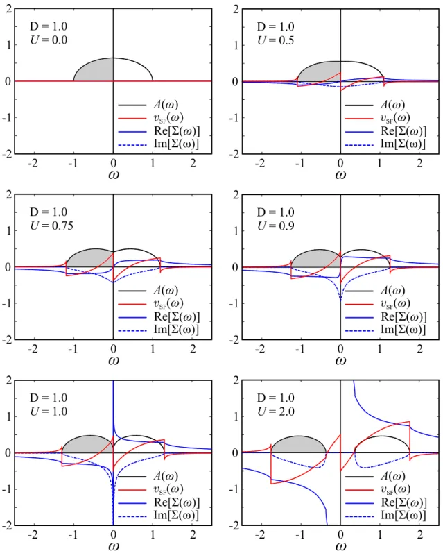
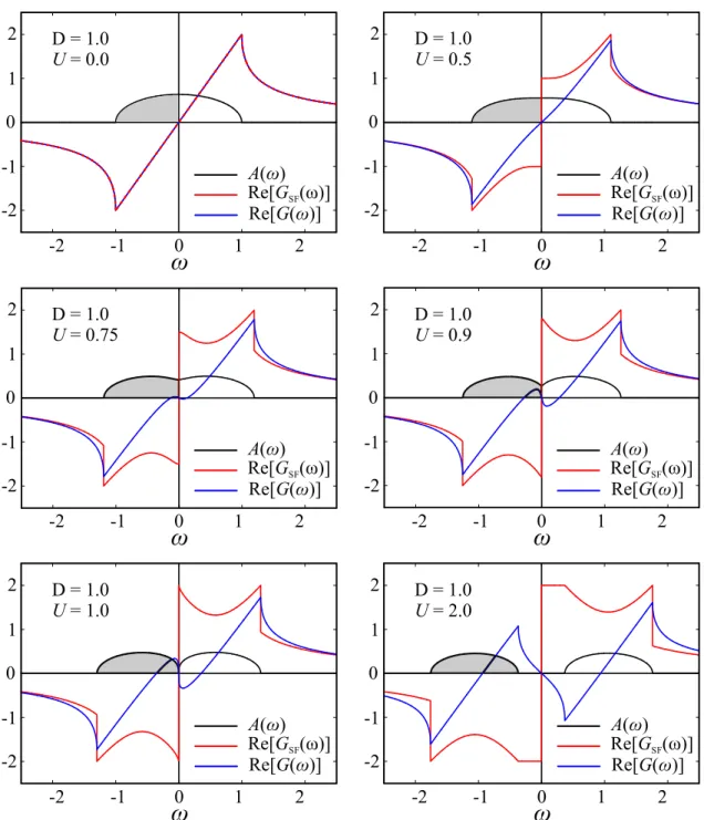
The first system we consider is the Bethe lattice with infinite coordination number. It de-scribes the Mott metal–insulator transition via the divergence of the imaginary part of the self energy, which is a purely frequency–dependent complex number. The challenge is therefore to describe the same transition via a real spectral potential, whose imaginary part, by definition, is always zero. In a second example we treat the symmetric Hubbard dimer, in which the self energy, besides being complex, is also non–local. As a consequence, the task of the spectral potential is doubled. Finally, we move to continuous system by considering the homogeneous electron gas (HEG), with a purely non–local self energy (the Heyd–Scuseria–Ernzerhof HSE06 one [12]). The challenge is transforming the non–locality of the self energy into the frequency dependence of the spectral potential.

However, this method is efficient if it does not require the knowledge of the self energy. Therefore, we propose a second shortcut (part III), which is pretty general and is inspired by the local density approximation (LDA) to the Kohn–Sham potential of DFT.

The strategy consists in evaluating the unknown quantity (the spectral potential) in a model system, and then import it in the auxiliary system through a suitable connector, that is a pre-scription that explains how to use the model system result in the original system.

I explain the general idea of this approach in chapter 5 and I apply it to the study of the asymmetric Hubbard model in chapter 6.

The real challenge, however, is treating realistic materials within this method. To this aim we consider the homogeneous electron gas as a model system, like in LDA. The spectral po-tential is evaluated there for a wide range of densities, and then imported each time a different material is studied. For this task, we propose a very simple connector based on local quantities only, hence the name dynamical local connector approximation (dynLCA) for this approach. The results for four prototypical materials, sodium, aluminum, silicon, and solid argon, are presented in chapter 7.

Note that the connector approach has a further practical advantage: in fact, the self energy is used just once in the model system only. Once the latter is solved and the results are stored2 for many values of densities, nobody will ever repeat the calculation in the model, nor will he/she perform a self energy calculation in the real material. One can completely abandon the

(19)

PREFACE

self energy, which is complex–valued and non–local, hence computationally heavy. At the same time, one does not have to build it for every different system; only the local quantities present in the connector are needed, and these can be obtained through a simple DFT calculation.

Besides the theoretical insight that it offers, this approach results in a drastic reduction of the computational cost. Therefore, it is particularly well suited for studying the properties of a large number of materials (material design), in which the use of a non–local self energy is usually the most time–consuming part. On the one hand, indeed, a local and real potential is computationally lighter. On the other, this method disentangles general properties due to the electron–electron interaction (accounted for by the calculation in the homogeneous electron gas) from specific properties of the material, that enter the form of the connector.

As I will show in this thesis, it is not easy to design a connector which is generally valid, and more work will have to be done. However, the results of this thesis are meant to show that this is a promising way to go, to answer some open questions and to open new ones.

(20)

Part I

Background

I needed to believe in a tale – however unlikely – which placed the events of this most terrible day in a sensible order. RICHARDZIMLER, The Last Kabbalist of Lisbon

La matière ne va pas jusqu’au bout, et l’isolement n’est jamais complet.

Si la science va jusqu’au bout et isole complètement, c’est pour la commodité de l’étude.1 HENRY–LOUISBERGSON, L’évolution créatrice

Though wisdom is common, the many live as if they had a wisdom of their own.

HERACLITUS, Fragments

1_{Matter does not go to the end, and the isolation is never complete. If science does go to the end and isolate}

(21)

(22)

Chapter

1

The experimental starting point

The aim of this thesis is to develop an efficient method for the description of observables re-lated to the electronic structure of matter. To validate the approach, we will benchmark it with the existing state–of–the–art theories. Therefore, we will not directly face the comparison with experiments. However, the connection with the experimental world is still of primary impor-tance, as it can guide us on choosing which quantities are important to reproduce theoretically. All the chapters that follow will focus on one particular measurable quantity, the spectral function. This is a key quantity for the interpretation of different crucial experiments, which are based on phenomena that have marked the development of quantum theory itself: the photoelectric effect and quantum tunnelling.

Indeed, the diagonal of the spectral function in real space is the fundamental observable for describing scanning tunnelling spectroscopy. Its diagonal in reciprocal space is the cornerstone of angle resolved photoemission spectroscopy. Finally its trace, which is basis independent, is the many–body quantity that is needed for reproducing photoemission and inverse photoemis-sion experiments.

Tunnelling spectroscopy is essentially a surface–sensitive technique. Also photoemission and its variants, according to the photon energy, are sensitive to the surface. However, they are extremely useful for investigating also the bulk properties of a system. In this thesis we con-centrate on the bulk, and photoemission will therefore be our primary reference experiment.

1.1 Photoemission spectroscopy

Photoemission experiments are the modern times development of some famous investiga-tions performed by Hertz in 1887, who observed what became known as photoelectric effect: under particular circumstances, a beam of monochromatic light is able to knock out electrons, thus called photoelectrons, from a solid. The quantum theoretical explanation [13] of this effect earned Einstein his Nobel prize: in an independent–particle picture (see fig. 1.1), a photon of frequencyω/2π is absorbed by one of the electrons of the material, with initial energy −εB− φ,

whereφ is the work function (energy needed to eject an electron from the highest occupied level, namely, in a metal, the vacuum minus the Fermi energy) andεB> 0 is the binding energy

of the electron, measured with respect to the Fermi energyµ. If the energy gain ħω is suffi-ciently large, that is if ħω > εB+ φ, the electron escapes the material into the vacuum, with

positive kinetic energyεk= ħω − φ − εB and momentum ħk, and is then collected by an

anal-yser.

This effect is at the basis of PhotoEmission Spectroscopy (PES), whose goal is to determine the energy levels of electrons in materials. Since conservation of energy states that −εB= εk−

(23)

1.1. PHOTOEMISSION CHAPTER 1. THE EXPERIMENTAL STARTING POINT

μ

φ

ﬁlled

states

empty

states

hω

ε

k

μ-ε

B

ε

k

μ

E

ﬁlled

states

empty

states

hω

μ+ε

B

ε

k

0

0 PES

IPES

Figure 1.1: Photoemission (PES) and inverse photoemission (IPES) processes schematically, in an independent particle picture. The wavy red arrow indi-cates a photon of energy ħω that enters the sample in PES (and exits in IPES); after the interaction, the sample is left with a hole, indicated by the white cir-cle, and N − 1 electrons (N + 1 in IPES), indicated by the blue spheres. The photoemitted electron (incoming electron in IPES) has energyεk. As it is ev-ident from this picture, PES probes the occupied states, while IPES the empty ones.

ħω + φ, and since εk is measured by a detector, ħω is chosen by the experimentalist and φ can be known, the electron binding energy can be determined from the kinetic energy of the photoelectron released in the vacuum.

Plotting the intensity of the signal, which is proportional to the number of photoelectrons, as a function of the binding energy, one obtains an extremely rich spectrum, where a series of distinct features reflects the different electronic energy states allowed in the material.

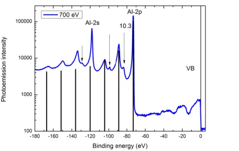
To make the discussion concrete, I will refer to a particular experiment in which I have taken part. It is an angle resolved photoemission experiment (ARPES, see below) on bulk aluminum, performed at the PEARL beamline of the Swiss Light Source (SLS1). The aim was collecting experimental data on the electronic structure of aluminum, and use a theoretical approach (the cumulant expansion) to describe them. An overview of the measured angle–integrated photoemission intensity as a function of the binding energy is shown in fig. 1.2, in logarithmic scale.

The most evident isolated sharp peaks are a signature of very localized core states, where electrons stick close to nuclei in an atomic–like way; their binding energies do not differ that much from the corresponding isolated–atom energies, hence they are used as evidences of the presence of a particular element in the sample (ESCA: electron spectroscopy for chemical anal-ysis [14]). In particular, in fig. 1.2, the most prominent peaks can be identified with the 2s and 2p atomic states. The line coming from the 1s state is at even lower energy and it is not shown. More complex to interpret is the region of the spectrum close to the vacuum level, the va-lence band. The ARPES spectrum in the vava-lence region at the k–pointΓ is shown in fig. 1.3.

In this region, more energetic, less bound electrons are allowed to explore the lattice struc-ture of the solid, exhibiting a stronger itinerant nastruc-ture. The discrete atomic–like energy levels

1_{https://www.psi.ch/sls/}

(24)

CHAPTER 1. THE EXPERIMENTAL STARTING POINT 1.1. PHOTOEMISSION

Figure 1.2: Angle integrated X–ray (ħω = 700eV ) photoemission data for alu-minum. Intensity (in logarithmic scale) of the photoemitted electrons as a function of the binding energy, in eV. The core levels 2p and 2s yield very sharp peaks in the signal, together with their plasmons. The valence band is, on the contrary, less pronounced; however, it is possible to distinguish, by the Fermi level, the quasiparticle with the characteristic ∼pω shape, that creates its own plasmons at lower binding energy (Experiment performed in collabora-tion, at SLS; figure from ref. [15]).

(3s and 3p in the case of aluminum) merge into a continuous distribution of energy in which electrons are allowed to dwell, the Bloch bands. In certain cases (Fermi liquids) the band pic-ture is enough to catch the main part of valence spectrum. This is the case when a prominent peak of finite width appears, the one at ∼ –10 eV in fig. 1.3 (see also fig. 1.4). It can still be interpreted as the fingerprint of the propagation of one single electron. However, its motion is now affected by the dynamical polarization of the medium: as one electron moves, the others are repelled and a Coulomb hole in the electron probability distribution surrounds the propa-gating electron. The interaction of the electron with the Coulomb hole slows it down and thus decreases its kinetic energy once it is ejected. In particular, from the relation −εB= εk−ħω+φ,

such a photoelectron will appear red–shifted with respect to the single–particle state to which it corresponds.

The higher the number of processes by which the electron can be decelerated, the wider the peak in the resulting spectrum. The width of the peak is thus interpreted as the inverse lifetime of the electron–plus–Coulomb–hole entity. The latter is called quasiparticle as long as it still exhibits a particle–like behaviour, namely as long as it can be thought of as a dressed particle with renormalized energy and mass. Quasiparticles, see fig. 1.4, get sharper and sharper as they approach the Fermi level, as the possibilities of decaying into non–coherent features is reduced by the kinematics of the process; on the contrary, well inside the Fermi sea (but still in the valence region), their lifetime is smaller and one does not see, nor one does talk about, quasiparticles there.

Bloch electrons in the valence band are an extraordinary source of other non–trivial many– body effects. One of these explains the series of smaller features that appear to the left of each

(25)

Figure 1.3: Angle resolved X–ray (ħω = 1100eV ) photoemission experiment on aluminum, at theΓ point. Intensity (in linear scale) of the photoemitted electrons as a function of the binding energy, in eV. (from ref. [15]).

most prominent peak in fig. 1.2. In fact, together with their neutralizing ions, valence electrons generate a plasma–like medium in which quasiparticles (core and valence) propagate. This medium, which is quantized and originally in its ground state, can take part in the photoemis-sion process by subtracting from the outgoing electron part of its energy, ħωP. As the medium

gets excited by one additional plasmon, the photoelectron is emitted with a lower kinetic en-ergy, resulting in a smaller peak to the left of the quasiparticle, called satellite (see for example in fig. 1.2 the feature at around –20 eV). With lower probability, the medium can also take twice the energy it needs to get excited, 2ħωP: it thus goes to a higher excited state, consisting of two

plasmons, and another satellite will show up in the photoemission spectrum, to the left of the previous one (the feature at ∼ –35 eV in the aluminum spectrum). And so on and so forth with lower and lower probability.

These series of satellites, smaller and smaller as they depart from their quasiparticle, show up to the left of each prominent peak of the photoemission spectrum, in the valence as in the core region. They are not energy levels in the one–particle sense, but they are a clear bench-mark of the collective behaviour of the electronic system [1], and they require a full many–body treatment to be theoretically reproduced.

Depending on the system, other mechanisms of energy–loss are possible [16], each resulting in other satellites in the photoemission spectrum.

Furthermore, in a photoemission experiment, other peaks can show up: they are the conse-quences of additional events like multiple scattering of the photoelectron before escaping the surface, or filling of the photohole left behind. Secondary processes like inelastically scattered electrons or results of “cascade” processes add up in the incoherent background which grows to the left (smaller kinetic energy of the photoelectron) of the most prominent features.

Finally, all spectroscopy techniques that involve electrons are highly surface sensitive. In particular, for kinetic energy of the photoelectron (which is determined by the photon energy and the binding energy range of interest) ranging from 100to 103eV, the corresponding electron inelastic mean free pathλeis 4÷40 Å [17], a few lattice constants inside the material. Therefore,

in general, the measured electrons stem from a region quite close to the surface. If one wants to probe the bulk, the surface must be as clean and as bulk–like as possible. Still, it will influence

(26)

CHAPTER 1. THE EXPERIMENTAL STARTING POINT 1.1. PHOTOEMISSION

the spectra. As an example, in fig. 1.3, the big shoulder at the right onset of the spectrum, at smaller binding energy than the quasiparticle, can indeed be interpreted as a non–dispersing surface contribution.

The qualitative picture I have just sketched shows how large is the possible number of effects that can occur in a photoemission experiment. To describe at least some of them, a reliable and efficient theory is needed.

1.1.1 The photoemission process

The standard approach to deal with the photoemission process from a many–body point of view simplifies the single photoemission event into the succession of three independent steps (three–step model [18]): an electron is excited by a photon in the solid, it propagates to the surface and it finally leaves the surface into the vacuum. Each of these steps contributes to the final photocurrent (detected electrons per unit time): an effective mean free path and a transmission probability through the surface take into account the last two steps [19], while the intrinsic photoexcitation of the electron can be described by the transition rate wf i from the

ground state of the N –electron system |Ψ(N )₀ 〉 to an excited state |Ψ(N )_f 〉 – driven by a perturbing Hamiltonian ˆHint. This is given, to first order in ˆHint, by Fermi’s golden rule [20, 21]:

wf i= 2π ħ ¯ ¯ ¯〈Ψ (N ) f | ˆHint|Ψ (N ) 0 〉 ¯ ¯ ¯ 2 δ³E(N )_f − E₀(N )− ħω´. (1.1) The perturbing Hamiltonian describes the interaction of the system with the electromagnetic field (φ, A). The scalar potential φ(r ) can be set to zero by a gauge transformation. The vector potential is supposed to be small (linear response: A · A = 0) and not varying with space (dipole approximation: ∇ · A = 0). With these assumptions, the perturbing Hamiltonian can be written as ˆHint= −i_mceħA · ∇ [17].

To evaluate the matrix element in eq. (1.1), a further simplification is usually made, called the sudden approximation2: the photoemitted electron is treated as completely decoupled from the sample; this allows one to factorize the final state |Ψ(N )_f 〉 into an antisymmetrized product of a photoelectron in the vacuum ˆc_k†|0〉 and the (N − 1) electron system left behind in the excited state s, |Ψ(N −1)s 〉. The photocurrent Jk(ω) is given by the total transition rate. It is

the sum over all possible excited states s: Jk(ω) =2π ħ X s ¯ ¯ ¯〈Ψ (N −1) s | ˆckHˆint|Ψ(N )₀ 〉 ¯ ¯ ¯ 2 δ³ε0 k+ E(N −1)s − E0(N )− ħω ´ ,

where the difference E₀(N )− Es(N −1) can be interpreted as the energyεs of an electron in the

solid, measured from the Fermi energyµ, and ε0_k is the energy of the free photoelectron in vacuum. The perturbing Hamiltonian can be expanded on a complete set of single–particle wavefunctionsφl as ˆHint=Pl l0cˆ†_l∆l l0cˆ_l0, with3∆_{l l}0= 〈l | ˆH_int|l0〉. Assuming that the ground state

|Ψ(N )₀ 〉 doesn’t have any component along |k〉, which is too high in energy4, one obtains: 〈Ψ(N −1)s | ˆckHˆint|Ψ(N )₀ 〉 =

X

l

∆kl〈Ψ(N −1)s | ˆcl|Ψ(N )₀ 〉 ,

and the photocurrent becomes: Jk(ω) =2π ħ X l l0 ∆kl∆∗ kl0 ½ X s 〈Ψ (N −1) s | ˆcl|Ψ(N )0 〉 〈Ψ (N ) 0 | ˆc † l0|Ψ(N −1)s 〉 δ ¡ ε0 k− ħω − εs ¢ ¾ . (1.2)

2_{The sudden approximation is justified when the kinetic energy of the photoemitted electron is large, which is}

the case for highly energetic impinging photons (see [22] to go beyond).

3_{In particular, for ˆ}_H

int= −imceħA · ∇ and constant A, in the reciprocal space basis the representation is diagonal: ˆ

Hint=mceħA · P

kk ˆc†_kcˆkand∆kk0= δ_kk0_mceħA · k.

(27)

While the first factors of the formula contain the radiation–matter interaction through the ma-trix elements∆kl, the part in curly brackets involves properties of the system only, from the excitation energiesεs to the transition amplitudes 〈Ψ(N −1)s | ˆcl|Ψ(N )₀ 〉. Such a quantity, for

rea-sons that will become clear later, is called spectral function and will be the main character of this thesis: Al l0(ω) := X s 〈Ψ (N −1) s | ˆcl|Ψ(N )₀ 〉 〈Ψ₀(N )| ˆc_l†0|Ψ(N −1)s 〉 δ ³ ω −εs ħ ´ . (1.3)

With its help, the photocurrent becomes: Jk(ω) =2π ħ2 X l l0 ∆kl∆∗ kl0Al l0 Ã ε0 k ħ − ω ! . (1.4)

Finally, the matrix elements∆kl are evaluated in the basis l in which A is diagonal, and it is often assumed that∆kl= const := ∆. Thus one arrives at the final formula:

Jk(ω) =2π ħ2|∆| 2X l Al l Ã ε0 k ħ − ω ! (1.5)

namely the important result that the photocurrent is, to some multiplicative factors, the trace of the spectral function which, as it is well known, is independent of the particular basis {|l 〉}l.

Inverse photoemission (IPES) Strongly connected to photoemission is the specular process

of inverse photoemission, which can be considered its time–inverted counterpart, as initial and final states swap their roles. Free electrons are sent on the sample, where they occupy empty levels; as a result, photons are ejected and collected by an analyser (see fig. 1.1).

The excitation energies are here defined asεs= Es(N +1)−E0(N ), and the conservation of energy

states thatε0_k= ħω−φ+εs. By repeating the argument just above, the transition rate is still given

by eq. (1.4) provided that the spectral function is defined as: Al l0(ω) := X s 〈Ψ (N ) 0 | ˆcl|Ψ (N +1) s 〉 〈Ψ(N +1)s | ˆc†l0|Ψ (N ) 0 〉 δ ³ ω −εs ħ ´ . (1.6)

Note that, besides being specular in time, IPES is also complementary to PES in the sense that, in a single–particle picture, it probes the empty levels of the system, while PES explores the occupied ones. The two approaches together give a full picture of the one–particle excitations of an electronic system.

Independent particles Neglecting the electron–electron interaction, the many–body system

is equivalent to many one–body systems; the transition amplitudes in eq. (1.3) or (1.6) simplify to 〈Ψ(N −1)s | ˆcl|Ψ(N )₀ 〉 = δl s, and the spectral function becomes:

A0_{l l}0(ω) := δl l0δ ³ ω −εl ħ ´ (1.7) with corresponding photocurrent:

J0 k(ω) = 2π ħ |∆| 2X l δ¡ε0 k− εl− ħω¢ . (1.8)

This is a series of delta peaks (see fig. 1.4 (b)) that can approximate at best the quasiparticle peaks; finite lifetime effects and collective excitations like plasmons are completely ruled out in such a picture. This is why, although very powerful for describing several properties of a many–electron system, effective one–particle approaches cannot in general catch the whole photoemission spectrum, and a truly many–body theory comes into play.

(28)

CHAPTER 1. THE EXPERIMENTAL STARTING POINT 1.2. STS

Figure 1.4: Angle–resolved photoemission spetroscopy: (a) geometry of an ARPES experiment with specified emission direction (ϑ,ϕ); (b) momentum– resolved spectral function for a noninteracting electron system with a sin-gle energy band dispersing acrossµ; (c) the same spectra for an interacting Fermi–liquid system (adapted from ref. [23]).

1.1.2 Angle Resolved Photo Emission Spectroscopy (ARPES)

In the last decades, Angle Resolved Photo Emission Spectroscopy (ARPES) has become fea-sible: besides energy levels, also their dependence on the wavevector k is experimentally ac-cessible (see fig. 1.4). ARPES is an extremely useful technique for investigating the dispersion of valence states which, as already mentioned, present an important itinerant nature; in par-ticular, for Fermi liquids, the position of the main quasiparticle peak as a function of k is the measured band structure. Also the Fermi surface, as a mapping of the k–points with energyµ, is directly accessible by ARPES.

To interpret ARPES experiments, one has to relate the measured momentum (in vacuum) to the wave vector k inside the solid: crossing the surface, the parallel (to the surface) component of the photoelectron momentum is conserved, while the perpendicular is not, and different approaches are used to determine it [19]. Besides the conservation of energy that we imple-mented above, also the momentum conservation in the solid must be taken into account: since the photon carries a negligible momentum in most cases, only vertical transitions are allowed, and the momentum of the electron in the material can be modified by reciprocal lattice vec-tors G only. These vertical transitions between bands are determined by selection rules in the matrix elements. Finally, the photocurrent emitted in the direction k is proportional to the diagonal of the spectral function in k space [17, 19]:

Jk(ω) =2π ħ2|∆kk| 2_A Ã k,ε 0 k ħ − ω ! , (1.9)

where A (k,ω) ≡ Akk(ω). As in eq. (1.5), the squared dipole matrix element |∆kk|2= ¯

¯〈k| ˆH_int|k〉 ¯ ¯

2

contains the radiation–matter interaction (in particular the dependence on the photon energy), while the whole many–body effects are accounted for by the spectral function, as it is clear from its definition: A(k,ω) = (P s〈Ψ(N −1)s | ˆck|Ψ(N )0 〉 〈Ψ (N ) 0 | ˆc † k|Ψ (N −1) s 〉 δ(ω − εs) if εs= E₀(N )− E(N −1)s ≤ µ P s〈Ψ(N )0 | ˆck|Ψ (N +1) s 〉 〈Ψ(N +1)s | ˆc_k†|Ψ(N )0 〉 δ(ω − εs) if εs= E (N +1) s − E(N )0 ≥ µ (1.10)

consistent with eq. (1.3) and (1.6). The main difference with angle–integrated photoemission is that ARPES selects a particular basis for the spectral function, while in photoemission only the trace of it is needed. This is why, if one wants to reproduce the outcome of ARPES experi-ments, the k–resolved spectral function must be evaluated, while any basis is fine for integrated photoemission.

(29)

1.2. STS CHAPTER 1. THE EXPERIMENTAL STARTING POINT

μ

sample

ﬁlled

states

empty

states

μ-ε

B

E

_tip

μ

tip

μ

tip

+ε

_Btip

E

_sample

ﬁlled

states

empty

states

E

tip

μ

tip

V < 0

V > 0

0 μ

μ+ε

_B

0

Figure 1.5: Scanning Tunneling Spectroscopy schematically, in an indepen-dent particle picture, for negative (left) and positive (right) bias V . The grey box is the sample while the blue object is the probing tip. The process is anal-ogous to the one of fig. 1.1. Alternatively occupied (V < 0) and empty states (V > 0) of the sample are explored.

1.2 Scanning Tunnelling Spectroscopy (STS)

A completely different experimental technique is Scanning Tunnelling Spectroscopy (STS), a purely surface–sensitive method based on the tunnel effect. The principle is very simple: a conducting probing tip is moved closer and closer to the surface of the sample, till the many– body wavefunctions of sample and tip overlap: in such a situation, if a suitable bias V is applied between tip and sample, tunnelling of electrons through the vacuum between the two becomes possible; thus, a tunnelling currentJ (V ) can be measured.

As the tip moves around, by measuring the tunnelling current one can achieve a complete reconstruction and visualization of the surface with atomic resolution (∼ 10−1÷100Å), produc-ing a real atomic microscope (STM: scannproduc-ing tunnellproduc-ing microscope [24]). Furthermore, be-sides visualization ot single atoms [25], also the manipulation of them became feasible within this technique [26].

Although the physical principle on which they are based is different (tunnelling a barrier versus absorption of a photon), both in this technique and in photoemission electrons propa-gate and eventually are emitted (or absorbed) from the sample, see fig. 1.5. Therefore it is not surprising that, even though the matrix elements – that account for the experimental setups – are unrelated, both currents are proportional to the same intrinsic quantity, namely the spectral function. In particular, since here the tip probes locally the sample and only the least–bound electrons partecipate to the current, the local spectral function evaluated in a neighborhood of the chemical potential shows up [27, 28, 29, 30] (assuming for simplicity the sameµ for both electrodes): Jr(V ) =4πe ħ Z µ µ−eVdω|T | 2_ρ t(ω + eV )A(r ,r ,ω), (1.11)

whereρt(ω) is the density of states of the tip and T is a matrix element depending, e.g., on the

(30)

CHAPTER 1. THE EXPERIMENTAL STARTING POINT 1.2. STS

geometry of the tip and the applied voltage V . It is not surprising that the densities of states of the two electrodes enter the formula, as electrons can jump between tip and sample only if the two can alternatively provide and accept electrons. In particular, depending on the sign of the voltage, empty (V < 0) or occupied states (V > 0) of the sample are probed, as the tip grants or gains electrons.

The sample enters eq. (1.11) through the spectral function in real space, defined as:

A(r , r0,ω) = (P s〈Ψ(N −1)s | ˆψ(r )|Ψ(N )0 〉 〈Ψ (N ) 0 | ˆψ†(r0) |Ψ(N −1)s 〉 δ(ω − εs) ifεs= E₀(N )− Es(N −1)≤ µ P s〈Ψ(N )₀ | ˆψ(r )|Ψ(N +1)s 〉 〈Ψ(N +1)s | ˆψ†(r0) |Ψ(N )0 〉 δ(ω − εs) ifεs= E (N +1) s − E0(N )≥ µ (1.12) which can be derived from the generic Al l0(ω) of eq. (1.3) and (1.6) via standard basis

transfor-mation.

In this chapter I have introduced an important object, the spectral function Al l0(ω),

which appears as a fundamental and recurrent quantity when considering different experimental techniques:

1) its traceP

lAl l(ω), that can be expressed in any basis, is needed to interpret

pho-toemission and inverse phopho-toemission experiments;

2) written in the reciprocal space basis, A(k,ω) constitutes the intrinsic (in the sense of independent of the measurement procedure) part of ARPES spectra;

3) its diagonal in real space A(r , r ,ω) is directly probed in scanning tunnelling spec-troscopy.

The spectral function contains essential information on the electronic structure of the sample, as can be seen from its definition, eq. (1.3) and (1.6). The challenge is therefore to derive it in the most efficient way from an ab–initio theory, in which just electrons and nuclei are present and no further parameters are used. I will show in the next chapter the state–of–the–art theory for obtaining the spectral function, while in the following I will develop a more efficient approach to the same goal.

(31)

(32)

Chapter

2

The many–body problem

When Richard Feynman was asked which single knowledge had better survive a hypotheti-cal fatal cataclysm, he replied with the atomic theory [31]: “that all things are made of atoms – little particles that move around in perpetual motion, attracting each other when they are a little distance apart, but repelling upon being squeezed into one another”.

The challenge was to transmit “the most information in the fewest words”, just one sentence to pass on to the next generation of (surviving) creatures. Had he been granted with more room, he would have probably specify that atoms – despite their name – were not the fundamental lego–bricks of nature.

Since the beginning of the century, indeed, scientists [32] have been aware that atoms are composed of big, heavy nuclei surrounded by light, tiny and fast electrons: their overall charge neutrality is the reason for the stability of atoms themselves, while the interplay between neigh-boring nuclei and electrons results in the attraction–repulsion dance that builds up the whole chemistry.

Well, not quite: it would be unfair to treat both nuclei and electrons with the same honours. The former, massive as they are, are pretty lazy compared to the far more active electrons. The latter move, scatter, lose and gain energy while, in many cases, one may consider that the nuclei stand by and watch, still approximately in their original state.

However, their only presence on stage is fundamental. Nuclei modify the properties of space around them, begging electrons for staying close. According to the configuration they assume, plenty of different materials come out, each one with its own characteristics.

Interacting electrons wandering in a lattice of nuclei will be the main character of the play described in this thesis.

2.1 The system

From a physical point of view, we can say that whenever two different time scales arise, a shorter one associated with electrons and a (much) longer one for the nuclear degrees of free-dom, the nuclear motion can be considered as adiabatically frozen with respect to the elec-tronic one; in this case, an adiabatic decoupling of their description is not only feasible but valuable.

(33)

2.1. THE SYSTEM CHAPTER 2. THE MANY–BODY PROBLEM

2.1.1 The Born–Oppenheimer decoupling

Indeed, soon after the birth of modern quantum mechanics [33, 34, 35], Born and Oppen-heimer [36] showed how it was possible to deal with molecules by decoupling the slow nuclear motion from the fast electronic one. Assigning a wavefunction for independently describing each of them,Ψ for the electrons and Φ for the nuclei, the wavefunction of the coupled system can be, in some cases [37, 38], just the direct product of the two,Ψ · Φ.

Such a case occurs in particular in common solids, where massive1 nuclei slightly move2 and light electrons quickly adjust to the instantaneous configuration of the formers. Their “ac-climatization” can be described by an electronic Schrödinger equation in which the nuclei en-ter only as a fixed set of parameen-ters {R_α}:

· E{Rs α}− ˆHe(r1, .., rN) − X i ,α veN(|ri− Rα|) ¸ Ψ{Rα} s (r1, .., rN) = 0, (2.1)

where ˆHe(r1, .., rN) is the purely electronic Hamiltonian (see below) that depends only on the

positions {ri}_{i =1}N of the N electrons, veN(|ri− Rα|) is the Coulomb interaction between an

elec-tron in ri and a nucleus in RαandΨ{Rs α}(r1, .., rN) is the electronic wavefunction, describing

electrons in r1, .., rNwhen the nuclei are in {Rα}, with the multilabel s that specifies a complete

set of quantum numbers for the electronic system.

The role of the eigenvalue E{Rs α}is twofold: it is both the (output) total energy of the electron

system and an (input) effective electronic energy that, on a longer time scale, contributes in determining the actual configuration of the nuclei. It is called (adiabatic) potential energy sur-face, and it is nothing but an electronic glue [39] that adds up to the nuclear Coulomb repulsion to set the dynamics of the lattice.

Indeed, the slower nuclear relaxation process can be described by the following nuclear Schrödinger equation, in which the electrons enter only through the potential E{Rα}

s : h Et ot ρ,s − ˆHN({Rα}) − Es{Rα} i Φρ,s({Rα}) = 0, (2.2)

where ˆHN({Rα}) is the purely nuclear Hamiltonian,Φρ,s({Rα}) is the nuclear wavefunction and

Et ot

ρ,s is the total energy of the electrons plus nuclei system, withρ a set of quantum numbers

for the nuclear Hamiltonian3.

Eq. (2.2) is a clear statement of adiabatic separation. It says that the nuclear motion does not modify the electronic state s, that enters as a parameter. In particular, electrons stay in their ground state E_s=0{Rα}. The Born–Oppenheimer approximation breaks down when, on the 1_{Even for the lightest atom, Hydrogen, the ratio between the mass of the electron and the nucleus is}

approxi-mately 1/1836: the non–relativistic two–body problem can be separated into a center–of–mass that behaves like a free particle, of mass M = mp+ me∼ mp, plus an orbiting particle of massµ =

³ 1 me+ 1 mp ´−1 ∼ me: eventually, in the center–of–mass reference system, a fixed “quasi–proton” and an orbiting “quasi–electron”.

2_{In a classical picture, the third Newton’s law states that the Coulomb force that an electron exerts on a proton is}

the same as the one that that proton exerts on the electron; as a consequence, their (change in) momentum is the same, hence their velocity is controlled by the ratio between their masses.

3_{A common approximation to E}{R_α}

0 is the harmonic one, where the adiabatic electronic potential is

approxi-mated by a quadratic function of the nuclear displacements, i.e., E{R₀ α}≈P

α12Mω2¡Rα− R eq

α ¢2, with Req_α the equi-librium position of theα–th nucleus: the Hamiltonian in eq. (2.2) results in a sum of independent harmonic oscil-lators, i.e., free phonons; additional anharmonic contributions can be considered, resulting in interacting phonons. A related approach, well suited in particular for molecules, is the separation of the nuclear dynamics into a rota-tional, vibrational and translational motion, pushing even forward the adiabatic separation idea by observing that different energy scales (i.e., time scales) are involved in the three mentioned processes.

Finally, we mention the Lennard–Jones [40] and the Morse potential [41], used to parametrize the energy surface

E{Rα}.

(34)

CHAPTER 2. THE MANY–BODY PROBLEM 2.2. THE PROBLEM

contrary, there is an interplay between electronic states and lattice dynamics, that is when two different energy surfaces E{Rα}

s and E_s{R0 α}are so close to each other (eventually, they cross) that

the slow nuclear dynamics induces transitions between different electronic states.

To conclude, eq. (2.2) states that it is possible to include the dynamics of the nuclei, and hence have access to the full many–body wavefunction in the Born–Oppenheimer approxima-tionΨ{R_α}(r1, .., rN)·Φ({Rα}), once the potential energy surface, and therefore the dynamics of

the electrons, is at hand. The latter is controlled by eq. (2.1), the real bottleneck of the calcula-tion. It is towards this very equation that we will now, and for the rest of the thesis, turn. 2.1.2 The electronic system

In atomic units4, which we will use for the rest of this thesis, the Hamiltonian that enters eq. (2.1) reads: ˆ H = N X i =1 Ã ˆp_i2 2 + v ext_{( ˆ}_r i) ! +1 2 N X i 6=j =1 1 ¯ ¯rˆ_i− ˆr_j ¯ ¯ (2.3)

where we have replaced the nucleus–electron interaction veN(|ˆri− Rα|) with a more generic

external potential vext( ˆri). This is the most general Hamiltonian we will consider. It describes

any realistic material in which 1) relativistic effects can be neglected, 2) spin–dependent inter-actions can be ignored and 3) the Born–Oppenheimer approximation holds.

These three requirements apply to a wide range of real physical systems, and we will focus in particular on crystalline solids, where the number of electrons is huge, of the order of the Avo-gadro number N ∼ 1023, and the arrangements of nuclei {R_α} is regular, that is ∀α ∃(n1, n2, n3) ∈

Z3

|Rα= n1a1+ n2a2+ n3a3, with {ai}3_{i =1}primitive lattice vectors.

Furthermore, we will attach the innermost electrons, the core electrons, to their nuclei, freez-ing them together into a positively–charged ion structure. This is called the frozen–core ap-proximation, and is motivated by the fact that only the valence electrons (the outermost ones) significantly contribute to the interatomic interaction. Hence N will be the number of valence electrons only, and vext( ˆri) the potential felt by an electron in ri due to the presence of the

whole ion lattice. For the rest of the thesis, we will consider this lattice in a fixed configuration {Rα}, and we will drop the label {Rα} from the formulas.

Finally, the Hamiltonian (2.3) completely defines the system, but we need the wavefunction Ψ to have access to its physical properties: the wavefunction obeys the Schrödinger equation, eq. (2.1), that reads5:

ˆ

HΨs(r1, .., rN) = EsΨs(r1, .., rN) (2.4)

Finally, with eq. (2.4) and eq. (2.3):

“The underlying physical laws necessary for the mathematical theory of a large part of physics and the whole of chemistry are thus completely known, ...”

2.2 The problem

“... and the difficulty is only that the exact application of these laws leads to equations much too complicated to be soluble.” [42]

4_{By definition, me}_{= e}2_{= ħ = 4π²}

0= 1; as a consequence, the unit of length is the Bohr a0=_α1_mħc

ec2 = 0.529 Å,

and the unit of energy is the Hartree Eh= α2mec2= 27.2114 eV.

5_{Since the Hamiltonian (2.3) does not couple spin and position variables, the total wavefunction will be}

factor-ized into the product of its spatial and spin components. The latter is not relevant for this thesis, and it will be not explicitly mentioned.

(35)

2.2. THE PROBLEM CHAPTER 2. THE MANY–BODY PROBLEM

Believe it or not, despite the fact that the electronic many–body problem is completely and exactly defined, finding the wavefunctionΨs(r1, .., rN) remains a formidable task. The reasons

are mainly three:

1. The number N of electrons in a solid is huge. Take for instance the sample we used for the ARPES experiment that I mentioned in the previous chapter. It is a cylindric sample of aluminum, 5 mm of diameter and 1.5 mm of height. It weights less than 0.1 g, but it contains roughly 0.23 · 1023electrons.

Is this a large number? Walter Kohn [43] tried to answer this question from an optimistic perspective: if only we were to describe a molecule (or an atom!) of N ∼ 100 electrons, by replacing each continuous coordinate (r(i ))k ∈ (−∞; ∞) in the wavefunction by just

3 parameters (a very rough trade!), the total numbers of these would be something like ∼ 10150, to obtain an accuracy in energy of ∼ 1%! No way to handle such a number, nor even to imagine it!

But let’s stay positive and assume that some intelligent being whispers to us the solution. We start recording it, but still, needing at least two bits per parameter, we would quickly run out of atoms to store our N = 100 electrons solution, since the total number of atoms in the universe is estimated to be around 1080(the situation is not always that drastic: in many cases, symmetries can help – see later with Bloch’s theorem). This observation – that goes under the name of van Vleck catastrophe [44] – pushed Kohn to the following provocative statement [43]:

“In general the many–electron wave functionΨ(r1, .., rN) for a system of N

elec-trons is not a legitimate scientific concept, when N&103”.

2. The previous point would not be a big deal, if only electrons wouldn’t interact. But they do, giving a job to thousands of physicists and, more importantly, life to billions of com-pounds, molecules and, eventually, human beings.

The interaction between electrons prevents the separation of ˆH into a direct sum of one– particle hamiltonians ˆh(i ). In general, one cannot even resort to a nearest neighbours model: the Coulomb interaction is long–range, meaning that each electron interacts, al-though sometimes weakly, with everyone else (in our 0.1 g Al sample,1₂N (N − 1) interac-tions means approximately 1044couplings)!

3. The third reason why eq. (2.4) poses a problem is a conceptual issue: having access to the wavefunctionΨ is not our final goal.

The wavefunction is an intermediate object that completely describes (the knowledge we have of ) a system. It contains all the information that can be extracted from it. In order to obtain in practice a piece of this information, one has to evaluate, from the wave-function itself, some reduced, much reduced quantities with the properties of 1) being observables (in order to be compared with experiments) and 2) depending on just a few variables (in order to have a clear physical interpretation). The wavefunction itself is not one of these quantities, being a complex object whose interpretation is not even always unambiguous [45].

And struggling to build up a giant for finally picking up just a tiny pinch of it doesn’t seem the most promising strategy.

Bearing these three arguments in mind – too many variables, an inseparable Hamiltonian and eventually an answer containing too much information – one had better give up on the quest for the full wavefunctionΨ, solution of eq. (2.4), and turn to what really matters.

(36)

CHAPTER 2. THE MANY–BODY PROBLEM 2.3. OBSERVABLES

2.3 Observables

What really matters is essentially just a bunch of operators – each one depending on a few degrees of freedom – whose expectation values are closely related to what is actually measured. Being properties of the system, these expectation values are still functionals of the wave-function but, containing (much) less information thanΨs, we expect them to describe the

sys-tem from a reduced perspective only. On the other hand, their immediate meaning makes it easy(–ier) to speculate about their structure, and their relative small size makes them appeal-ing quantities to work with.

The total energy The total energy of a system in the state s is formally defined by rearranging

the Schrödinger equation (2.4) for the eigenvalue Es, which becomes a functional Es= Es[Ψs]

of the wavefunctionΨs:

Es=

Z

d3r1...d3rNΨ∗s(r1, ..., rN) ˆHΨs(r1, ..., rN) . (2.5)

In particular, the ground state total energy E0 plays a crucial role. First, even at room

tem-perature (∼ 20 °C), most of common materials are in their ground state: take for instance our favourite Al sample (rS= 2.07 a0); its free Fermi energy (the valence band width) isε0_F =

11.65 eV, while kBT ∼ 25 meV; that makes a ratio of kBT /²0_F ∼ 0.2% thermally–excited

elec-trons! Even perturbing the system, this is usually expected to finally relax to its ground state. Finally, in the Born Oppenheimer approximation, by minimizing E0= E{R₀ α}with respect to the

lattice positions {R_α}, one can have access to many structural properties of the system itself (lattice constant, stress tensor, ...).

In conclusion, having the total energy of a many–body system means a lot. So much that, simply by inspecting Es as a functional of the wavefunction, eq. (2.5), we will be able to

in-troduce some very fundamental quantities, through which we will eventually reformulate the many–body problem.

The density Probably one of the simplest observables is the electronic density n (r ). It

de-scribes the distribution of electrons in space when the system is described by the wavefunction Ψ (that can either be the ground state Ψ0or an excited stateΨs). Density is defined as the

num-ber of electrons per unit volume, namely n (r ) := _dd N3_r

¯ ¯

¯_r. It is directly related to the probability amplitude of finding an electron in r , and its functional form in terms of the antisymmetric many–body wavefunction is:

n (r ) = N Z

d3r2...d3rNΨ∗(r , r2, ..., rN)Ψ(r ,r2, ..., rN) , (2.6)

which is the expectation value on the stateΨ of the density operator ˆn (r ) := P_{i =1}N δ(r − ˆri)6.

This is quite a simple quantity, depending on just three continuous variables (and not 3N as the wavefunction), whose visualization is extremely human–friendly: everyone knows what “dense” means.

Besides being in itself a compact and clear object, the electronic density is also a funda-mental ingredient for the expectation value of the many–body Hamiltonian (2.3). Indeed, the classical (self–)interaction energy of a cloud of charged electrons with density n (r ) is a simple functional of the density:

EH= 1 2 Z d3r d3r0n(r )n(r 0₎ |r − r0_| . (2.7)

6_{The two definitions are completely equivalent provided the Pauli principle applies: if this is the case, summing}

over all but the first argument of |Ψ|2does not highlight this as a preferred variable. Otherwise, the proper definition would be n (r ) =P

iR d3r1...d3rNδ¡r − ri ¢

Ψ∗_(r₁_{, ..., r}

Systèmes auxiliaires pour les observables : approximation du connecteur dynamique locale pour les spectres d'addition et d'émission d'électrons

HAL Id: tel-01803435

https://pastel.archives-ouvertes.fr/tel-01803435

Systèmes auxiliaires pour les observables :

approximation du connecteur dynamique locale pour les

spectres d’addition et d’émission d’électrons

Marco Vanzini

To cite this version:

T

HÈSE DE

D

OCTORAT

PARIS–S

É

COLE

P

OLY TECHNIQUE

Marco V

ANZINI

Auxiliary systems for observables:

dynamical local connector approximation

for electron addition and removal spectra

Contents

Table of main symbols and conventions

Preface

Part I

Background

Chapter

1

The experimental starting point

1.1 Photoemission spectroscopy

μ

φ

ﬁlled

states

empty

states

hω

ε

μ-ε

ε

μ

E

ﬁlled

states

empty

states

hω

μ+ε

ε

0

0

PES

IPES

μ

ﬁlled

states

empty

states

μ-ε

E

μ

μ

+ε

E

ﬁlled

states

empty

states

E

μ

V < 0

V > 0

0

μ

μ+ε

0

1.2 Scanning Tunnelling Spectroscopy (STS)

Chapter

2