1
1
Enhancing Knowledge for Renewed Policies against
Poverty
Working Paper n° 27
Using an Asset Index to analyse
Governance in Vietnam
Marine Emorine, La Hai Anh, Yoann Lamballe,
Xavier Oudin
IRD - VASS
This project is funded by the European Union under the 7th Research Framework Programme (theme SSH) Grant agreement nr 290752. The views expressed in this press release do not necessarily reflect the views of the European Commission.
2
Abstract
Using the PAPI dataset to analyse the relation between governance issues and poverty, we need to have a variable to measure the living standard of citizens, are there are no questions on income and expenditures in this survey. We construct an asset index based on the ownership of different assets by households.
This paper details the methodology used to calculate the asset index, the questions raised and how they are solved, and the results, with some empirical analysis of wealth distribution based on the new asset index.
The main conclusion of this paper is that the asset index provides a rightful measurement for households’ wealth, which allows exploring the links between governance and poverty in Vietnam using the PAPI dataset. It considerably widens the scope of the survey by adding a key characteristic of the households that can be utilised for deeper analyses.
3
Content
1. The asset index ... 4
Concepts ... 4
Methodology ... 5
Interpretation ... 6
Asset index as another measure of wealth ... 6
Limits of the asset index ... 8
2. Application to PAPI 2012-2013 ... 11
PAPI dataset ... 11
Asset index construction ... 12
Variable description ... 12
Variable selection process ... 13
Weights ... Descriptive statistics ... 16
Asset ownership across population ... 16
Distribution of wealth ... 17
3. Empirical analysis of wealth distribution ... 19
Noticeable difference between the indexes calculated on household heads and non-household heads. ... Consistency of the index: comparative results using VHLSS 2010 ... 21
Conclusion ... 25
4
Introduction
Surveys on households’ living standards usually estimate income and expenditures of the households and of their members through a set of questions that allow calculating a monthly income and the amount of monthly expenditures. These variables are commonly used to measure income distribution, poverty and many other characteristics of the households related to their living standards. They are also used for a number of socio-economic analyses where it is important to differentiate the population by living standards.
When data on income and expenditures are not available, one of the solutions is to create a proxy to measure wealth across the population. This is possible when the dataset provides information on household’s characteristics related to living standards such as the ownership of assets. The approach consists in building an asset or wealth index that will classify individuals or households according to their possession of items.
This paper presents asset indices and the application we can make of it with the PAPI (Provincial Governance and Public Administration Performance Index) survey. PAPI surveys are implemented under the guidance of the Vietnamese Fatherland Front and of UNDP. They are utilised to measure the performance of governance in the provinces of Vietnam from the perspective of citizens.
The first section reviews the basic concepts of asset indices, their construction and methodological issues. The second section presents the PAPI dataset and then applies a step-by-step methodology to construct the appropriate index. The third section gives some results using the constructed asset index, and compares the index with other measures of wealth in the VHLSS.
1. The asset index
ConceptAn asset index provides a relative measure of wealth across the population based on the individual’s ownership of a range of assets. Assets indices are considered as an alternative measurement of wealth, which reveals to be remarkably useful when monetary indicators of wealth are not reported in the survey data. For instance, many studies use a wealth index with the Demographic & Health Surveys (DHS) that provide national panel data on health, education and other household characteristics (Shea and Johnson 2004), but no information on economic conditions. Asset indices are also used to analyse poverty or inequalities evolution (McKenzie 2005, Booysen et al. 2002; Filmer 2005, Sahn and Stifel 2003), to control for economic status in program evaluation (Rao and Ibanez 2005), to target public programs (Schady and Araujo 2008). The World Bank also uses asset indices as another measure to describe poverty and inequalities changes in the World Bank Development Reports (World Bank 2003, 2005, 2006, 2011).
Discussions and debates are running on the quality or performance of asset indices as a measure of wealth (Foreit and Schreiner 2011, Howe et al. 2009). In 2012, Filmer and Scott produced a study assessing the performance of asset indices in term of measurement of poverty. They
5
found poor correlation between per capita expenditures and asset indices in different countries: on average, 50% of the poorest quintile with per capita expenditures is also classified in the poorest quintile with asset indices. However, the rich-poor gap in social outcomes, such as education, health care, fertility, child mortality, and labour market, is not very sensitive to the way households are classified. Therefore, despite the re-rankings of households, asset indices can be used to explore social inequalities.
This result must not be considered as disappointing as it seems to be. The main idea to remember is that it should not be expected that asset indices are perfect proxies for per capita expenditures. The main reason for this is that both measures do not represent the same concept of wealth.
Asset indices can have several interpretations in term of wealth, depending on the assets used in the index. The most basic approach uses strictly durables goods in the index construction. Households, in this case, are classified according to their material living conditions. This measure differs from classical concepts of monetary poverty and is said to represent a type of “long-run” wealth (Filmer and Pritchett 2001). The idea is that households with the best economic conditions in the past were able to save or invest more resources, which they used to purchase more durable goods. Other variables can also be added into the index. Some studies employ characteristics of the dwellings or of the household head, education, health or occupation but then, the interpretation of the index changes and become a “multidimensional index of welfare”.
Methodology
Each household is classified by an index, Ai, which is a function of a set of variables aij, indicating their ownership of asset j:
Ai = f(aij) = f(ai1,..., aik) j=[1;k]
Individual asset index Ai will therefore be computed as the sum of “assets” (understand durables or other households’ characteristics) owned by the household, to which is associated a weight for each asset:
Ai = (v1 x ai1) + (v2 x ai2) + ... + (vk x aik)
Statistical methods to compute such index differ on weight attribution for each asset. Methods for weighting include attributing an equal weight to each asset, using the monetary value of the goods or using the inverse proportion of households that own the asset. Each of those methods has their advantages and limitations. For the first one, household wealth is viewed as the accumulation of assets. The attracting simplicity of this method is challenged by the naivety of the concept: an equal weight for each asset is arbitrary and non-realistic, as we cannot consider that all assets have the same meaning in term of wealth. The second method, on the contrary, appears to be a “more realistic” measure of wealth, and can be considered as a sort of proxy for the household patrimony. However, it requires heavy and detailed information on the purchase of each asset, their monetary value and a calculation of depreciation. As the price of assets can vary between regions and across the years, this information must be collected. Finally, the last method, based on the inverse proportion of households who own the asset, works on the basis that assets that are the most owned by the population should have the smaller weights (they
6
are easy to get) and assets almost not owned the highest weights because they are the hardest to reach. Here, one of the most important methodological limits is that not all assets have a linear relationship with wealth; some assets might increase with income until reaching a certain threshold.
Weighting methodologies have been improved since the introduction of the Principal Component Analysis (PCA) or the Multiple Correspondence analysis (MCA) in asset index construction. Both of those statistical techniques are used in many fields as a reduction information technique: socio-economics, but also computing or epidemiology, etc. The intuition for weighting is the same that using inverse proportion of households, but takes account of the correlation of ownership of each asset. The highest weight will be accorded to the asset mostly not owned by the population but correlated with the possession of other assets, so that only the richest households, able to purchase a lot of assets can afford to own this item.
Arguably, MCA is considered as a better methodology than PCA for asset index construction because the latter is less appropriate for the analysis of categorical variables than the former. Recently, an improved version of PCA on STATA, called Polychoric PCA, was introduced. It proposes to deal with both sorts of variables. The idea is to estimate unobserved continuous variables from each observed categorical variables of our analysis. However, even though this technique offers methodological advantages, it relies on complex estimations that obscure the analysis and the comprehension of the results.
Statistically, the relevance of the asset index will mainly depend on the choice of assets used in the index. Some assets may provide poor information on household’s wealth, especially if the majority of the population owns it. Some assets can be closely correlated to the location of infrastructure and so, create a bias over-representing a region or rural households among the poor. Finally, some goods may have an ambiguous meaning across the whole population, e.g. can be owned for different reasons across groups of population. For instance, a radio can either be the primary source of information for poor people (denoting a sign of poverty) or either owned for leisure for middle or upper class. They can also be cases of group preferences, where assets are owned by a subset of population, because of cultural reason or different regional preferences.
Using the asset index must follow a robust and complete methodology. First, the concept of wealth that is approximate must be defined. Depending on this and the context of analysis (the population and the focus of interest), the variables included in the index must be carefully selected, with arguments on the process of selection. Then, the rightful statistical method must be employed. The results raised by the asset index must be confirmed by the relevance of the weights associated to each asset and the coherence of the classification of the population.
Interpretation
Asset index as another measure of wealth
In the literature, asset indices are often used as proxies of expenditures or incomes. Their wide use in Demographic Surveys (Demographic Surveys and Health –DHS- mainly) comes from the fact that these surveys do not have any direct question on income and expenditures of
7 households.
A proxy is a variable, not meaningful in itself, but which has the property of being highly correlated with an unmeasured variable. Since that variable is unmeasured, the property of correlation is just an hypothesis that cannot be verified. This hypothesis can however be tested in other surveys which have both kinds of variables. Many tests of that kind have been done, and they give mitigated results. Tests on the correlation between asset indices and per capita expenditures have been proved to not be very strong, although it can be reinforced when controlled by other variables (Filmer and Scott 2012). It must be recalled that expenditures as a measurement of living standards is itself a proxy for income. In developing countries, the World Bank recommends to use per capita expenditures instead of income to measure wealth and determine the poverty line. The reason is that the questions on income are not reliable. Respondents tend to hide or underestimate their income, especially non-wage incomes (Haughton and Khandker 2009). The answers on assets ownership are supposed to be more reliable than the one on expenditures and the one on income. Questions on ownership of assets are much easier to answer and yield fewer errors (wrong declaration).
The use of per capita expenditures as a proxy for income is also subject to shortcomings (both variables do not measure exactly the same thing) and the correlation between the two, when tested, does not give excellent results (see section 3 for an application to Vietnam). Using expenditures as a proxy of income can lead to erroneous understanding of poverty in a country. In Thailand for example, the ratio decile 10/decile 1 was 15.8 when using expenditures and 82.1 when using the income from the same surveys. The poorest decile spent 2.15% of the total expenditures but earned only 0.54% of the total income. The richest decile spent 34% of the total expenditures and earned 44% of the total income1. Using expenditures to measure poverty and tackle distributional issues can lead here to an underestimation of poverty (headcount, severity, etc.), to a wrong vision of inequality, to the ignorance of one of the major problem of poverty, which is debt, and so, to maladjusted policies.
In particular, high incomes tend not to be well captured by sample surveys. Even in countries with a performing statistical system, declarative surveys on incomes are weak to assess the richest part of the population (tax returns, also subject to underreporting, are deemed to be better). In Vietnam for example, owning a car is still a privilege and can just be afford by the very rich part of the population. In PAPI 2012-2013, 6.25% of the own a car (among them, there are probably cars for commercial use). Those definitely represent the richest part of the population. In VHLSS 2010, the average income of the 5 highest percentile is 8 million VND (less than 400 USD) per month, while the price of a medium car is over 1 trillion dong. In other words, the income of the richest part of the population in Vietnam is likely to be largely underestimated. When the asset index is used as a proxy of expenditures (in DHS surveys for instance), it is in reality a proxy of a proxy. Even though asset indices do not correctly proxy expenditures, and less imperfectly income, it does not mean that they are a bad measurement of wealth. It should
1 Data for year 1999 (the latest year where comparison is feasible), WIIC2 database of the World Institute
for Development Economics Research, University of the United Nations (UNU-WIDER)
8
not be claimed that they can replace expenditures or even income but more correctly understood that asset indices represent a different measurement of living standards.
Asset indices do not measure the same wealth as income and expenditures. In a way, it can be said that they capture another dimension of the living standards and, for the worse-off, of poverty. Being poor would not mean being under a certain threshold of monetary income, but being unable to afford a minimum of assets which are widely considered as necessary or desirable. In that sense, it is a measurement of patrimony2.
The asset index, when constructed using MCA technique as it is the case here, can be understood as a measure of distinction (in the sense of Bourdieu3). The hypothesis is than wealthier households acquire some items that poorer households cannot afford. The MCA will oppose those who own a computer and air conditioned to those who own a bicycle as the only mean of transportation.
The asset index may reflect a vision of inequality closer to the one felt by the citizens. In Vietnam, there is a feeling of growing inequality perceived by the population which is not corroborated by the statistics (the Gini index as computed in VHLSS surveys from 2002 to 2008 and based of the distribution of expenditures does not increase). .
This may be an explanation of the gap between the perception of citizens and the statistics. Differences of ownership of assets are more evidently perceived by citizens. If you neighbour can buy a car but you cannot, you may feel that this is unfair more evidently than in a difference of monthly expenditures.
So, if the asset index is not a good proxy of expenditures, it is nevertheless a valuable indicator of living standard and is meaningful to measure poverty and inequality. It can be more relevant than expenditures and incomes to analyse poverty under certain angles. But it also has its limitations.
Limits of the asset index
As any other measurements of wealth, the asset index remains imperfect and one should be conscious of its limits and restrictions to avoid erroneous interpretation. In the context of the present study, we can list a number of limits and restrictions associated with the use of an asset index.
One of the main limitation of the index is that it asset index provides a relative measurement of wealth, i.e. it assesses households ownership of assets compared to the others. Therefore, the index has no meaning in absolute value. It has no concrete meaning and may not easily be understandable for wide audiences.
Moreover, no ratio can be made with it - for instance, is not possible to say that someone who has an asset index twice higher than somebody else is twice richer. It has limitation when assessing poverty and inequalities. It cannot be used for poverty headcount or to calculate poverty gap, poverty severity or standard measures of income inequality such as the Gini coefficient or the class of Atkinson inequality measure (Harttgen, K. and Vollmer, S. 2011).
2 Asset indices are more a measurement of patrimony when they include house and land property, which
is not the case her.
3
9
However, it can be used for regressions and comparison in term of average between large enough subpopulations.
Besides, as discussed earlier, the asset index does not measure income over a given period, but accumulated wealth. Thus, it cannot render for short term fluctuations or the impact of shocks on income.
Other measures of wealth such as per capita income or expenditures are, by definition scaled to the household size while asset indices are not. Therefore, in some countries, the poorest households according to the asset index are the smaller families while the poor according to expenditures are systematically in larger households. Moreover, the asset index calculated in the case of the PAPI survey will tend to overrate the wealth of the youngest (especially those from age 18 to 25) as they declare their assets as well as their parents’, which they don’t directly own if they are still accounted in their family’s household. In consequence, an asset for household heads only has also been generated in order to correct the effect of age. However, in some extent this version of the index is also limited by the fact that there is no variable to qualify the relation with the head; as spouse or husband of the head would have the same level of asset owning as their relative.
Importantly, one of the main features of the asset index it that it is based on the consumption pattern of the studied population. This has a certain number of implications. Consumption patterns evolve rapidly through time and, within a few years, an item only owned by some happy few may become a mass consumption item (mobile phones, computers…). It is the case of Vietnam, which had a rapid and uninterrupted economic growth in the last twenty years and where consumption patterns have drastically changed.
Although access to mass consumption is a sign of better living standards, the change in the ownership of assets does not allow a direct measurement of the growth in wealth of households (but the study of the change in the basket of durable goods can hold). It is noteworthy that similar problems arise with other measurements (notably per capita expenditures) on the long run.
The ownership of some assets may be related to regional specificities, dwelling in urban or rural areas and, more generally, be influenced by cultural factors. This makes it difficult to classify households with different patterns of consumption on the same scale. For instance, owning a buffalo can be a sign of wealth among farmers in the northern part of Vietnam, while not owning a buffalo in the South does not mean that farmers are worse off. This in turns means that the asset index is more likely to identify rich households as being urban because urban households have easier access to assets and a way of life more turned toward consumerism4. The literature indeed support those criticisms and show that the poor, according to asset indices, are more likely to be in rural areas than the poor according to expenditures (Boysen et al. 2005; Lindelow 2006; Filmer and Scott 20125), but this is not the case in Vietnam (see section 3). Finally, this implies that cross-countries comparisons using asset indices are not possible
4 This is also the case for expenditures (see below, section 3). 5
These studies refer mostly to African context. They also contain housing characteristics in the index, and this explains most of the overrepresentation of rural households among the poor.
10
unless they have a similar pattern of consumption and use the same questions in the surveys to build the index6. Nonetheless, relative comparisons considering the ranking of each household in term of wealth can be used.
Another difficulty to be considered is the choice of the items. The assets selected must be distinctive of the living standards of households (which is closely related to the context) and in sufficient number to allow a significant ranking of the households using adequate statistical techniques. In the same time, they must not be too specific of the consumption of a category of the population (owning a tractor for instance is useless for classifying non-farm households). Survey designers are not always conscious of this problem; they may include items not relevant for measuring the wealth of households, and miss important items. In Vietnam context, owning flushed toilets is a significant sign of well-being but PAPI do not question about it. More generally, there are no assets concerning the house in PAPI, ownership of a house or apartment first, and elements of standing of the home (roof, amenities…).
These last considerations point out a major shortcoming of the asset indices which is the choice of items to be used to build the index. The selection of items is first decided by the designer of the survey and second, defined by the analyst constructing the index, both being necessarily subjective. One can partly overcome this problem by selecting appropriately the items to be put in the asset index. This signifies gaining using knowledge on the pattern of consumption and the hierarchy of assets acquired and numerous variable tests (on total and sub-groups of the population) notably to drop the assets that do not explain the variance.
The relative importance of each assets put into the index is another debated issue. At first glance, putting on the same scale a car and a fan looks unrealistic. If the asset index is only the addition of assets, it is necessary to translate into values the different assets. However this can be difficult and insufficient, especially when the number of items of each asset is not asked. This is the case of the PAPI survey, which questions follow the model: “do you or your household own the following (a car, a motorbike…)?” (Yes/No answer) and not “how many of these items do you own?”. But, even knowing the exact number of items applying an average value is not satisfactory as the real value of one good depends on its quality, age or brand (a car for example). This asset weighting difficulty is solved when using MCA, which does not rely on the monetary value of the item. MCA has the main advantage to use the covariance of the ownership of each asset across the population to deserve a different weight to each asset. The technique will therefore recognized high-value assets such as the ones that are associated with the detention of other assets (the hypothesis being that richer household can afford to cumulate more goods) but also detained by a small part of the population (so that only the richest households can afford to have it). In this way, weighting assets is no longer under the
6
This is the case of the Demographic and Health Survey (World Bank). Several papers present cross-country comparisons using the asset index (see among others Sahn & Stifel 2000, Booysen et al. 2007). Po et al. (2012) have also attempted to calculate the value of assets owned in different countries, using relative prices (based on World Bank CPI database) to allow comparisons. The University of Nijmegen has also elaborated a comparable asset index for 93 low and middle income countries. There are a limited number of items, but housing characteristics and access to public services are taken in account in the calculation of the index (see http://ddw.ruhosting.nl/iwi/ and Smits and Steendijk 2012).
11 judgement of the analyst and become partial.
2. Application to PAPI 2012-2013
PAPI datasetThe data we use come from the Provincial Governance and Public Administration Performance Index (PAPI) dataset. PAPI is Vietnam’s first publically available dataset providing an evaluation of governance from the perspective of citizens. The survey was first piloted in three provinces in 2009. Since 2011, PAPI covers all 63 provinces in Vietnam with a sample of over 13000 individuals each year.
The PAPI survey assesses six dimensions of governance: participation at local levels; transparency; vertical accountability; control of corruption; public administrative procedures; public service delivery. The survey mainly focuses on individual’s perceptions of governance, so that the questions used in the survey reflect the opinion of the society7.
Our sample is an appending of the 2012 and 2013 samples, and accounts for 26,294 citizens. The combination is permitted due to the fact that from one year to the other, the characteristics of the households and other variables of interest do not change importantly and that the enumeration areas stay the same (apart from one case of provincial capital change and some villages that have been redrawn, all the subdivisions stay the same)8.
The reason why we append two samples is that it allows having bigger subsamples for some categories of the population (especially ethnic minorities) and brings more robust results. It increases the significance of the answers (concerning questions on perception which can be biased by the context of the survey, having a bigger sample and two different times of surveying can be considered as an advantage).
We have recalculated weights to fit the new sample, and also because the weights of the original dataset did not fit to make calculation at the national level (only at provincial level). The weights that we use are a combination of the PAPI sampling weight9 and a postweight adjustment by province, gender, age and locality calculated from the 2012 Labour Force Survey10. As the survey only selects the population of individual over 18, the weight will adjust the sample in consideration11.
Originally, PAPI has been created to construct provincial indices of governance, based on the six dimensions above. The idea of the initiative is to compare the performance of provinces in term of governance. The PAPI provincial index of governance is now widely used and commented. It
7
See UNDP in Vietnam website (http://papi.vn/en/about-papi.html). Reports and numerous articles based on the PAPI survey can be found in this website.
8
1326 duplicates (from 2013) were dropped (+10 with no age and 8 below 18).
9
Calculated with the information taken from J. Acuña-Alfaro J. & E.J Maleski, PAPI Sampling Memo (2014).
10 The Labour Force Survey in 2012 uses population projections based on the 2009 census, made by
General Statistics Office (GSO).
11
The sum of the weighted sample is equal to around 61 million individuals, which is close to the projection of LFS 2012, but not equal as some proportionality issues can’t be assessed: non-representation of rural areas in Da Nang & Hai Phong or other post-strata in some provinces in the sample.
12
has become a political tool to assess publicly the performances of provincial governments. Our focus of interest is different. We want to explore the links between governance and poverty and inequalities in Vietnam. We do not make any analysis at the provincial level and do not intend to calculate any provincial indicator.
PAPI provides information on the subjective economic situation of the household (how would you describe your economic situation now, 5 years before and in 5 years?) and indication on whether or not the household is on the poverty list. However, the survey does not provide any further information on the economic situation of the household and none based on objective methods. For this reason, socio-economic study of governance using PAPI dataset has been limited to aggregate geographical analysis, by inserting additional economic information on the province or the district. Our demarche aims at resolving this problem, by constructing an asset index applicable to PAPI datasets that provides a measure of wealth at household level.
Asset index construction
Variable description
PAPI 2012-2013 offers a list of 16 durables assets households were asked to possess or not. Basic statistics give an idea of the density of ownership of each item.
Table1: Asset ownership summarized statistics
Unweighted Weighted
Variable Obs Mean Obs Mean
Car 26260 6,3% 61 468 357 5,3% TV 26282 96,8% 61 498 972 95,0% Cable TV 26260 40,0% 61 449 954 32,8% Motorbike 26260 89,1% 61 501 542 86,6% Landline telephone 26258 37,3% 61 488 444 31,5% Mobile telephone 26273 91,5% 61 496 173 89,2% Fan 26281 93,4% 61 500 372 91,1% Air conditioner 26273 17,9% 61 499 487 14,8% Radio 26278 20,8% 61 483 891 21,5% Water pump 26273 56,3% 61 457 132 62,5% Fridge 26278 63,9% 61 500 412 59,4% Camera 26270 13,7% 61 485 361 12,8% Calculator 26269 38,9% 61 469 497 35,5% Buffalo 26261 11,9% 61 455 034 16,5% Bicycle 26278 64,4% 61 566 056 64,5% Computer 26258 36,9% 61 489 058 30,0% Source: PAPI 2012-2013
On the above table, the missing answers have been recoded so that each variable can only have two values, 0 or 1. This manipulation enables us to notice that, from the initial 26,294 citizens, some of them did not provide complete information on their ownership of assets. This can
13
create a bias because if a citizen was not able to answer to all of the questions concerning his ownership of assets, then his index will not be a reflection of its wealth. For this reason, we decided to drop the households that did not provide information on 4 or more assets ownership. The table also shows disparities between asset ownership across the total population: some assets are almost universally owned such as TVs, and some are almost not owned, such as cars.
In addition, some questions from PAPI 2012 & 2013 provide qualitative information on the household living conditions such as access to electricity, the quality of the road closest to the house or the main source of drinking water.
Variable selection process
From the variables cited above, we decided to employ the following methodology:
- First, in order to measure correctly the standard of living of the population concerned, the assets selected in the index must contain sufficient relevant information on people’s relative wealth. Therefore, we decided to focus only on the sufficiently discriminatory variables.
- Second, we limit publicly provided assets that might create a bias by over-representing the rural population in the poorest and categorize only the urban population as the richest. - Third, we exclude « ambiguous » variables, e.g., variables that can have a different meaning
between categories of population.
Following the first point, assets commonly owned by the whole population such as TVs, mobile phones or electric fans were dropped from our analysis because they do not give much information about relative wealth as most of the population owns it. Nearly all households have electricity; some cases show incoherence with asset ownership (some households supposedly without access to electricity use electric devices). For this reason, we decided not to consider this information in the asset index.
The second point brings into focus information on the quality of the road closest to the house and the main source of drinking water. There are two main problems employing quality of road in the asset index construction. First, there are no other survey results that indicate which types of road is a sign of wealth or poverty in Vietnam. Second, quality of roads cannot be directly correlated with standards of living, as rich households may also live in rural areas close to unpaved roads. On the other hand, drinking water source provides a good characterization of households living conditions, especially if the household has access to tap water at home. We decided to drop ‘proximity to a paved road’ but to keep ‘tap water at home’ as an additional dummy variable in our analysis.
Finally, the last point requires the highest attention. Differences in preferences might over-represent one good in one subcategory of population. One way to check for the overall and regional linearity of ownership of each asset is to use other data providing information on asset ownership and on standards of living. In PAPI 2012-2013, we consider that three durables asset might have an ambiguous meaning. First, bicycles can either be owned by middle and high classes for leisure, and be a sign of wealth or either be owned by the poorest not able to afford a car or a motorbike. To resolve this issue we created a variable for encircling the poor people,
14
i.e. those who only own a bicycle and no other means of locomotion. Second, we know from the PAPI survey that TV is the main source of information in Vietnam and is owned by more than 95% of the population. Therefore, radio can either be an inferior good for the remaining 5% of the population or either be a leisure good. As the meaning of this item is not clear across people, we decided not to use it in the analysis. Finally, the buffalo asset was dropped, because the variable is too discriminatory towards farmers and rural population. If buffalo was included in the calculation, the coefficient related to owning a buffalo would be negative, which would mean that individuals who own this asset will have an index that would be automatically reduced. Nevertheless owning a buffalo can be interpreted in two ways; it can mean that the owner is producing crops with lower value added compared to fruit-bearing arboriculture or mechanised agriculture, but it can also mean that a buffalo owner is wealthier than an farmer who doesn’t own any. Furthermore, there is a large disparity in term of buffalo ownership depending on the regions. In rural areas in the Northern Mountains and in the North of the Central Coast, the proportion of individuals owning buffalo reaches respectively 49.2% and 40.3%, while those proportions only reach 20.5 and 9.3% in the Central Highlands and the Mekong River Delta.
At the end of the selection process, the final basket is composed of 12 assets that households might own or not. We decide to employ Multiple Correspondence Analysis (MCA) to assign the appropriate weight to each item as this method deals better with dummy variables. We expected all assets to have a positive sign, except owning bicycles without any other means of locomotion that should signal poverty.
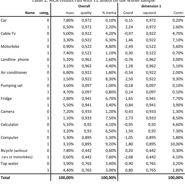
MCA results
The MCA approach uses covariance between the binary variables, so that the process can detect if an asset is positively or negatively correlated with the possession of others assets. From the result table below, all the variables have the expected sign. Owning a camera or an air conditioner are the highest signs of wealth across the sample while owning a bicycle (with no other means of transportation) or not owning a motorbike are the highest signs of poverty.
15
Table 2: MCA results run with 12 assets on the whole sample
Overall dimension 1
Name categ, mass quality % inertia Coord sqcoord Contri
Car 0 7,80% 0,972 0,10% -0,15 0,972 0,20% 1 0,50% 0,972 2,20% 2,24 0,972 2,60% Cable Tv 0 5,00% 0,922 4,20% -0,97 0,922 4,70% 1 3,30% 0,922 6,30% 1,46 0,922 7,10% Motorbike 0 0,90% 0,522 8,80% -2,49 0,522 5,60% 1 7,40% 0,522 1,10% 0,30 0,522 0,70% Landline phone 0 5,20% 0,962 2,60% -0,76 0,962 3,00% 1 3,10% 0,962 4,40% 1,28 0,962 5,10% Air conditioner 0 6,80% 0,922 1,80% -0,54 0,922 2,00% 1 1,50% 0,922 8,30% 2,50 0,922 9,30% Pumping set 0 3,60% 0,097 1,00% -0,18 0,097 0,10% 1 4,70% 0,097 0,80% 0,14 0,097 0,10% Fridge 0 2,80% 0,941 6,70% -1,65 0,941 7,70% 1 5,50% 0,941 3,40% 0,84 0,941 3,90% Camera 0 7,20% 0,933 1,20% -0,43 0,933 1,30% 1 1,10% 0,933 7,50% 2,73 0,933 8,50% Calculator 0 5,10% 0,92 4,10% -0,95 0,92 4,60% 1 3,20% 0,92 6,50% 1,50 0,92 7,30% Computer 0 5,30% 0,895 5,30% -1,05 0,895 5,80% 1 3,10% 0,895 9,20% 1,80 0,895 10,00% Bicycle (without 0 7,80% 0,442 0,60% 0,20 0,442 0,30% cars or motorbikes) 1 0,60% 0,442 7,60% -2,68 0,442 4,10% Tap water 0 3,90% 0,765 3,40% -0,90 0,765 3,20% 1 4,40% 0,765 3,00% 0,80 0,765 2,80% Total 100,00% 100,00% 100,00% Source: PAPI 2012-2013
16 Descriptive statistics
Asset ownership across population
Once built, we can use the Asset Index over the whole population (weighted) to categorize households into deciles or quintiles of wealth.
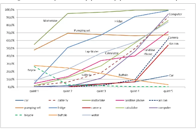
Figure 1: Ownership of durables by quintiles of population on the whole sample
Source: PAPI 2012-2013
The figure above outlines the path of consumption of different categories of goods:
- The relative lagged increase of cars, cameras and air-conditioner ownership with wealth indicates that those assets are “superior” (or luxury) goods that only the richest are able to buy.
- The steep slope of landline phones, cable TVs, calculators, computers, fridges and tap water means that those assets are “normal” (or basic) goods, which linearly increase with household wealth. Those are the goods in which the middle class gives priority to access.
- Pumping set and motorbikes are differentiated goods that are widely available and owned by quintiles of population at same proportion. The utility of those goods tend to decrease when households get richer, meaning that there are substitute goods more able to correspond to the wealthiest needs.
- Bicycle (when they are the only means of locomotion reported by the households) are inferior goods. The asset is accessible to all the population but only indispensable to the poorest ones.
17 Distribution of wealth
From the World Bank Poverty Assessment report (2012), we expect the poorest households in Vietnam to have a certain profile. Particularly, the poor in Vietnam accounts for an important part for farmers, and are primarily rural, concentrated in upland regions (notably North-West Mountains). Moreover, the share of poor must be more important among the ethnic minorities than for the Kinh majority. Finally, poor people are also characterized by low education attainment but have no correlation with age profile.
PAPI 2012 & 2013 provides information on these dimensions as well as some indications that can be used as statistical tests. Particularly, citizens were asked to evaluate the current economic situation of their household and had to say if they were in the poverty list (a Vietnamese government’s programme that supports poorest household).
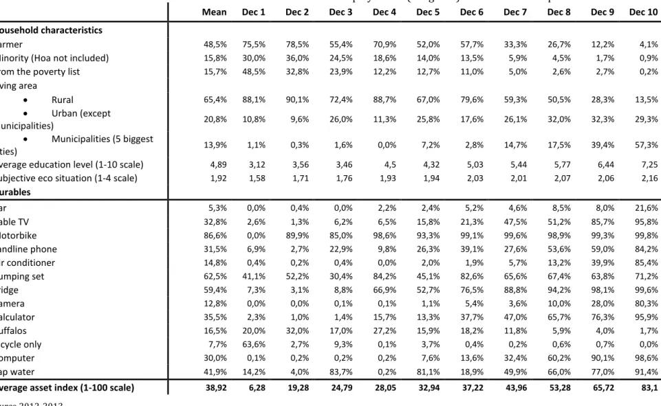
Basic household characteristics (table 3) by decile are consistent and confirm the robustness of the index constructed. The first two deciles group 63.8 of the households from the poverty list. When evaluating their economic situation, most of the people are not able to answer whether they consider their situation as good or bad. From the people considering their situation as bad or very bad, 55.8% are from the two poorest deciles, and conversely for the richest deciles where the proportion of those considering their situation as good is higher. The proportion of poor people is higher in the North than in the South, especially when only the first decile is considered. Finally, statistics show that the economic situation as measured by the asset index is strongly correlated with education and living areas:
- 71.8% of the people without education are found in the two poorest deciles. The average education level of the population is completed secondary school but the first five deciles of the Asset Index are below this level;
- 89.3% of the individuals in the two poorest deciles are live in rural areas while only 0.6% live in one of the top 5 cities of Vietnam. Moreover, 77.4% of the individuals of the first decile are farmers. In terms of asset ownership, the poor in rural areas are quite below the bottom population in urban areas.
18
Table 3: Households characteristics and asset ownership by decile (weighted) on the whole sample
Mean Dec 1 Dec 2 Dec 3 Dec 4 Dec 5 Dec 6 Dec 7 Dec 8 Dec 9 Dec 10
Household characteristics
Farmer 48,5% 75,5% 78,5% 55,4% 70,9% 52,0% 57,7% 33,3% 26,7% 12,2% 4,1%
Minority (Hoa not included) 15,8% 30,0% 36,0% 24,5% 18,6% 14,0% 13,5% 5,9% 4,5% 1,7% 0,9%
From the poverty list 15,7% 48,5% 32,8% 23,9% 12,2% 12,7% 11,0% 5,0% 2,6% 2,7% 0,2%
Living area Rural 65,4% 88,1% 90,1% 72,4% 88,7% 67,0% 79,6% 59,3% 50,5% 28,3% 13,5% Urban (except municipalities) 20,8% 10,8% 9,6% 26,0% 11,3% 25,8% 17,6% 26,1% 32,0% 32,3% 29,3% Municipalities (5 biggest cities) 13,9% 1,1% 0,3% 1,6% 0,0% 7,2% 2,8% 14,7% 17,5% 39,4% 57,3%
Average education level (1-10 scale) 4,89 3,12 3,56 3,46 4,5 4,32 5,03 5,44 5,77 6,44 7,25
Subjective eco situation (1-4 scale) 1,92 1,58 1,71 1,76 1,93 1,94 2,03 2,01 2,07 2,06 2,16
Durables Car 5,3% 0,0% 0,4% 0,0% 2,2% 2,4% 5,2% 4,6% 8,5% 8,0% 21,6% Cable TV 32,8% 2,6% 1,3% 6,2% 6,5% 15,8% 21,3% 47,5% 51,2% 85,7% 95,8% Motorbike 86,6% 0,0% 89,9% 85,0% 98,6% 93,3% 99,1% 99,6% 98,9% 99,3% 99,8% Landline phone 31,5% 6,9% 2,7% 22,9% 9,8% 26,3% 39,1% 27,6% 53,6% 59,0% 84,2% Air conditioner 14,8% 0,4% 0,2% 0,4% 0,0% 2,0% 1,9% 5,7% 13,2% 39,9% 85,4% Pumping set 62,5% 41,1% 52,2% 30,4% 84,2% 45,1% 82,6% 65,6% 67,4% 63,8% 71,2% Fridge 59,4% 7,3% 3,1% 8,8% 66,9% 52,7% 76,5% 88,8% 94,2% 98,1% 99,6% Camera 12,8% 0,0% 0,0% 0,1% 0,1% 1,1% 5,4% 3,6% 10,0% 28,0% 80,3% Calculator 35,5% 2,3% 1,0% 1,4% 15,7% 13,3% 37,7% 47,0% 65,7% 76,3% 95,9% Buffalos 16,5% 20,0% 32,0% 17,0% 27,2% 15,9% 18,2% 11,8% 5,9% 4,0% 1,7% Bicycle only 7,7% 63,6% 2,7% 9,3% 0,1% 3,7% 0,4% 0,2% 0,6% 0,7% 0,0% Computer 30,0% 0,1% 0,2% 0,2% 0,2% 7,6% 13,6% 32,4% 60,2% 90,1% 98,6% Tap water 41,9% 14,2% 4,0% 83,7% 0,2% 81,1% 18,9% 49,9% 66,0% 77,0% 91,4%
Average asset index (1-100 scale) 38,92 6,28 19,28 24,79 28,05 32,94 37,22 43,96 53,28 65,72 83,1 Source 2012-2013
19
3. Empirical analysis of wealth distribution
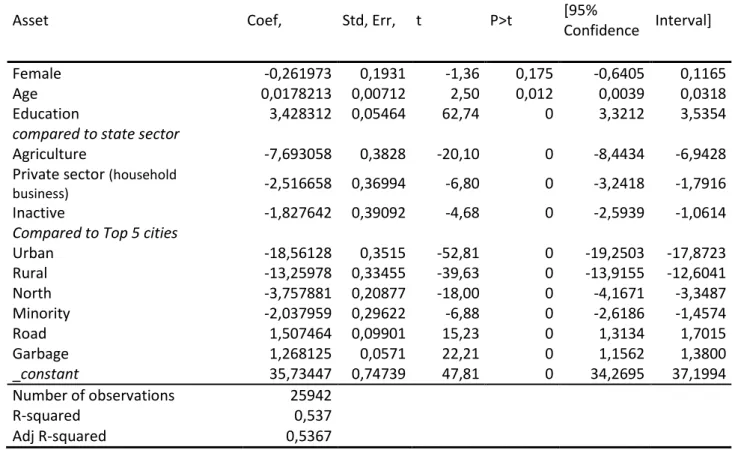
Our focus of interest primarily concerns being able to analyse poverty and inequalities in Vietnam using the PAPI 2012-2013 dataset. As a preliminarily analysis, we use a multivariate regression to assess the distribution of wealth across the Vietnamese population. The model uses Ordinary Least Square regression method on a set of general household characteristics. In table 4, results show that almost all explanatory variables of wealth are statistically significant and can explain more than 52% of the wealth distribution among the population sample. Among the highest coefficients, being a farmer has the strongest negative impact in term of wealth. This goes in line with similar statistical analysis using the VHLSS (Vietnam Households Living Standard Survey). The level of education is, as expected, highly determinant. Most importantly, all geographical variables, accounting for living in urban or rural area, in the North or South, and having access to a certain number of public infrastructures (road and water access quality, garbage picking) are all statistically significant and important factors of wealth distribution. This implies that geographical characteristics remains determinant to explain differences in wealth in Vietnam.
Table 4: Weighted OLS regression model using asset index (scale 0-100) on the whole population
Asset Coef, Std, Err, t P>t [95%
Confidence Interval]
Female -0,261973 0,1931 -1,36 0,175 -0,6405 0,1165
Age 0,0178213 0,00712 2,50 0,012 0,0039 0,0318
Education 3,428312 0,05464 62,74 0 3,3212 3,5354
compared to state sector
Agriculture -7,693058 0,3828 -20,10 0 -8,4434 -6,9428
Private sector (household
business) -2,516658 0,36994 -6,80 0 -3,2418 -1,7916
Inactive -1,827642 0,39092 -4,68 0 -2,5939 -1,0614
Compared to Top 5 cities
Urban -18,56128 0,3515 -52,81 0 -19,2503 -17,8723 Rural -13,25978 0,33455 -39,63 0 -13,9155 -12,6041 North -3,757881 0,20877 -18,00 0 -4,1671 -3,3487 Minority -2,037959 0,29622 -6,88 0 -2,6186 -1,4574 Road 1,507464 0,09901 15,23 0 1,3134 1,7015 Garbage 1,268125 0,0571 22,21 0 1,1562 1,3800 _constant 35,73447 0,74739 47,81 0 34,2695 37,1994 Number of observations 25942 R-squared 0,537 Adj R-squared 0,5367
Source: PAPI 2012-2013 Ethnic Minorities
Table 4 shows that ethnic minorities have in average a lower asset index scores in comparison to the Kinh (Viet) and Hoa. The inclusion of the Hoa group with the Kinh in the majority is fundamental, as they have the highest average asset index score compared to other groups and that those two groups are very close to each other. If we count Hoa as a minority in the dummy variable (minority
20
equal to 1), its coefficient becomes positive and statically significant; which would mean that in average Kinh have lower asset index scores in average than other groups.
Although the sample is big enough to differentiate between different ethnic groups, some are too small of unequally distributed in the enumeration areas. Moreover, there was no attempt to represent ethnic minority proportionally in the sample frame, and this variable was not used to stratify the sampling. The PAPI sampling strategy stresses the randomness of the subdivisions selection but not the representativeness of subpopulations (age, rural/urban and minority groups). Those gaps of representativeness are adjusted with the sampling weights and the postweights that make the sample representative at the level of the province and therefore at the level of the nation. But still, ethnic minorities are not properly distributed among the weighted sample. If the most important ethnic groups in term of population are well represented in the sample; the representativeness or non-representation of smaller groups is not guaranteed due to the sampling design and the limits of post weighting adjustments.
Another issue is the relation between assets and wealth among the different ethnic groups. Possession of goods cannot be only related to wealth but also to geographical, historical or cultural characteristics. As a matter of example, the Khmer people are the second minority group with the highest level of expenditure per capita if the Hoa and Ngai are excluded (both Chinese related groups very close to the Kinh) (MDRI 2014). Moreover, they are ranked first among the minority groups that have over 50 000 individuals (Hoa still excluded). However, in PAPI, they are among the lowest groups by average asset index score, and nearly 70% of them are concentrated in the three lowest deciles. In term of asset ownership in 2011 (permanent/semi-permanent houses, electricity, motorbikes, mobile phones, TV, fans, computers) Khmer households had low scores compared to the national average and average compared to other groups12. These contradictory results may be explained by consummation behaviours or cultural traits, but they reflect a limit of the assets index to represent wealth differences among subpopulations showing such diversity.
In our sample, the asset index of Kinh/Hoa is on 1.8 times higher than any of the other groups. However as minorities live mostly in rural (88%) this result must be relativized. In rural areas, the gap is smaller with Kinh and Hoa having a score in average 1.5 times higher than the other ethnic groups.
Activity sector and leadership position
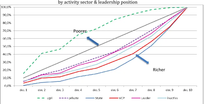
Two questions in the PAPI questionnaire deal with the job and sector of activity of the respondent (and the head of household, if he is not the respondent). We have recoded these variables which were originally not based on the international classification of industry. We consider here the distribution of the asset index by broad economic sector, namely the State sector (civil servants and workers of State owned companies), the private sector (employees of private firms, workers in household businesses and self-employed, the farmers (and fishermen) and finally the non-active people, most of them being retired.
The state sector has clearly the highest score in term of asset index compared to the other sectors, 79% of civil servants are in the 7th decile or over. The private sector is more homogeneously apportioned over the deciles, but still has a majority of individuals over the 5th decile (64.5%). Most of those in the private sector are in fact self-employed workers of heads of small household businesses, and can be assimilated to the informal sector. Farmers are mostly concentrated under the 5th decile (65%). The asset index score of the state sector is on average 2.1 than the average score of farmers. However 64.7% of those working in the state sector live in urban areas. If only rural
12
21
areas are considered, the average asset index score of civil servant is only 1.7 times higher than the one of farmers.
Moving to the leadership position (member of the Vietnam Communist Party (VCP), leader of a mass organisation or in the people’s comity), 68.1% of them are over the 5th decile. The most unequal distribution (towards the highest deciles) is found among the members of the Communist Party. The curve is not as bended towards the lower right as the civil servants but is following the same path. 68.6% of the members of the Communist Party are found over the 6th decile, 44.9% of them are among the 2 highest deciles. This can be explained by the fact that 23.6% of the individuals from the state sector are members of the party, and that 42.6% of the members of the VCP work (or used to work) in the state sector. Moreover there is a gap in term of membership rates between localities as 8.2% of individuals living in urban area are members of the party and only 3.9% of individuals living in rural areas are members.
Figure 2: Cumulative distribution (in %) over asset index deciles of individuals by activity sector & leadership position
Source: PAPI 2012-2013
Further analysis of poverty and inequalities should account for more sophisticated specifications as the present model might face some bias, notably regarding endogeneity and double causality issues. As said previously, asset ownership measures a kind of long run wealth, which is more resistant to economic shocks than income or expenditures measures. Therefore, it estimates a persistent form of poverty or wealth that might constraint household choices such as education and geographical mobility. Because of that, it is to be expected that the coefficient of the former variables might be underestimated. However, the regression above reaffirms the relevance of the asset index in the analysis of wealth, poverty or inequalities with PAPI data. This opens for deeper studies on local governance in Vietnam, which is the objective of the PAPI surveys. Some of the major findings concerning governance can be tested and verified, such as the impact of corruption on the poorest or the degree of participation and inclusion of the society according to economic status. It can be assessed which channels hinder the most the transmission of information to citizens, controlling by household economic situation. Finally, an analysis of inequalities can also be made by emphasizing which dimensions of governance disadvantage the poorest and which ones advantage the richest. In
Poorer
22
this regard, we expect high inequalities between rich and poor concerning governance, as most of the variables are based on people perceptions and perceived inequalities tend to be much higher than measured inequalities in Vietnam (World Bank, 2012).
Consistency of the index: comparative results using VHLSS 2010
In order to test the relevance of the asset index to estimate wealth in Vietnam, we proceed to a comparative analysis of PAPI 2012 with the 2010 Vietnam Household Living Standards Survey (VHLSS) results. The VHLSS is a nationally representative survey conducted by the General Statistics Office (GSO) of Vietnam that mirrors the World Bank's LSMS. The VHLSS, run every two years, are the main source of statistics and economic analyses concerning poverty headcount and income distribution in Vietnam.
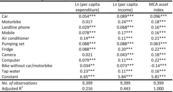
With regard to the criticisms addressed to asset indices as a rightful measure of wealth, we attempt to compare alternative approaches to welfare measurements, including income, expenditures and asset index by using VHLSS 2010. To measure the asset index, the basket of durable assets available in PAPI 2012 is applied. They consist of 11 assets: car, motorbike, landline phone, mobile phone, air conditioner, pumping set, fridge, camera, computer, bicycle (without car/motorbike) and tap water13. Estimated coefficients on this set of assets are statistically significant at one percent and have expected signs (except the bicycle variable) in both income and expenditure regressions, which are shown in Table 5. However, results differ on the power of explanation of this set of baskets for the two measures. As can be seen, the basket of assets explains only 22% of expenditures model but 44% of income model. It also appears that estimated coefficients in the MCA asset index model are closer to those in income model (table 4).
Table 5: expenditures, income and MCA index regressed by assets
Ln (per capita expenditure) Ln (per capita income) MCA asset index Car 0.054*** 0.089*** 0.096*** Motorbike 0.017 0.24*** 0.18*** Landline phone 0.029*** 0.068*** 0.16*** Mobile 0.078*** 0.17*** 0.16*** Air conditioner 0.14*** 0.11*** 0.21*** Pumping set 0.088*** 0.088*** 0.063*** Fridge 0.088*** 0.20*** 0.22*** Camera 0.021 0.043*** 0.18*** Computer 0.079*** 0.11*** 0.22***
Bike without car/motorbike 0.034** 0.073*** -0.14***
Tap water 0.23*** 0.11*** 0.16***
Constant 6.65*** 5.84*** 5.81***
No. of observations 9,399 9,399 9,399
Adjusted R2 0.216 0.443 1.000
Source: 2010 VHLSS
Note: (i) The un-centred variance inflation factors (VIF) < 2.30 (ii) * p ≤ 10%, ** p ≤ 5%, *** p ≤ 1%
(iii) The population weights are applied
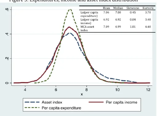
Furthermore, the distribution of asset index appears to be closer to that of per capita income compared to that of per capita expenditure. From Figure 2, we can see that the income variable
13 Cable TV, calculator and buffalo are not used to measure asset index with VHLSS 2010 because of
23
shows the most symmetric distribution with the median closest to the mean and the smallest values of skewness and kurtosis (closest to zero and three, respectively). Although better reflecting the income distribution, the MCA asset index skews to the right tail. This skewness reduces when adding household characteristics to measure MCA index.
Figure 3: Expenditures, income and asset index distribution
Source: 2010 VHLSS. Note: The population weights are applied
To assess how household rankings differ when applying the alternative approaches to measuring economic status, we use two methods to compare household rankings. The first compares the simple correlation of household rankings across the different measures. Beside income, expenditure and MCA asset index, two other measures are also implemented: (i) share weighted average, which uses the proportion of the population using each asset as weights; and (ii) count index, which simply takes the number of assets as its values. The second estimates the share of the population that is simultaneously ranked in the poorest quintile by different measures.
Table 6 shows the Spearman rank correlation between welfare indicators and log of per capita income/expenditure as well as the MCA asset index. The various measures yield statistically significantly related household rankings. From the table, we find that log of per capita expenditure is slightly less correlated to MCA asset index than to log of per capita household income or its predicted values (0.32 vs. 0.40 or 0.36). The same result is found among the rank correlation of log of per capita income with its predicted value and with MCA asset index (0.60 vs. 0.62). However, the correlation between MCA asset index and income approximately doubles that between MCA index and expenditure. In addition, the rank correlation among the various asset indices is very high. The correlation between the ranking derived from MCA and the other indices is typically greater than 0.85. Even predicted per capita expenditures/income is also highly related to the MCA asset index, almost three times higher than the correlation between income/expenditure and their predicted values.
24
Table 6: Spearman rank correlations Ln(Per capita expenditure) Ln(Per capita income) MCA asset index
Ln(per capita expenditure) 1 0.397 0.315
Ln(per capita income) 0.397 1 0.602
Predicted ln(per capita expenditure) 0.358 0.565 0.849
Predicted ln(per capita income) 0.324 0.615 0.972
MCA asset index 0.315 0.602 1
Matching score 0.287 0.544 0.869
Share weighted average 0.295 0.586 0.947
Count index 0.325 0.608 0.970
Source: VHLSS 2010. Notes: All tests reject H0 at one-percent significant level (H0: two variables are
independent).
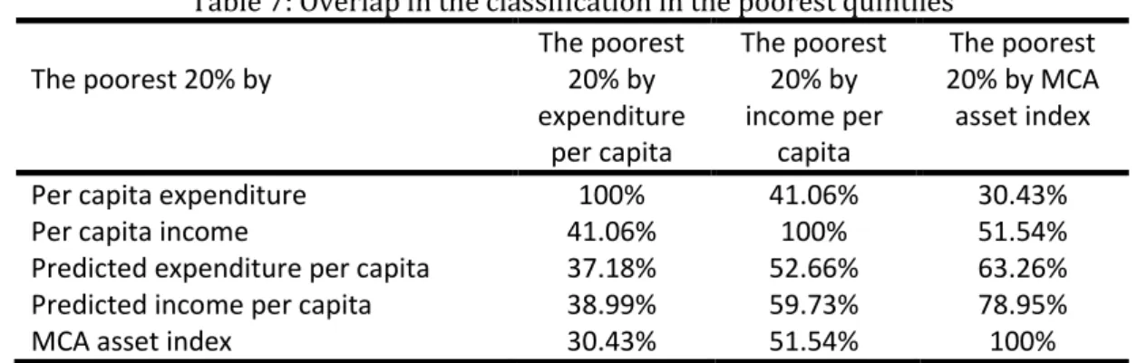
We also check the validity of asset indices in poverty issues. First, we check the overlap between the different poorest quintiles (table 7). Although only 30% of people in the poorest quintile by per capita expenditures are also categorized in the poorest quintile by the MCA asset index, this figure is also low for the lowest-quintile overlap between per capita expenditures and per capita income or its predicted values (37-41%). Similarly, 52% of people from the poorest quintile by per capita income is also classified in the poorest 20% by the MCA asset index and comparable to the overlap for per capita income and predicted values (53-60%). These figures are bigger in the case of overlapping MCA asset index with predicted expenditure (63%) or with predicted income (79%), even higher than the overlap for income/expenditure and their predicted values. This result again confirms that the asset index is better representative for per capita income rather than expenditure.
Table 7: Overlap in the classification in the poorest quintiles The poorest 20% by The poorest 20% by expenditure per capita The poorest 20% by income per capita The poorest 20% by MCA asset index
Per capita expenditure 100% 41.06% 30.43%
Per capita income 41.06% 100% 51.54%
Predicted expenditure per capita 37.18% 52.66% 63.26%
Predicted income per capita 38.99% 59.73% 78.95%
MCA asset index 30.43% 51.54% 100%
Source: VHLSS 2010
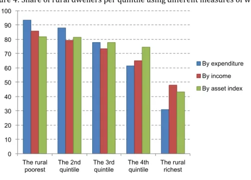
Second, we compare the distribution of five quintiles in urban and rural areas for expenditure, income and the asset index (figure 3). Being consistent among various measures, the share of rural population is larger among the poorer and smaller among the richer. However, there is a trend that less rural households are found among the poor if the asset index is used to classify the population. This goes against the empirical predictions saying that asset indexes tend to over-represent rural people among the poor (Filmer and Scott 2012). In our case, actually, rural inhabitants represent a highest share of the poor and a smaller share of the rich with expenditures than with other wealth measures.
This demarche clearly shows that the three alternative measures of wealth present different results in term of measure of wealth in Vietnam. Interestingly for our analysis, the asset index, based on the items in use in the PAPI survey, is better related to income than to expenditures. As the ownership of assets can be considered as an accumulated wealth, it is not surprising that the correlation is
25
better than with expenditures. But if incomes are subject to short term fluctuations, asset indices have, on the contrary, a strong inertia. Measuring wealth on a longer-run than other measures of wealth (as argued by Filmer and Pritchett 2001), it means that the asset index is more likely to capture long-run poverty.
Figure 4: Share of rural dwellers per quintile using different measures of wealth
Source: VHLSS 2010
Also, we found that asset indices do not over-represent the rural population among the poor but that expenditures do. In other words, when using expenditures, poor urban people in Vietnam are more likely to consume relatively more than poor rural people, and so, will be classified as richer than they are. One explanation is that, in the case of Vietnam, consumption expenditures might face some failures. For instance, people might have higher consumption in urban areas because goods are more expensive and life requires more expenditure. Those constrained expenses cannot be distinguished from non-constrained expenses, and so, will automatically lower the share of urban dwellers among the poor.
Conclusion
We have created a measure of wealth applicable to PAPI surveys data that considerably extends the use of the dataset and opens up for a microanalysis of the links between poverty and governance in Vietnam, not only at provincial or district levels, but also at national level.
This asset index is limited by the available information found in the PAPI survey. It could be improved if some additional questions were asked. More questions on housing could bring valuable information on households’ wellbeing. For instance, the ownership of flushed toilets is considered as a good indicator of living standards and is well correlated with income, according to some additional tests with the VLHSS 201014. More detailed information on the assets owned could also improve the quality of index. For instance, a distinction can be made between cars used for private purposes and commercial vehicles.
Another possible and easy to implement improvement is to ask about the number of items owned,
14
26
at least for some items (motorbike, buffalos…). This would not overload the questionnaire and would bring much more variance in the variables. Owning a motorbike is nearly universal in the country and so, is not much useful for the asset index. A household with three adults who owns only one motorbike is obviously poorer than an equivalent household who owns three motorbikes, but they are treated the same way in the present asset index. The index would be much more relevant if we knew the number of motorbikes detained by the household (it would then be weighted by the number of adults in the household).
On the other hand, it seems not suitable to ask the value of the items owned. It would considerably load the questionnaire and divert the interview from its objectives, without bringing reliable information. MCA remains the rightful methodology to assign the weight of each item.
Apart from the statistical recommendations, we also advocate more considerations for asset indices in the analysis of poverty and inequalities in Vietnam. It appears clearly that asset indices can capture a different form of poverty, more persistent and more structural than income or expenditures measures. This information may be useful for better targeted policies. Finally, the asset index is an interesting tool to assess inequalities in the country, closer to the population perception and hence, important for policy makers.
To conclude, we argue through this analysis that the asset index represents a rightful measure of wealth in the case of Vietnam, although results might differ from other analyses using traditional monetary measures of wealth. This legitimates its use with PAPI datasets. Furthermore, asset indices have comparative advantages for some specific targeting programs on the poor and rural households. Therefore, we believe that their use should be more considered in current socioeconomic analyses by researchers as well as by policy makers.
27
References
Acuña-Alfaro J. & E.J Maleski (2014). PAPI Sampling Memo, UNDP.
Booysen F., Van Der Berg S., Burger R., Von Maltitz M., Du Rand G. (2007), Using an asset index to assess trends in poverty in seven Sub-Saharan African countries.
Bourdieu P. (1979). La distinction. Critique sociale du jugement. Les Éditions de Minuit, Paris (English translation : (1984) Distinction. A Social Critique of the Judgement of Taste. Harvard University Press).
Deaton, A., & Zaidi, S. (2002). Guidelines for constructing consumption aggregates for welfare analysis (Living Standards Measurement Study Working Paper No. 135). Washington, DC: The World Bank.
Evans, D., & Miguel, T. (2007). Orphans and schooling in Africa: A longitudinal analysis. Demography, 44, 35–57.
Filmer D. and Scott K., (2012) Assessing Asset Indices. Demography, 49, 359–392.
Filmer, D. (2005). Fever and its treatment among the more and less poor in sub-Saharan Africa. Health Policy and Planning, 20, 337–346.
Filmer, D., & Pritchett, L. (2001). Estimating wealth effects without expenditure data—or tears: With an application to educational enrollments in states of India. Demography, 38, 115–132. Filmer, D., & Scott, K. (2012). Assessing asset indices. Demography, 49(1), 359-392.
Foreit KGF, Schreiner F. M. (2011). Comparing Alternative Measures of Poverty: Assets-Based Wealth Index vs. Expenditures-Based Poverty Score. Measure Evaluation PRH, WP-11-123.
Harttgen, K. and Vollmer, S. (2011). Inequality Decomposition without Income or Expenditure Data. Using an Asset Index to simulate Household Income. Human Development Research Paper 13, UNDP.
Haughton J. and Shahidur R. Khandker (2009). Handbook on Poverty and Inequality, the World Bank, Washington DC.
Howe LD, Hargreaves JR; Sabine G, Huttly SRA. (2009) Is the wealth index a proxy for consumption expenditure? A systematic review. J Epidem Commun Health. 2009;63:871-880.
Johnson D. and Abreu A., (2012). Johnston, D., & Abreu, A. (2013). Asset indices as a proxy for poverty measurement in African countries: A reassessment. Paper presented at the African Economic Development: Measuring Success and Failure, Simon Fraser University,
Vancouver, Canada. Retrieved from http://mortenjerven.com/conference-program-2013/ Lindelow, M. (2006). Sometimes more equal than others: How health inequalities depend on the
choice of welfare indicator. Health Economics, 15, 263–279.
McKenzie, D. (2005). Measuring inequality with asset indicators. Journal of Population Economics, 18,229–260.
MDRI (2014). 54 ethnic groups: why different, Mekong Development Research Institute, Hanoi. Po, June Y. T., Jocelyn E. Finlay, Mark B. Brewster, David Canning (2012). Estimating household
permanent income from ownership of physical assets. Center for Population & Development Studies, Harvard University.
Rao, V., & Ibanez, A. M. (2005). The social impact of social funds in Jamaica: A “participatory
econometric” analysis of targeting, collective action, and participation in community-driven development. Journal of Development Studies, 41, 788–838.
Sahn, D. E., & Stifel, D. C. (2000). Poverty comparisons over time and across countries in Africa. World Development, 28(12), 2123–2155],