THÈSE
En vue de l'obtention du
DOCTORAT DE L’UNIVERSITÉ DE TOULOUSE
Délivré par l’Universités Toulouse III Paul SabatierCotutelle internationale avec :
Université des Sciences de Hanoï
Ecole doctorale et discipline ou spécialité :
ED SDU2E: Océan, Atmosphère et Surfaces Continentales Unité de recherche :
Laboratoire d’Etudes en Géophysique et Océanographie Spatiales, Toulouse, France Directeur(s) de Thèse :
Patrick MARCHESIELLO, Sylvain OUILLON, Van Uu DINH Rapporteur(s):
Bruno BLANKE, Kim Dan NGUYEN, Thong NGUYEN
Présentée et soutenue par : Nguyet Minh NGUYEN
Le 21 Mai 2013 Titre :
Caractéristiques des marées dans le Golfe du Tonkin
JuryMme. Isabelle DADOU Professeur des Universités Université de Toulouse III M. Bruno BLANKE Directeur de recherche CNRS Université de Brest
M. Kim Dan NGUYEN Professeur des Universités Université Paris Est
M. Thong NGUYEN Professeur Université Polytechnique de HCM
M. Van Uu DINH Professeur des Universités Université des Sciences de Hanoï M. Patrick MARCHESIELLO Directeur de recherche IRD Université de Toulouse III
First and foremost, I would like to sincerely thank my supervisors, Patrick Marchesiello, Sylvain Ouillon and !inh V"n #u for their guidance and generous supports throughout this study. I specially thank to Patrick, who has dedicated his time and put a lot of effort toward this research. Every time we discussed, I was energized and refreshed by his astute wisdom and kind encouragement. Sylvain, you are scientist with strong social skills. Thank you for listening and your patience. Your warm smile and willingness to explain and help are so nice and valuable. The few words I can say here cannot reflect what this means to me.
Thank Gildas for supporting my Ubuntu, ROMS, etc. installation.
To Florent Lyard, I am grateful for the discussion and interpretation of some results presented in this thesis. Thank you for showing me the tools to deal with complex problems.
I would also like to thank Bruno Blanke and Kim-Dan Nguyen. Thank you for sharing passion for science. Their comments and questions were very beneficial in my completion of the manuscripts.
I have to thank my parents Nguy$n Quang Kh%i and Nguy$n Thu! Vân for their unconditional love and support throughout my life. I am extremely fortunate to have my husband, Nguy$n S& Trung, who has given me strength to chase my dream. Thank you for spending countless hours listening to me babbling on my research with very limited understanding of it over the phone.
I would like to thank ch' Y(n Quách, ch' Linh, ch' Khoai Dím, ch' Nguy$n V)nh Xuân Tiên, … for your encouragement in many moments of “crisis”. Your friendship makes my life a wonderful experience.
One of the benefits of having three workplaces is having a lot of nice colleagues. I really enjoyed my time working at laboratory d’Etudes en Géophysique et Océanographie Spatiales (LEGOS), in the department of Hydrology-Meteorology-Oceanography of Hanoi University of Sciences (HMO-HUS), in the department of Water-Environment-Oceanography at the University of Science and Technology of Hanoi (WEO-USTH). Thank you for creating a so warm atmosphere. Thank you all very much.
I’d like to thank the secretaries at LEGOS – Briggite, Martine, Nadine for always helping me out all administrative things.
To my lunchtime team at LEGOS - Angela, Jérémie, Jean-Louis, Guillaume, Maria, Vincent, Léandre, Mélanie, Vanessa, Hindu, Rajesh, Kobi, Nicola…,thank you for sharing of the wonderful and the difficult moments of daily (PhD) life, and most importantly, having good laughs together. For me it is a pleasure to be surrounded by such bright minds with warm hearts.
This thesis is a beginning of my journey…
Nguy$n Nguy*t Minh. Toulouse June 6th 2013
Table of contents
Introduction ... 3
Chapter 1: Description of the Gulf of Tonkin ... 6
1.1 Geography ... 6
1.2 Tidal forcing ... 7
1.3 Meteorological conditions ... 11
1.3.1 Winds ... 11
1.3.2 Precipitation ... 12
1.3.3 Surface heat flux ... 12
1.4 Ocean Climatology ... 14
1.4.1 Sea Surface Temperature patterns ... 14
1.4.2 Subtidal circulation ... 15
Chapter 2: Methods ... 16
2.1 Description of the Regional Ocean Modeling System (ROMS) ... 16
2.1.1 Equations of continuity and momentum balance ... 17
2.1.2 Vertical boundary conditions. ... 18
2.1.3 Terrain-following coordinate systems ... 19
2.1.4 Horizontal curvilinear coordinates ... 22
2.1.5 Open boundary conditions ... 24
2.1.6 Time-stepping ... 24
2.1.7 Sigma-coordinate errors: The pressure gradient and diffusion terms ... 25
2.1.8 Turbulent closure ... 26
2.1.9 Nesting ... 26
2.2 Lagrangian modeling: Ariane ... 27
2.3 Data for model verification ... 28
2.3.1 Tide gauges ... 28
2.3.2 Altimetry data ... 28
2.4 Harmonic tidal analysis: Detidor ... 30
2.5 Tidal energy budget: COMODO-energy ... 30
Chapter 3: Model validation and sensitivity analysis in the Gulf of Tonkin .... 34
3.1 Previous modeling work ... 34
3.2 Model setup ... 35
3.2.1 Grid generation ... 35
3.2.2 Surface fluxes ... 35
3.2.3 Initial and boundary conditions ... 40
3.3.1 Tidal gauges ... 42
3.3.2 Satellite altimetry ... 47
3.4 Model sensitivity ... 50
3.4.1 Sensitivity to bottom stress formulation ... 52
3.4.2 Sensitivity to the horizontal resolution ... 54
3.4.3 Comparison of two- and three-dimensional model solutions ... 55
3.4.4 Sensitivity to bathymetry ... 57
3.5 Conclusion ... 59
Appendix ... 60
A.1 Comparison of altimeter and tide gauge measurements ... 60
A.2 Relative errors ... 61
A.3 OTIS forcing ... 63
Chapter 4: Tidal flux and resonance in the Gulf of Tonkin ... 64
4.1 Tidal energy flux ... 64
4.2 Tidal resonance ... 67
4.2.1 The rectangular bay model ... 67
4.2.2 Numerical simulations ... 70
Chapter 5: Residual transports ... 73
5.1 Tide-induced residual current and transport ... 73
5.1.1 Eulerian residuals ... 73
5.1.2 Tide-induced Lagrangian residual current ... 75
5.2 Subtidal residual flow ... 77
5.2.1 Wind-driven circulation ... 78
5.2.2 Density circulation ... 79
5.3 Connectivity to Ha-Long bay ... 80
5.4 Conclusion ... 84
Chapter 6: Heat budget ... 85
6.1 Coastal cooling in winter ... 85
6.2 Frontogenesis in spring-summer ... 87
Conclusion ... 90
Introduction
The Gulf of Tonkin (16°10’ – 21°30’N, 105°40’ – 110°00’E; Figure 1.1) is a shallow, tropical, crescent-shape, semi-enclosed basin located in the northwest of the Vietnam East Sea/South China Sea (VES/SCS), which is the biggest marginal sea in the Northwest Pacific Ocean. Bounded by China and Vietnam to the north and west, the Gulf of Tonkin is 270 km wide and about 500 km long, connecting with the Vietnam East Sea/South China Sea through the south of the gulf and the Hainan Strait (also called Qiongzhou strait). This strait is about 20 km wide and 50 m deep in between the Hainan Island and the Qiongzhou Peninsula (mainland China). The southern Gulf of Tonkin is a NW-SE trending shallow embayment from 50 to 100 meters in depth. Many rivers feed the gulf, the largest being the Red River. The Red River flows from China, where it is known as the Yuan, then through Vietnam, where it mainly collects the waters of the Da and Lo rivers before emptying into the gulf through 9 distributaries in its delta. It provides the major riverine discharge into the gulf, along with some smaller rivers along the north and west coastal area. The mean annual discharge of the Red River is 3389 m3/s (Le et al., 2007). The Red River, annually transporting around 82 106 m3 of
sediment (Do et al., 2007), flows into a shallow shelf sea forming a river plume that is advected southward by coastal currents.
Tides in the Vietnam East Sea/South China Sea (VES/SCS) have been studied since the 1940s. According to Wyrtki (1961), the four most important tidal constituents (O1, K1, M2 and S2; Table 1.1) give a relatively complete picture of the tidal pattern of the region and are sufficient for a general description. However, the co-tidal and co-range charts (tidal phases and amplitudes of the main tidal constituents) proposed by various researchers before the 1980s revealed large uncertainties over the shelf areas. Discrepancies among the published charts were reduced after the 1980s when a number of numerical models were developed to improve the accuracy of tides and tidal current predictions. Among papers focusing on Chinese coastlines, we particularly note the two-dimensional, depth-integrated shallow water model of Fang et al. (1999) and the three-dimensional tidal models of Cai et al. (2005), Zu et al. (2008) and Chen et al. (2009). Zu et al. (2008) used data assimilation of TOPEX/POSEIDON altimeter data to improve predictions and Cai et al. (2005) explored the sensitivity of shelf dynamics to various model parameters and forcing. With a relatively coarse resolution (quarter degree) model, Fang et al. (1999) showed that tides in the Vietnam East Sea/South China Sea are essentially maintained by the energy flux of both diurnal and semidiurnal tides from the Pacific Ocean through the Luzon Strait situated between Taiwan and Luzon (Luzon is the largest island in the Philippines, located in the northernmost region of the archipelago). The major branch of energy flux is southwestward passing through the deep basin. The branch toward the Gulf of Tonkin is weak for the semidiurnal tide but rather strong for the diurnal tide. Semi-diurnal tides are generally weaker than diurnal tides in the Vietnam East Sea/South China Sea.
Other scientists (e.g., Nguy!n Ng"c Th#y, 1984; Manh and Yanagi, 2000) have studied tides in the Vietnam East Sea/South China Sea with more emphasis on the
Gulf of Tonkin, although model resolution remained low. What is known from these studies is that the tidal regime of the Gulf of Tonkin is diurnal (as in the VES/SCS), with larger amplitudes in the north at the head of the gulf. Diurnal tidal regimes are commonly microtidal, but the Gulf of Tonkin is one of the few basins with a meso-tidal, and locally even macrotidal, diurnal regime (van Maren et al., 2004). In open shelf areas, tidal amplification varies with the difference of squared frequencies between the tide and earth rotation (Clark and Battisti; 1981). The only possible configuration for large amplification of diurnal tides is thus bays and closed basins. In such small bodies of water, tides are primarily driven by the open ocean. Their propagation is much slower as they enter shallower waters but they are still influenced by earth rotation and have a similar anticlockwise propagation around the coasts (northern hemisphere) as open ocean tides. In some cases, amplification can occur by at least two processes. One is simply focusing: if the bay becomes progressively narrower along its length, the tide will be confined to a narrower channel as it propagates, thus concentrating its energy. The second process is resonance by constructive interference between the incoming tide and a component reflected from the coast. If the geometry of the bay is such that it takes one-quarter period for a wave to propagate its length, it will support a quarter-wavelength mode (zeroth or Helmholtz mode) at the forcing period, leading to large tides at the head of the bay. Tidal waves enter the Gulf of Tonkin from the adjacent Vietnam East Sea/South China Sea, and are partly reflected in the northern part of the Gulf. The geometry of the basin is believed to cause the diurnal components O1 and K1 to resonate. That would explain their pattern of amplitudes with an increase from the mouth to the head, where they reach their highest values in the whole of Vietnam East Sea/South China Sea (exceeding 90 cm for O1 and 80 cm for K1; Fang et al., 1999).
Thesis objectives
Coastal and offshore activities such as marine transportation, resource extraction, fishing and tourism are very important to economic development. Coastal areas are also home to species and habitats that provide many benefits to society and nature ecosystems. The increase of human activities causes pressure on the coastal zone off the Red River delta. It led to the degradation of waterways connected to Hai Phong Harbour due to the effect of increased turbidity and sediment buildup. Dredging has been conducted to remove large quantities of sediment from the seabed and deepen waterways. The Gulf of Tonkin also contains ecologically sensitive areas such as the Cat Ba Island national park and Ha Long bay recognized by the UNESCO as world heritage. To balance protection of the fragile ecosystem with sustainable economic growth, we need a better understanding of the entire region.
The scientific objective of this study is to quantify the dominant physical processes that characterize the dynamics of the Gulf of Tonkin with particular attention to tidal dynamics. The methodological objective is to build a robust and reliable, high-resolution hydrodynamic numerical model for the Gulf of Tonkin. The model is validated against available data from tidal gauges and coastal satellite altimetry data provided by LEGOS (CTOH service). It is based on the Regional
Ocean Modeling System (ROMS) in the AGRIF version used and developed at IRD (“Institut de Recherche pour le Développement”). Our modeling work comes with a sensitivities study of tidal solutions to model parameters and with diagnostics of tidal energy fluxes and resonance. The tidal residual flow in both the Eulerian and Lagrangian frameworks is evaluated and compared with wind-driven currents to assess their respective role in property transports. To complete our investigation, we analyze the heat budget of the gulf of Tonkin and the mechanisms involving tidal forcing as well as momentum and buoyancy forcing that may explain the formation of a cool coastal tongue commonly observed in winter and frontal formations in spring/summer.
Thesis outline
The structure of this thesis reflects the main objectives formulated above. The first chapter concentrates on the description of the characteristic elements of the Gulf of Tonkin dynamics. The bibliographic study conducted in this first part of the thesis provides a general description of the actual understanding of the system and leads to the identification of key questions relevant to the thesis. The second chapter gives a detailed presentation of the methods and tools used in this study. It describes the numerical model ROMS, the data used for validation, the tools used for tidal analysis and the Lagrangian diagnostic tool ARIANE. The computed tides are validated using an exhaustive compilation of available tidal gauges and coastal satellite altimetry data in Chapter 3. A sensitivity study of the model to key parameters such as bathymetry, coastline and bottom friction parameterization is performed. Chapter 4 is devoted to the model estimation of tidal energy flux and resonance spectrum in the gulf, which will be compared with idealized model solutions. In Chapter 5, the tidal residual currents are computed and discussed and Chapter 6 is devoted to heat budget analysis to explain observed seasonal features.
Chapter 1: Description of the Gulf of Tonkin
1.1 Geography
Figure 1.1: Geography of the Gulf of Tonkin
The Gulf of Tonkin (16o10’–21o30’N, 105o40’–110o00’E; Figure 1.1) is a shallow,
tropical, crescent-shape, semi-enclosed basin located in the northwest of the Vietnam East Sea/South China Sea (VES/SCS), which is the biggest marginal sea in the Northwestern Pacific Ocean. Bounded by China and Vietnam to the north and west, the Gulf of Tonkin is 270 km wide and about 500 km long, connecting with the Vietnam East Sea/South China Sea through the south of the gulf and the Qiongzhou Strait (Quynh Chau strait; also called Hainan strait). This strait is about 20 km wide and 100 m deep in between the Hainan Island and the Qiongzhou Peninsula (mainland China). The southern Gulf of Tonkin is a NW-SE trending shallow embayment from 50 to 100 meters in depth. Many rivers feed the gulf, the largest being the Red River. The Red River flows from China, where it is known as the Yuan, then through Vietnam, where it mainly collects the waters of the Da and Lo rivers before emptying into the gulf through 9 distributaries in its delta. It provides the major riverine discharge into the gulf, along with some smaller rivers along the north and west coastal area. The Red River, annually
transporting 100 million tons of sediment (van Maren, 2004), flows into a shallow shelf sea. The river plume is then advected to the south by coastal current.
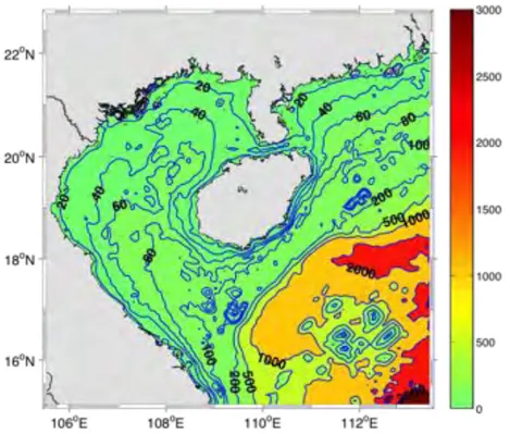
Figure 1.2: Map shows the major topographic features of the Gulf of Tonkin: Isobaths are in meters (m). Data from GEBCO_08.
There are topographic dataset available for the Gulf of Tonkin, like ETOPO2 (global digital bathymetry 2-minute resolution), DEM (digital elevation model 15-minute resolution) from Vietnamese navigation chart, GEBCO_08 (30-second resolution global bathymetry), Smith&Sandwell version 14 (1-minute resolution global bathymetry). GEBCO_08 is chosen here for our simulations because of its higher resolution and the fact that it contains data provided by the International Hydrographic Organization’s (IHO) Member States for shallow water areas shallower than 300m. One of the focuses of IHO’s technical assistance efforts is in the Vietnam East Sea/South China Sea. They contracted a study of shipping traffic patterns in the area and have been assessing the status of hydrographic surveying in the region (according to a report of improved global bathymetry by UNESCO, 2001).
1.2 Tidal forcing
According to Wyrtki (1961), the four most important tidal constituents in the Vietnam East Sea/South China Sea give a relatively complete picture of the tidal pattern of the region and are sufficient for a general description. These tides, with their periods T in hours are shown below in Table 1.1
Table 1.1: List of main tidal constituents
Tide Description Period (hrs)
M2 S2 K1 O1
Semi-diurnal principal solar Semi-diurnal principal solar Diurnal solar
Diurnal principal lunar
12.42 12.00 23.93 25.82
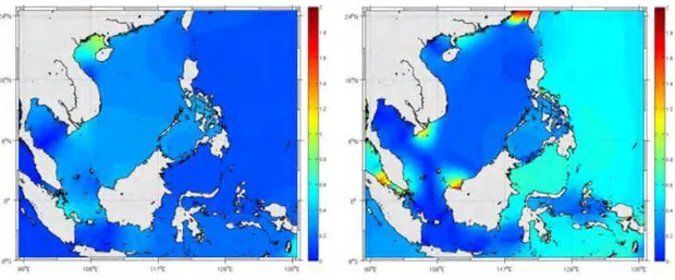
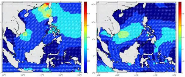
Tides in the Vietnam East Sea/South China Sea have been studied since the 1940s. The co-tidal and co-range charts (maps of tidal phase and amplitudes of the main tidal constituents) that were drawn by various researchers before the 1980s revealed large discrepancies over the shelf areas. The discrepancies among the published charts were reduced since the 1980s, when a number of numerical models were developed to improve the accuracy of tides and tidal current predictions. Recent examples are mostly Chinese: the two-dimensional, depth-integrated shallow water model of Fang et al. (1999) and the three-dimensional tidal models of Cai et al. (2005), Zu et al. (2008) and Chen et al. (2009). Zu et al. (2008) used data assimilation of TOPEX/POSEIDON altimeter data to improve predictions while Cai et al. (2005) explored the sensitivity of shelf dynamics to various model parameters and forcing. With a relatively coarse resolution (quarter degree) model, Fang et al. (1999) and Zu et al. (2008) showed that tides in the Vietnam East Sea/South China Sea are essentially maintained by the energy fluxes of both diurnal and semidiurnal tides from the Pacific Ocean through the Luzon Strait situated between Taiwan and Luzon (Luzon is the largest island in the Philippines, located in the northernmost region of the archipelago). The major branch of energy flux is southwestward passing through the deep basin. The branch toward the Gulf of Tonkin is weak for the semidiurnal tide but rather strong for the diurnal tide. The M2 tidal amplitude is reduced while the O1 amplitude is amplified after they pass through the Luzon strait. The results show that the M2 amplitude is generally small (<0.2m) at the entrance of the Gulf of Tonkin but the K1 and O1 amplitude are about 0.3m (Figure 1.3).
Figure 1.3: Amplitude in meter of O1 (left) and M2 (right) tides in the Vietnam East Sea/South China Sea, from the global tidal solutions FES2004 (Lyard et al., 2006) Vietnamese scientists, e.g., Nguy!n Ng"c Th#y (1984), have also studied tides in the Vietnam East Sea/South China Sea since the 1980s, but the high-resolution dynamics of the Gulf of Tonkin remain poorly estimated. What is known is that the tidal regime of the Gulf of Tonkin is diurnal, with large amplitudes in the north decreasing in the south. Tidal currents are strong and complex. Tides in bays generally have larger amplitudes than in the open ocean but with similar anticlockwise propagation around the coasts (northern hemisphere). The propagation is also much slower consistent with the shallower water. In such small bodies of water, the effects of gravitational forcing acting directly on the water body are small compared with the indirect effects of open-ocean forcing. Therefore, tides in coastal seas and bays are driven primarily by the open ocean tide at the mouth of the bay. In some cases, this can lead to large amplitudes, by at least two processes. One is simply focusing: if the bay becomes progressively narrower along its length, the tide will be confined to a narrower channel as it propagates, thus concentrating its energy. The second process is resonance by constructive interference between the incoming tide and a component reflected from the coast. If the geometry of the bay is such that it takes one-quarter period for a wave to propagate its length, it will support a quarter-wavelength mode at the forcing period, leading to large tides at the head of the bay. Tidal waves enter the Gulf of Tonkin from the adjacent Vietnam East Sea/South China Sea, and are partly reflected in the northern part of the Gulf. The geometry of the basin causes the diurnal components O1 and K1 to resonate. Therefore, the amplitude of these components increases northward along the North Vietnamese coastline, where they reach their highest values in the whole of Vietnam East Sea/South China Sea (exceeding 90 cm for O1 and 80 cm for K1; Fang et al., 1999). The strongest diurnal tidal current occurs in the Hainan Strait.
More specifically, if we consider the Gulf of Tonkin as an ideal rectangular gulf of length L and constant water depth h, which communicates with a deep ocean at the open end, we can compute a solution for resonant modes (Taylor, 1922). For that, we assume that the gulf is sufficiently narrow for the Coriolis force to be neglected, and omit for simplicity the friction effects. In this case, the linear,
non-rotating, one-dimensional shallow water equations (under the assumption that at the closed end of the gulf the normal velocity is vanishing) take a solution in the form of a standing wave:
(1.1) Where Ai is the amplitude at the gulf entrance (x=L), is the frequency of incoming tide, its propagation speed. At the head of the gulf (x=0), the amplitude is . Hence, if cos(kL)=0 for kL =! /2, 3! /2, … (2n-1)! /2,
n=1,2,…, resonance occurs. The first resonance mode (the Helmholtz mode,
generally the most energetic) is associated with the non-dimensional gulf length
kL = !/2, i.e., with gulf length L=!/4 the quarter wavelength, where ! is the length of incoming tidal wave. Thus:
(1.2)
The length of the Gulf of Tonkin is about 500 km and its average depth is 50 m. Therefore the resonance would occur for a tidal forcing period of T = 25.1 hours, which is close to the period of O1 (Fang et al., 1999).
However, neglecting the Coriolis force may not be appropriate (Van Maren et al., 2004). The incoming diurnal tidal waves tend to be deflected to the right by Coriolis forcing and reflect against the northern enclosure of the gulf. The reflected waves propagate southward and are partly dissipated by friction. The result is a mixture of a standing wave, a northward-propagating wave in the eastern part, and a southward-propagating wave in the western part. This suggests a wide range of phase relationships between tidal currents and high/low tides (as opposed to propagating waves, in standing waves currents are out of phase by 90° with water level). Coriolis forcing also produce a frequency shift of the resonant wave. Taylor (1922) and van Dantzig and Lauwerier (1960) proposed a general expression for this frequency shift, again for a rectangular basin. Jonsson et al. (2008) added a useful simplification for narrow bays (if the width is no more than half the length):
(1.3)
W is the width of the basin (270 km for the Gulf of Tonkin) and f is the Coriolis frequency (~0.5 10-4 s-1 at 20°N). The period after correction for rotation is 23.4
hours, which is shorter than the period of O1 and closer to K1. However, we cannot expect the crude estimate of treating the Gulf of Tonkin as a flat-bottomed rectangular gulf to yield an accurate result. We will use our numerical model to provide a better estimate of the optimal resonant period under the influence of complex bathymetry and coastlines and of the Hainan Strait opening in the north.
cos cos i A kx t ! = " ! "=c k ! c= gh ! A=Ai cos(k L) ! " =#c 2L ! " = #c 2L+ 16Wf2 #4 c
1.3 Meteorological conditions
1.3.1 WindsAccording to the literature, dynamical processes in the Vietnam East Sea/South China Sea are governed to a large extent by the Asian monsoon system. In this monsoon system a distinction can be made between the North East (NE) monsoon (also called winter or dry monsoon) and the South West (SW) monsoon (also called the summer or wet monsoon). This system follows the annual cycle (Wyrtki, 1961):
• From September to April the NE monsoon prevails. This monsoon is fully developed in January (8.0 – 10.7 m/s), prevails over the entire Vietnam East Sea/South China Sea. From February onwards, the NE monsoon weakens but prevails until April.
• From May to August the NE monsoon is succeeded by the SW monsoon. During May the NE winds over the Vietnam East Sea/South China Sea collapse and a SW wind succeeds. Its force increases over the following months, reaching full development in July and August (5.5 – 7.9 m/s). From September onwards, however, NE winds occur over the North East Sea and prevail over the entire Vietnam East Sea/South China Sea from October.
This annual cycle is illustrated in Figure 1.4 by monthly-mean wind stress fields for February and August (the NE and SW monsoon highs). These fields are obtained from QuikSCAT monthly climatology. They clearly show the inverted NE and SW monsoon wind directions. Also, it can be observed that during the NE monsoon the wind magnitude is essentially uniform over the entire Vietnam East Sea/South China Sea basin.
Figure 1.4: Monthly-mean surface wind stress for February (left) and August (right). Obtained from Monthly mean wind stress based on the QuikSCAT monthly
Figure 1.5 shows the wind-stress for the Gulf of Tonkin. This data is QuikSCAT monthly climatology and represents the area-averaged conditions over [16°10’– 21°30’N, 105°40’–110°00’E]. A maximum wind stress is observed around December/January, when the NE monsoon is high. A second maximum is observed June/July, when the SW monsoon is high. April/May and August/September are periods of transition between monsoons.
Figure 1.5: Monthly mean wind-stress in the Gulf of Tonkin [16°10’–21°30’N, 105°40’– 110°00’E] from QuikSCAT monthly climatology (2000-2007).
1.3.2 Precipitation
The precipitation in the Vietnam East Sea/South China Sea is mainly controlled by the winter and summer monsoons. Most of the rainfall occurs during the summer monsoon (May-September), in the mountain areas it can reach up to more than 2000 mm (Figure 1.6).
Figure 1.6: Annual mean precipitation [mm/year] from Tropical Rainfall Measuring Mission (TRMM_3B43) observations between 1998 and 2011.
1.3.3 Surface heat flux
The surface net heat flux Qnet is defined as:
1 2 3 4 5 6 7 8 9 10 11 12 −0.1 0 0.1 N/m 2
Qnet = Qsw - Qlw - Qlat - Qsen (1.4)
Qsw and Qlw are the heat fluxes due to solar short wave and long wave radiation
respectively, Qlat is the latent and Qsen the sensible heat flux. The Vietnam East
Sea/South China Sea lies between the equator and the Tropic of Cancer where the incident sunlight is practically vertical to the sea surface. The solar short wave radiation reaches its maximum in April because of the least cloud cover and the vertical incidence of sunlight. In winter Qsw is lowest but due to the tropical
position of the VES/SCS the annual range of values is mild. The latent heat transport Qlat reaches its maximum in winter, due to the strong northeast
monsoon with its cold, dry air. The latent heat flux has minimal during the transition periods between monsoons. As a result, the oceanic net heat gain Qnet
reaches a maximum in April, drops quickly in May and is negative from October to February. The VES/SCS can store a large amount of heat energy and would exert a large influence on the atmospheric circulation and synoptic systems in eastern Asia. The sudden changes of Qsw, Qlat, Qnet in April-May reflect the quick
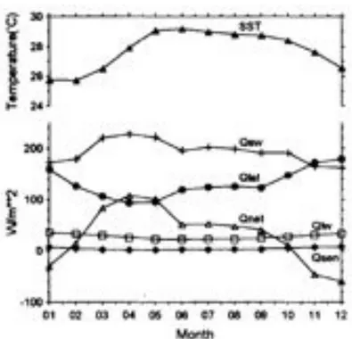
adjustment of atmospheric circulation before the onset of summer SW monsoon. The VES/SCS acts as a source of heat and vapour to maintain the monsoon. It is the water evaporation and convective heating caused by the strong air-sea interactions that influence the local synoptic systems over the VES/SCS. There is also considerable spatial variability. The Gulf of Tonkin in particular is less affected by the summer monsoon winds than southern Vietnam (Figure 1.4). The annual variation of SST in the VES/SCS is lowest in winter and rises swiftly after February (Figure 1.7). SST maximum does not appear in April while the surface net heat flux in the ocean is maximum, but lags by about one to two months. Then the SST drops with the decrease of Qnet. This implies that it is the
surface net heat gain Qnet (not oceanic transport) that drives seasonal SST
Figure 1.7: Annual variations of oceanic heat budget components (W.m-2) and sea surface temperature (oC) averaged over the Vietnam East Sea/South China Sea. (Yang,
1999)
1.4 Ocean Climatology
1.4.1 Sea Surface Temperature patterns
During the NE monsoon (winter), the combined effect of surface heat flux and wind-driven basin-scale circulation contributes to the formation of a tongue of cold water along the northwest coast of the gulf. These processes contribute to seasonal amplitudes of over 6oC in the northwest gulf.
Figure 1.8: Monthly-mean sea surface temperature climatology for Febuary (left) and August (right) from AVHRR Pathfinder Version 5.0/5.1 SST data for 1982-2008. Figure 1.8 shows monthly-mean Sea Surface Temperature (SST) fields for February and August, these months were identified as the maximum of the NE and SW monsoons, respectively. They show that the largest seasonal amplitudes are located in the coastal zones, particularly in the Gulf of Tonkin.
1.4.2 Subtidal circulation
The Gulf of Tonkin is connected to the Vietnam East Sea/South China Sea and has a tropical climate with monsoon winds. It is semi-enclosed with an average water depth of 50 m. During the winter monsoon, the wind blows from the northeast generating a southward flow. During the dry season the southward flow dominates and is described by an anticlockwise rotating cell. During the wet season, the southern monsoon winds are weak in the gulf and become minimal in August. Then, there are two circulation cells, which diverge near the coastline of the Red River Delta.
Figure 1.9: Residual flow in the Gulf of Tonkin during the dry season (February) and the wet season (August), based on the Vietnam National Atlas (1996). The 50, 200, and
Chapter 2: Methods
2.1 Description of the Regional Ocean Modeling System (ROMS)
ROMS (Shchepetkin and McWilliams, 2005) is an evolutionary descendent from the S-Coordinate Rutgers University Model (SCRUM: Song and Haidvogel, 1994), which started as a joint venture between UCLA and Rutgers University oceanographers. From this partnership, two branches of ROMS have emerged. A third version branched from UCLA: ROMS_AGRIF. This version is maintained jointly by IRD (P. Marchesiello, P. Penven and G. Cambon) and INRIA (L. Debreu), which are French institutes working on environmental sciences and applied mathematics. The main originality of this version is its 2 way nesting capability but is otherwise close to the UCLA version regarding the numerical kernel. The model evolution still benefit from frequent exchanges with UCLA (J. McWilliams, A. Shchepetkin, F. Lemarié, J. Molemaker and others) and with a growing body of developers and users of the model. ROMS is briefly presented here with references for further details on numerical schemes and physical parameterizations. Additional information can be found in a series of papers and documents available on the ROMS_AGRIF web site: http://www.romsagrif.org (in the documentation section).
ROMS solves the primitive equations in an Earth-centered rotating environment, based on the Boussinesq approximation and hydrostatic vertical momentum balance. It is discretized in coastline- and terrain-following curvilinear coordinates using high-order numerical methods. ROMS is a split-explicit, free-surface ocean model, where short time steps are used to advance the surface elevation and barotropic momentum, with a much larger time step used for temperature, salinity, and baroclinic momentum. The model has a 2-way, time-averaging procedure for the barotropic mode, which satisfies the 3D continuity equation. The specially designed 3rd-order predictor-corrector time step algorithm allows a substantial increase in the permissible time-step size and a reduction of small-scale numerical dispersion and diffusion. The complete time stepping algorithm is described in Shchepetkin and McWilliams (2005). Associated with the 3rd-order time stepping, a 3rd-order, upstream-biased advection scheme allows the generation of steep gradients, enhancing the effective resolution of the solution for a given grid size (Shchepetkin and McWilliams, 1998). Because of the implicit diffusion in the upstream-biased advection scheme, explicit lateral viscosity is not needed in ROMS, except in sponge layers near the open boundaries where it increases smoothly close to the lateral open boundaries. For tracers, a 3rd-order upstream-biased advection scheme is also implemented for tracers but the diffusion part of this scheme is rotated along isopycnal surfaces to avoid spurious diapycnal mixing and loss of water masses (Marchesiello et al., 2009; Lemarié et al., 2012). A non-local, K-profile planetary (KPP) boundary layer scheme (Large et al., 1994) parameterizes the unresolved physical vertical subgrid-scale processes at the surface, bottom and interior of the ocean. If a lateral boundary faces the open ocean, an active, implicit, upstream biased, radiation condition connects the model solution to the surroundings (Marchesiello et al., 2001). ROMS also include an
accurate pressure gradient algorithm (Shchepetkin and McWilliams, 2003) and a variety of features including air-sea bulk formulae, surface and benthic boundary layers. The model was therefore developed to simulate both coastal and oceanic regions and their interactions. Its computational methods allow for realistic, long-term integrations in a fine-mesh regional domain.
ROMSTOOLS (Penven et al., 2008) is a collection of global data sets and a series of Matlab programs collected in an integrated toolbox, developed for generating the grid, the surface forcing, initial conditions, open boundary conditions and tides for climatologically and inter-annual ROMS ocean simulation.
2.1.1 Equations of continuity and momentum balance
ROMS is a member of a general class of three-dimensional, free surface, terrain-following numerical models that solve the Reynolds-averaged Navier-Stokes equations using the hydrostatic and Boussinesq assumptions. The governing equations can be written in Cartesian coordinates:
(2.1)
(2.2)
(2.3)
with the continuity equation:
(2.4)
The equation of scalar transport is given by:
!T !t +u !T !x +v !T !y+w !T !z =KH !2 T !x2 + !2 T !y2 " # $ % & '+Kz! 2 T !z2 +QT (2.5) !S !t +u !S !x+v !S !y+w !S !z =KH !2S !x2+ !2S !y2 " # $ % & '+Kz !2S !z2+QS (2.6)
The equation of state provides the density fields: !u !t +u !u !x+v !u !y+w !u !w" fv=" 1 ! !p !x+Ax !2u !x2+Ay !2u !y2 +Az !2u !z2 !v !t +u !v !x+v !v !y+w !v !w+ fu=" 1 ! !p !y+Ax !2v !x2+Ay !2v !y2+Az !2v !z2 1 ! !p !z="g !u !x+ !v !y+ !w !z =0
(2.7) Equation (2.1) and (2.2) express the momentum balance in the x- and y- direction, respectively. Equation (2.5) and (2.6) are called the advection-diffusion equations. (u,v,w) are the velocity components in x, y, z-directions (in unit of m/s); t is time (in unit of s), (x,y,z) are rectangular position coordinates in the eat-west, north-south and vertical directions (in unit of m); f is the Coriolis parameter, f =2!sin!, with ! is angular speed of rotation of earth about its axis and ! is geographic latitude; P is dynamic pressure (in unit of Pa), g is acceleration of gravity (in unit of m/s2), T is potential temperature (in unit of oC), S is salinity (in ‰: parts of
thousands), Ax, Ay, Az are kinematic eddy viscosity for x, y, z-directions (in unit of
m2/s); Kx, Ky, Kz are kinematic eddy diffusivity for x, y, z-directions (in unit of
m2/s); QT is temperature (heat) source function (in unit of °C/s); QS is the
contribution of evaporation minus precipitation and river discharge to salt flux (in ‰/s).
2.1.2 Vertical boundary conditions.
The vertical boundary conditions can be prescribed as follows, at the top
(z=!(x, y, t))): Az!u !z " # $ % & ' z=! ="x wind #o (2.8) Az!v !z " # $ % & ' z=! ="y wind #o (2.9) ws=!! !t " us !! !x+vs !! !y (2.10)
where !is surface elevation . The components of the wind-stress vector are given by: !x wind = "airCdU U 2+ V2 and
!
y wind="
airCdV U 2+ V2where !air is air density, Cd is nondimensional wind-drag coefficient with values of the order of 1.1-1.5x10³ , and U, V are horizontal components of the wind vector
measured at a height of 10m above sea level. The surface boundary condition for heat:
!oCPKz !T !z " # $ % & ' z=" =Qt (2.11) !=!(T, S, P)
where !ois surface density; CP is specific heat capacity at constant pressure; Qt is surface total heat flux, the total heat flux consists of the short wave flux (Qsw)
minus the net long-wave radiation (Qlw) and the latent (Qlat) and the sensible heat
fluxes (Qsen): Qt=Qsw-Qlw-Qlat-Qsen. We usually choose to compute Qt using the
surface temperature and the atmospheric fields in an atmospheric bulk flux parameterization (Fairall et al., 2003). This bulk flux routine also computes the wind stress from the wind velocity.
For the salinity flux we consider:
Kz !S !z " # $ % & ' z=! =(E( P)S (2.12)
Where KH is kinematic eddy diffusivity for horizontal direction (x,y); E is
evaporation rate, P is precipitation And at the bottom (z=-H(z,y))
Az!u !z " # $ % & ' z=(H =!x bottom "o (2.13) ! Az"v "z # $ % & ' ( z=) H =*y bottom +o (2.14) Kz!T !z " # $ % & ' z=(H =0 (2.15) Kz!S !z " # $ % & ' z=(H =0 (2.16) !wb+ub "H "x +vb "H "y =0 (2.17)
At the bottom, z=-H(x,y), the horizontal velocity has a prescribed bottom stress which is a choice between linear, quadratic, or logarithmic terms.
us, vs, ws ub, vb, wb are the velocity components at the free surface (z=!) and at the
bottom (z= -H) assuming a slip condition is applied at the base of the water column.
2.1.3 Terrain-following coordinate systems
The advantage of terrain-following vertical coordinates is a natural handling of surface and bottom boundary conditions, which is essential for a proper
representation of flow-topography interactions in regions with complex topography; it also provides greater vertical resolution in shallow water. Following Song and Haidvogel (1994) modified by Shchepetkin and McWilliams (2005), the vertical coordinate is defined as:
z=!(1+")+h."+(h! ho)C("),!1 "" " 0 (2.18) where ho is either the minimum depth or a shallower depth above which we wish
to have more resolution. C(!) is defined as:
C(!)=(1! b)sinh("!) sinh" +b tanh "(!+1 2) " #$ % &'! tanh( 1 2") 2 tanh(1 2") (2.19)
where ! and b are surface and bottom control parameters. Their ranges are
0<! ! 20 and 0! b ! 1, respectively. Equation leads to z=! for ! =!1. Here are some features of this coordinate system:
-It is a generalizations of the traditional ! -coordinate system when ! goes to zero
z=(!+h)(1+")! h (2.20)
-The larger the value of !, the more resolution is given above ho.
-For b=0, refinement is only provides to the surface as !is increased.
-For b=1, refinement is given both to the surface and bottom equally as !is increased.
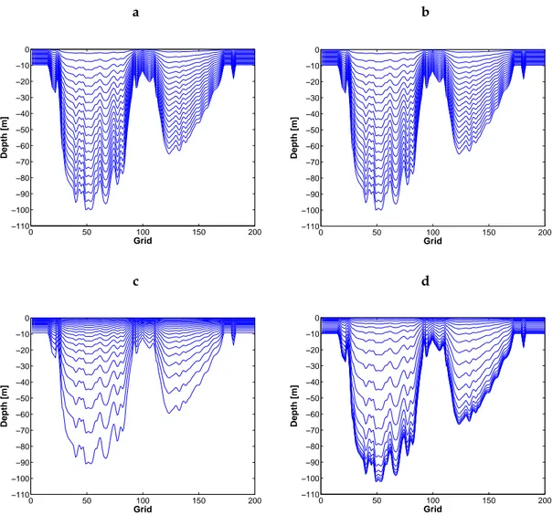
Figure 2.1 shows ! -surfaces for several values of !and b for the same domain. The vertical cell size is:
Hz= !z
!! =("+h)+(h" hc) !C(! )
!! (2.21)
The derivative of C(!)can be computed analytically:
!C(!) !! =(1" b) cosh("!) sinh(") "+b cos h(1 2") 2 cosh2 "(!+1 2) # $% & '( " (2.22)
However, Hz is computed discretely as !z / !! since this leads to the vertical sum
of Hz being exactly the total water depth D.
a b
c d
Figure 2.1: Examples of !-surfaces for the study domain with (a) ! = 0.0001 and b = 0, (b) != 0.0001 and b = 1, (c) ! = 5 and b = 0. (d) != 5 and b = 1.
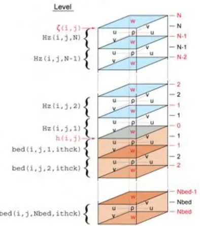
The vertical discretization also uses a staggered finite-difference approximation as shown in Figure 2.2. 0 50 100 150 200 −110 −100 −90 −80 −70 −60 −50 −40 −30 −20 −10 0 Depth [m] Grid 0 50 100 150 200 −110 −100 −90 −80 −70 −60 −50 −40 −30 −20 −10 0 Depth [m] Grid 0 50 100 150 200 −110 −100 −90 −80 −70 −60 −50 −40 −30 −20 −10 0 Depth [m] Grid 0 50 100 150 200 −110 −100 −90 −80 −70 −60 −50 −40 −30 −20 −10 0 Depth [m] Grid
Figure 2.2: Placement of variables on staggered vertical grid. 2.1.4 Horizontal curvilinear coordinates
Orthogonal curvilinear coordinates are used in the horizontal allowing for spherical grids or increased horizontal resolution in regions characterized by irregular coastal geometry. Let the new coordinates be !(x, y) and !(x, y), where
the relationships of horizontal length to the differential distances is given by:
ds
( )
!= 1 m ! " # $ % &d! (2.23) ds( )
!= 1 n ! " # $ % &d! (2.24)Here m(!,")and
n(
!,")
are the scale factors which relate the differential distances (!!,!") to actual (physical) lengths.In the horizontal (!,"), a staggered grid for finite-difference approximate is
adopted with arrangement of variables as shown is Figure 2.3. This is equivalent to the well know Arakawa “C” grid, which is well suited for problems with high horizontal resolution.
Figure 2.3: Placement of variables on an Arakawa C grid
The practice of coastline-following grids was often used in the past in coastal modeling (e.g., the Princeton Ocean Model, POM, applications) in order to improve the accuracy of coastal boundary conditions and limit land masking as much as possible; in the same time, an increase of resolution in coastal areas was possible. However, a major drawback of this technique is the loss of numerical accuracy when cell sizes are uneven and sometimes imperfectly orthogonal. For this reason, ROMS configurations are generally rectangular. In this case, masking out land areas, providing straightforward boundary conditions, represents the coastal boundary (Figure 2.4). Note that these coastal boundary conditions have a limited impact on the solution because in sigma coordinates the coastal areas are very shallow and dominated by bottom rather than lateral friction, i.e., more akin to a natural boundary condition.
2.1.5 Open boundary conditions
Open boundary conditions are more problematic because they constitute an artificial procedure destined to confine the computational domain within the region of interest. It saves computational resources but must be used with care to limit the propagation of boundary condition errors to the interior domain (Marchesiello et al., 2001; Blayo and Debreu, 2005). In ROMS, a combined set of passive (radiative) and active (relaxation to forcing data) open boundary conditions are provided for u, v, T, S and !, following the method of Marchesiello et al. (2001).
Coastal modeling requires well-behaved, long-term solutions for configurations with open boundaries. A numerical boundary scheme should allow the inner solutions to radiate through the boundary without reflection and information from the surrounding ocean to enter the model. The active open boundary scheme implemented in ROMS estimates the two dimensional horizontal phase velocities in the vicinity of the boundary. For each model variable !, the normal (cx) and
tangential (cy) phase velocities are:
cx=! "! "t "! "x "! "x # $ % & ' ( 2 + "! "y # $ % & ' ( 2 (2.25) cy=! "! "t "! "y "! "x # $ % & ' ( 2 + "! "y # $ % & ' ( 2 (2.26)
Radiation conditions are used on all 3D model fields; while open boundary conditions for the free-surface and depth-averaged momentum are given by a Flather-type formulation (Flather, 1976) based on characteristic equations for shallow water models. These barotropic conditions are particularly well suited for tidal modeling as they smoothly allow both tidal forcing and propagation through the boundaries at the same time.
2.1.6 Time-stepping
The model time stepping involves three time levels: current time t, past time t-dt (dt is the time-step), and future time t+dt at which the model fields need to be estimated. For computational economy, the hydrostatic primitive equations for momentum are solved using a split-explicit time-stepping scheme, which requires special treatment and coupling between barotropic (fast/2D) and baroclinic (slow/3D) modes. A finite number of barotropic time steps, within each baroclinic step, are carried out to evolve the free-surface and vertically integrated momentum equations. Fast moving gravity waves such as tides are solved by the
barotropic equations. In order to avoid the errors associated with the aliasing of frequencies resolved by the barotropic steps but unresolved by the baroclinic step, the barotropic fields are time averaged before they replace those values obtained with a longer baroclinic step. The 3D equations are time-discretized using a third-order accurate predictor (Leap-Frog) and corrector (Adams-Moulton) time-stepping algorithm, which is robust and accurate. The enhanced stability of the scheme allows larger time steps, which more than offsets the increased cost of the predictor-corrector algorithm. The 2D mode is advanced using a forward-backward algorithm with also very good numerical properties.
2.1.7 Sigma-coordinate errors: The pressure gradient and diffusion terms
The major advantage of sigma coordinate models is the transformation of the surface and sea bottom to coordinate surfaces. Unfortunately, this is also the source of their major disadvantage: the well-known pressure gradient error that is most acute on steep continental slopes.
In sigma-coordinate, the x-component of the pressure gradient force is determined by: !p !x z=cst =!p !x!=cst "! h !p !! !h !x (2.27)
The first term of the right hand side involves the variation of pressure along a constant ! -surface and the second is the hydrostatic correction. Near steep topography, these 2 terms are large, comparable in magnitude and tend to cancel each other. A small error in computing either term can result in a relatively large error in the resulting horizontal pressure gradient. Beckman and Haidvogel (1993) show that this error is proportional to the slope number: the ratio of topographic variation and topographic depth. They found empirically that this ratio must be lower than a certain threshold (|h(i+1)-h(i)/(h(i+1)+h(i)|) < 0.2; i is the x grid index) to yield acceptable errors (erroneous currents lower than about 1 cm/s). Another source of pressure-gradient error is associated with vertical resolution and is called hydrostatic inconsistency (Haney, 1991). Consistency requires a limit to vertical resolution (given a certain horizontal resolution) but this limit depends on the pressure gradient scheme (Barnier et al., 1998).
The scheme implemented in ROMS is the formulation proposed by Shchepetkin and McWilliams (2003), based on high order density profile reconstruction and re-writing of the equation of state to reduce spurious water compressibility effects on the pressure gradient. This formulation has been designed to minimize truncation errors and is one of the most successful among the large list of schemes proposed in the literature.
Another related problem is that of spurious diapycnal mixing of tracers due to numerical diffusion naturally orientated along sigma surfaces. Spurious mixing produces errors on water masses and currents (due to the geostrophic balance) that can be even more dramatic than pressure gradient errors but much less
attention has been given to the former in the literature. A solution to this problem is to rotate the diffusion tensor (similarly to the pressure gradient but multiple derivatives can be involved) along geopotential surfaces or even better along isopycnal surfaces. Barnier et al. (1998) proposed the first rotated scheme for Laplacian diffusion. Recently, Marchesiello et al. (2009) proposed a new scheme for rotated biharmonic diffusion along geopotential surfaces and Lemarié et al. (2012) completed this scheme for isopycnal surfaces. It is based on a semi-implicit treatment of vertical fluxes, which removes the CFL stability condition, a well know problem for isopycnal diffusion even in climate models.
With robust and accurate corrections to both pressure gradient and diffusion errors ROMS is thus particularly well suited to represent both the continental shelf and ocean dynamics and exchanges across the continental slope
2.1.8 Turbulent closure
The parameterization of unresolved vertical mixing processes in ROMS follows the formulation of Large et al. (1994). It consists of two distinct parameterizations, a non-local, K-profile parameterization (KPP) for surface and bottom boundary layers and an ocean interior scheme. The depth of surface or bottom boundary layers (HBL and HBBL) is determined by equating a bulk Richardson number relative to the surface (or bottom) to a critical value. They thus are strongly dependent on buoyancy and momentum forcing as well as stratification and velocity profiles. In the ocean interior, vertical mixing is regarded as the superposition of 3 processes: vertical shear, internal wave breaking and double diffusion. In addition convective adjustment in case of static instability is provided by a large mixing coefficient. At the interface between boundary layers and the ocean interior, both diffusivity/viscosity and its gradient are forced to match the interior values.
In addition, and this is specific to ROMS_AGRIF, if the surface boundary layer extends to the bottom, we assume that the neutral boundary layer similarity theory holds at the bottom. The bottom boundary condition Az!u !z=" #0 then translates into Az=!u*z (! is the von Karman constant, u* the friction velocity and z is height above the bottom) which serves as a boundary condition for Az. This
gives large improvement to tidal mixing representation in shallow water. 2.1.9 Nesting
ROMS is discretized on a structured grid, so local refinement can be performed via nested grids (i.e., fixed high-resolution local grid embedded in a larger coarse grid). The interactions between the two components are twofold (2-way nesting): the lateral boundary conditions for the fine grid are supplied by the coarse grid solution, while the latter is updated from the fine grid solution in the area covered by both grids (Blayo & Debreu, 1999). The method for embedded gridding takes advantage of AGRIF (Adaptive Grid Refinement in Fortran), a generic coupler with the ability to manage an arbitrary number of embedding levels (as well as adaptive grid refinement, but this feature has not been extensively used).
A recursive integration procedure manages the time evolution for the child grids during the time step of the parent grids. In order to preserve the CFL criterion, for each parent time step the child must be advanced using a time step divided by the coefficient of refinement (e.g., a refinement of 3 for a 5 km grid embedded in a 15 km grid) as many times necessary to match the time of the parent.
2.2 Lagrangian modeling: Ariane
ARIANE (Blanke et al., 1997) is developed in the “Laboratoire de Physique des Oceans” (LPO) in Brest by Bruno Blanke and Nicolas Grima. It is a code that temporally integrates the velocity field to compute trajectories. The package contains the FORTRAN 95 code and Matlab tools for graphic outputs and streamfunction calculation. ARIANE computes trajectories from the 3-dimensional Eulerian velocity field. For that, the velocity field must be interpolated at each particle location along their trajectory. The algorithm is detailed in Blanke and Arhan (1999). It takes advantage of the C-grid used to discretize ROMS equations and provides trajectories for a given velocity field through the computation of 3-dimensional streamlines. The 3 components of the velocity field are known over the six faces of each cell. The non-divergence of the velocity field ensures continuous trajectories within the cell.
ARIANE can be used in two different modes, qualitative and quantitative:
• The qualitative mode uses individual particles to display realistic trajectories. This mode is useful to simulate the trajectory of individual Lagrangian drifters or buoys and assesses the connectivity between various locations. The maximum duration of the particle drift corresponds to the duration of stored data. To initialize the particles in the domain, ARIANE uses five parameters, three spatial ones, a temporal one and a last parameter read but not used in qualitative mode (it is present for consistency with the quantitative mode inputs). The spatial parameters are given in number of cell grid, i.e. we do not indicate longitude, latitude and depth but the corresponding grid cell number.
• The quantitative mode uses thousands or more particles to compute a Lagrangian streamfunction and determine Lagrangian transports. The streamfunction is computed on the horizontal plan of a non-divergent flow, diagnosed by the movement of particles each associated with a weight (volume of water in m3). In this mode, particles are initialized on a section
defined by longitude, latitude and depth limits and intercepted by the same section or different ones. The ensemble of sections must form a closed domain to ensure that a quantitative diagnostic is possible.
2.3 Data for model verification
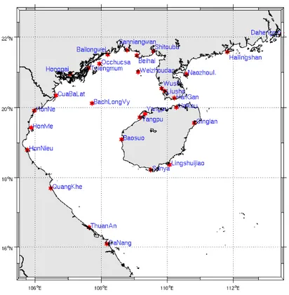
2.3.1 Tide gaugesThe sea surface elevation was recorded at tidal stations along the coast in the Gulf of Tonkin. Data were collected from 30 tidal stations for model verification. The position of these stations is indicated in Figure 2.5. The harmonic constants are taken from the archives of the Institute of Oceanology, Chinese Academy of Sciences, from the British Admiralty Tide and Tidal Stream Tables (Chen et al., 2009). They are generally based on at least one-year observation.
Figure 2.5: The position of the tidal stations for model verification 2.3.2 Altimetry data
Tide gauge measurements have some limitations due to their coastal locations: they describe very shallow water dynamics often biased by local coastal features. In contrast, satellite altimetry provides a global coverage and appears as an efficient way to monitor tidal elevations. With sufficient sampling (5 years and more), estimations of tidal amplitudes are given with an accuracy of a few centimeters.
However, some limitations are associated with the coastal zone, where altimeter observations are often of lower quality. Technically, satellite altimetry is a measure of the travel time taken by a radar pulse to travel from the satellite antenna to the surface and back to the satellite receiver. The use of satellite altimetry observations in coastal regions is limited due to coastal contamination and a discrepancy
between the satellite repeat period and the time scale of sea surface height variability. The treatment of coastal altimetry data used in this study was developed, validated, and distributed by the Centre for Topographic studies of the Oceans and Hydrosphere (CTOH/LEGOS, France). The CTOH is a French Observation Service dedicated to satellite altimetry studies. CTOH developed a processing toolbox, X-TRACK (Roblou et al., 2007) for improved altimeter treatment dedicated for coastal applications. The objective of this processor is to improve both the quantity and quality of altimeter sea surface measurements in coastal regions by applying standard corrections adapted to marginal seas. X-TRACK uses all accurate altimeter missions: Topex/Poseidon (2/11/1992-12/8/2002), Jason-1 (16/1/2002-27/1/2009), Jason-2 (13/7/2008-30/5/2011), Geosat Follow on (8/1/2000-8/9/2008) and Envisat (01/10/2002-14/9/2010). Amplitude and phase lag for each tidal constituent can be locally recovered with CTOH specific harmonic analysis software. In this thesis, apart from 16-year-long continuous record of TOPEX/Poseidon and Jason-1, we used also 5 years of TOPEX-Jason-1 interleaved mission. Interleaved mission means the satellite was shifted on a new orbit (moved longitudinally but keeping the same inclination and cycle length).
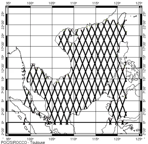
Figure 2.6: Joint TOPEX, Jason 1 and Jason 2 track of primary mission (green lines) and interleaved mission (black lines) in the Vietnam East Sea/South China Sea.
2.4 Harmonic tidal analysis: Detidor
Detidor is a post-processing tool developed at LEGOS for treatment of tidal signals in time series of model and observational data. One of the primary uses of Detidor calculations is to separate out the tidal from the non-tidal components by performing a harmonic tidal analysis. Harmonic analysis is most useful for the analysis and prediction of tidal elevations and currents. The use of this technique for tides appears to have originated with Lord Kelvin (1824-1907) around 1867. A discussion of tidal harmonic analysis can be found in Admiralty manual of Tides (Doodson and Warburf, 1941) and Godin (1972). The harmonic method of analysis treats every tidal record as consisting of a sum of harmonic constituents of known frequency. At time t, the harmonic expression of the ocean tidal height at location
can be written as:
!(",#, t)= Hk k
!
(",#)cos[$k(t)+%k" G(",#)] (2.28)where , are the unknown amplitude and Greenwich phase lag of tide k at location , and and are the amplitude and phase corrections. To avoid the singularities of the amplitude at the amphidromes, it is more common to give equation 2.28 the following form with cosine and sine functions:
!
"(#,$,t)= [Ck
k
%
(#,$)cos(&k(t)+'k)+Sk(#,$)sin(&k(t)+'k)] (2.29)where Ck=Hk cos(Gk) and Sk=Hk sin(Gk).
To account for the nodal correction on the lunar tide, lunar nodal modulation factors are introduced to the harmonic expression of the tidal height (Munk and Cartwright, 1966; Schureman, 1971; Schwiderski, 1980):
!(",#, t)= fkCk k
!
(",#)cos($k(t)+%k+µk)+ fkSk(",#)sin($k(t)+%k+µk)] (2.30)where fk is the nodal factor, µk is the nodal angle. Both of them depend on the position of the lunar node and hence vary slowly with time in the 18.6-year nodal period. For the purpose of solving the unknown amplitude Hk and phase lag Gk
through the least squares estimation procedure.
2.5 Tidal energy budget: COMODO-energy
COMODO-energy is a diagnosis tool developed at LEGOS for calculating the energy budget of the barotropic tides. The energy budget is calculated from tidal atlases (harmonic constant of sea surface elevation and barotropic currents). Here
( , )! "
( , )
k
H
! "
Gk( , )! "
we reintroduce a brief description of the equations. More detailed derivation can be found in Pairaud et al. (2008).
The derivation of the barotropic energy equations are based on the three-dimensional Reynolds-averaged Navier-Stokes equations under the Boussinesq approximation, along with the density transport equation and the continuity equation:
!u
!t+u."u=#2$ % u # g"!+F+D (2.31)
Where F and D are the astronomical forcing and the dissipation:
F=(1+k2! h2)g"#a+g"#LSA (2.32)
D=!.(A!u) "C
H u u" c(!h.u)!h (2.33)
and the continuity equation:
!!
!t +".(Hu)=0 (2.34)
with u the total barotropic current, ! is the sea surface elevation, H is the total water depth, h is the mean water depth (H=!+h), g is the gravitational acceleration, ! is the Coriolis and metrics contribution, k2, l2 are the potential and
deformation Love numbers, !a is the astronomical potential, !LSA is the LSA potential, A is the horizontal momentum diffusion coefficient, C is the quadratic friction coefficient, c is the internal wave drag coefficient.
We can derive the kinetic energy equation by multiplying Equation (2.31) by !Hu and using Equation (2.34):
!ek
!t +".eku=#!gHu.""+!Hu.F+!Hu.D (2.35)
where ekis the kinetic energy per surface unit
ek=1
2!Hu.u (2.36)
lim T!" 1 T 0 #(eku)dt=wp T
$
+wF+wD (2.37)With contributions from pressure gradient, astronomical forcing and dissipation:
wp=! lim T"# 1 T!g Hu.0 $"dt T
%
wF=lim T"# 1 T !0Hu.F dt T%
wD=lim T"# 1 T!0 Hu.D dt T%
(2.38)Using Green’s formula Hu.!!=!.(!Hu)"!!.(Hu)
=!.(!Hu)+!"! "t =!.(!Hu)+1 2 "2 ! "t (2.39)
When integrating Equation (2.39) over a given domain, it is transformed into a flux integral: !!g Hu."" ds #
$
=!!g(1 2 %"2 %t #$
ds+ "Hu.n dl &$
) (2.40)where !g"Hu.n is called energy flux.
The time-averaged domain-integrated energy equation can be expressed as follows: lim T!" 1 T 0
$
%(ek+!g"H )u.n dl= #$
wFds+ T$
wDds #$
(2.41)The mean kinetic energy per surface unit is defined as
ek =lim T!" 1 T 0 ekdt= T
![Figure 1.5: Monthly mean wind-stress in the Gulf of Tonkin [16°10’–21°30’N, 105°40’– 110°00’E] from QuikSCAT monthly climatology (2000-2007)](https://thumb-eu.123doks.com/thumbv2/123doknet/2148139.9133/15.892.284.675.627.974/figure-monthly-stress-gulf-tonkin-quikscat-monthly-climatology.webp)