Image decompositions and transformations as peaks and wells

(1)

HAL Id: hal-00547277

https://hal.archives-ouvertes.fr/hal-00547277

Submitted on 15 Dec 2010

HAL is a multi-disciplinary open access

archive for the deposit and dissemination of sci-entific research documents, whether they are pub-lished or not. The documents may come from teaching and research institutions in France or abroad, or from public or private research centers.

L’archive ouverte pluridisciplinaire HAL, est destinée au dépôt et à la diffusion de documents scientifiques de niveau recherche, publiés ou non, émanant des établissements d’enseignement et de recherche français ou étrangers, des laboratoires publics ou privés.

Image decompositions and transformations as peaks and

wells

Fernand Meyer

To cite this version:

Fernand Meyer. Image decompositions and transformations as peaks and wells. 10th International Symposium on Mathematical Morphology and Its Application to Signal and Image Processing, ISMM 2011, Jul 2011, Verbania-Intra, Italy. pp.25-36, �10.1007/978-3-642-21569-8_3�. �hal-00547277�

(2)

Image decompositions and transformations as

peaks and wells

Fernand Meyer Mines ParisTech, Département maths et systèmes, Centre de Morphologie Mathématique,

F-77305 Fontainebleau Cedex, France

Abstract. An image may be decomposed as a diﬀerence between an image of peaks and an image of wells. Applying a morphological operator to these two components before reconstructing a final image produces interesting filters for grey tone or binary images. This decomposition depends upon the point of view from where the image is considered.

1 Introduction

A binary image is made of particles and holes. Each particle may contain one or several holes and each hole one or several particles. These structures may be deeply nested. For describing this structure, J.Serra [5] introduced the homotopy tree, H.Heijmans [2] called it the adjacency tree. R. Keshet [3] and C. Ballester [1] studied it in depth and gave algorithms for constructing it. They presented also each a diﬀerent extension to grey-tone images of this tree, resulting in the so called tree of shapes.

Here, we propose a description of images which is not as complete as the tree of shapes, but which is extremely simple and fast to construct. Given a reference set X, called view-point set, we decompose an image in a diﬀerence between two components, one representing its peaks, the other its wells. They represent respectively the sums of positive and negative variations of the image if one follows a paths starting in X. Both components belong to the lattice of images without minima outside X, on which we define an adjunction.

Ch.Ronse proposed an identical decomposition for functions defined strictly increasing elements of a poset P, with the final aim to find a sound way for constructing a flat operator on gray level image from a non-increasing operator on binary images [4].

In the present paper we decompose functions along connected paths in graphs. Applying a morphological operator to these two components before reconstruct-ing a final image produces interestreconstruct-ing filters for grey tone or binary images. This decomposition depends upon the point of view from where the image is considered.

(3)

2 Scheduling trains

2.1 Setting the scenario of trains circulating on graphs

Let G = (N, E) be a graph where nodes N and oriented edges or arrows E are weighted with positive weights. The graph may be considered as a railway network, where the nodes are railway stations and the arrows are connections between them. Trains may follow all possible paths on G. However, they may only start from a subset X ⊂ N of railway stations.

Consider a particular train. It starts at station s ∈ X at time τ(s), follows a path θ = (x0 = s, x1, ..., xn= t) where xi and xi+1 are two railway stations

linked by an arrow (i, i+1) of E, weighted by the time ei,i+1needed for following

it. The arrival time at destination is then τ (s) + P

i,i+1∈θ

ei,i+1.

We now consider all trains starting at all possible nodes and taking all pos-sible routes, and observe the earliest time when each node is reached by a train; if a train arrives at i before τ (i), we replace τ (i) by this first arrival time. For some nodes no train ever arrives ; i is such a node, if τ (i) is too early, so that all trains coming from another node arrive at i after τ (i). For others, no train departs: if τ (i) is too late, no train starting from i has a chance to be the first to reach another node ; this is in particular the case if τ (i) = ∞. Some nodes cumulate both situations, and no train departs or arrives.

The resulting shedules_{bτ = Θ}X(e, τ ) depends on the distribution of initial

departure times and crossing times of each edge. Defining τ∞

X by τ∞X = τ on

X and τ∞

X = ∞ elsewhere, it is obvious that ΘX(e, τ ) = ΘN(e, τ∞X), since no

train with an infinite departure time has the chance to reach another node first. ΘN(e, τ∞X) is clearly an opening on the initial distribution of departure times on

all nodes; it is obviously anti-extensive and increasing. It is also idempotent, as a second scheduling would not change the distribution τ (i) any further. We also remark that if τ (s) = 0 for s ∈ X, the resulting schedules simply are the shortest path between X and all other nodes.

2.2 Harmonizing the schedules is a shortest path problem in a completed graph

Completed graph and extended functions We now fix G, e and X and con-sider varying distributions of starting times. Any such distribution is a function defined on the nodes of G. In case of images defined on a grid, G is the graph associated to the grid: pixels are nodes and neighboring pixels are connected by an edge.

We obtain an augmented graph GX, by adding to G a dummy node Ω with

weight τ (Ω) = 0 and dummy edges (Ω, i) between Ω and each node i of X, with eΩi= τi. Since the travelling time along the edge (Ω, i) is τi, it is equivalent for

a train to start from i at time τior from Ω at time 0 and follow the edge (Ω, i)

for reaching i.The earliest time for a train to arrive at any node k of G is the total duration of the shortest path between Ω and k. It follows that scheduling

(4)

3

the graph G amounts to constructing the shortest path between Ω and all other nodes in the graph GX, which is a classical problem in graph theory for which

many algorithms exist. In "Scheduling trains with delayed departures" in the same issue, we have presented the algorithms of Moore Dijkstra and of Berge and shown that, if the introduction of a dummy node Ω and dummy edges (Ω, i) is a useful support for thinking, it is not necessary in practice.

Fig. 1.

Columns 1 and 2 : Binary sets X and Y and their decomposition Column 3 : Xf Y and its decomposition

Column 4 : Xg Y and its decomposition

3 Decomposing an image into peaks and wells

We consider now an image f defined on the the nodes N of the graph G. We define three distributions of edge weights on G and its extension GX, derived

from the distribution of nodes. We consider two nodes i and j of G and a node k ∈ X. The weights of eij in G and of eΩk in GX are:

— e+_ij= f_ij+_{= ∨(f}j− fi, 0) and e+Ωk= fk, positive for upwards transitions and

null otherwise.

— e−_ij= f_ij−_{= ∨(f}i− fj, 0) and e−Ωk= 0 positive for downwards transitions and

null otherwise.

— e#_ij_{= |f}j− fi| = |fij| and e#Ωk = fk> 0.

Consider now an arbitrary node x of G and an arbitrary path π = (Ω, x1,

x2, ..., xn) between Ω and x. We may decompose f (x) along the path π as follows:

f(x) = f(x) − f(xn−1) + f (xn−1) − f(xn−2) + ... + f (x2) − f(x1) + f(x1) −

(5)

Since fj−fi= fij+−fij−for neighboring pixels i, j in the path π, and f (Ω) = 0, we get f(x) = f(x1) + X ij∈π f_ij+₋X ij∈π f_ij−, where x1∈ X is linked to Ω.

Among all possible paths, there is a path_{bπ for which} X

ij∈π f_ij−is minimal. As f (x1) + X ij∈π f_ij+₋X ij∈π

f_ij−has a constant value, the expression f(x1) +

X

ij∈π

f_ij+ is also minimal on_{bπ and so is their sum f(x}1)+

X ij∈π f_ij++X ij∈π f_ij−= f(x1)+ X ij∈π |fij|. f(x1) + X ij∈π f_ij+,X ij∈π f_ij−and f (x1) + X ij∈π

|fij| respectively represent the

pos-itive, negative and total variation along_{bπ in G}X.

The length f (x1) +

X

ij∈π

f_ij+ of the shortest path between Ω and x in the graph G with edge weights e+ _{is the schedule ot the first train arriving at x in}

GX. We write ΘX(e+, f ) for the distribution of schedules on all nodes. Likewise,

the schedules for the distribution of weights e+ and e# are f_X−(x) = X

ij∈π f_ij−= ΘX(e−, f ) and fX#(x) = f (x1)+ X ij∈π f_ij++X ij∈π f_ij−= f (x1)+ X ij∈π |fij| = Θ(f#, f ).

Finally, to each view point X corresponds a decomposition of the function f into a diﬀerence between a function representing the peaks and another repre-senting the valleys: f = ΘX(e+, f ) − ΘX(e−, f ).

4 The lattice of floodings with a unique regional

minimum

The schedulesτ_cX(x) = ΘX(e, τ ) is the length of the shortest path between Ω and

the node x. The edge weights being non negative, there exists a non ascending path between any node and Ω for the valuationsτ_cX. Hence Ω is the only regional

minimum ofτ_cX.

The following formulations are equivalent: — Ω is the only regional minimum ofτ_cX

— the only regional minima of τ belong to X

— τ_cXis invariant by the swamping which imposes Ω as only regional minimum

; that is the flooding Λ+₍_τ_c

X, 0∞Ω), where 0∞Ω is equal to 0 at Ω and ∞

elsewhere.

— _{bτ is invariant by the swamping which imposes the minima of X as only} regional minima ; that is the flooding Λ+₍_{bτ, τ}∞

X)

— considering the threshold at valuation λ, the subgraph spanning all nodes with a valuation τ < λ (we call it the background at level λ) has only one connected component, and this component contains Ω.

(6)

5

We call FX the lattice of all functions verifying the previous equivalent

cri-teria.

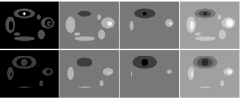
Fig. 2.Decomposition and transformations on binary images

4.1 Infimum and supremum in the lattice FX

FX is a complete lattice, with the ordinary order relations for functions, 0 as

minimal element, ∞ as maximal element.

If h1and h2are two functions of FX, their infimum in FX is simply h1∧ h2.

As a matter of fact, the bakgrounds of h1 and h2 at level λ comprise each

one connected component ; as they both contain Ω, their union, which is the background of h1∧ h2 also consists in one connected component containing Ω.

(7)

Now, h1∨ h2 may have regional minima outside X, which have to be

sup-pressed by swamping. For this reason the supremum h1t h2is equal to Λ+(h1∨

h2; (h1∨ h2)∞X).

Remark: These operators are not distributive one with another.

4.2 An adjunction in the lattice FX

If for each node x we define a neighborhood Vx, the erosion of a function f with

this variable structuring element is εVf (x) = V y∈Vx

fy. This operator is an erosion

both in the ordinary lattice of functions as in the lattice FX. Its adjunct dilation

in the ordinary lattice is δVf (y) = W x∈Vt

y

fx, where Vyt = {x | y ∈ Vx} . Being

an adjunction, they verify for each couple (f, g) of functions the relation: f < εVg ⇔ δVf < g.

As δVf (y) = W x∈Vt

y

fx does generally not belong to FX, the ajunct of εVg is

f

δVf(y) = F x∈Vy−

fx = Λ+(δVf, (δVf )∞X). To establish it we have to prove that

δVf < g ⇔ Λ+(δVf, (δVf )∞X) < g.

On one hand, floodings being extensive we have Λ+_(δ

Vf, (δVf )X) < g ⇒

δVf < g.

On the other hand, if f and g belong to FX., then δVf < g ⇒ Λ+(δVf, (δVf )X) <

Λ+_{(g, g}

X). But Λ+(g, gX) = g, as g is invariant by the flooding Λ+(g, gX).

Concatenating all equivalences, we get for any couple of functions in FX: f <

εVg ⇔ δVf < g ⇔ fδVf = Λ+(δVf, (δVf )X) < g, showing that (εVf, fδVf ) = ( V y∈Vx fy, F x∈Vy− fx) is indeed an adjunction on FX.

Classically εVδfV is then a closing and fδVfεV an opening.

4.3 Razings in the lattice FX

Razings clip peaks and do not create new holes. Thus the image of FX by any

type of razing or reconstruction opening is FX.

5 Min, max and morphological operators through the

decomposition in peaks and wells

Suming up, given a set X, serving as view-point, we are now able to decompose any image f into a cumulative image of its peaks f_X+and a cumulative image of its wells f_X−, such that f = f_X+_{− f}_X−. Both functions belong to FX , a lattice

where we defined a supremum, infimum and an adjunction. Furthermore this lattice is stable by any type of razing.

(8)

7

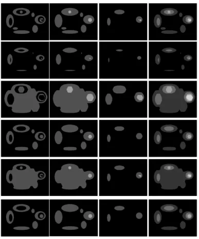
Fig. 3. Decomposition and transformations on binary images. The view point set is the white particle in the first image.

5.1 "Supremum" and "infimum" of two functions

Let (f_X+, f_X−) and (g+_X, g−_X) be the decomposition of two function into peaks and wells, given the view point X. For any composition law 4 on FX, we may define

f 4 g = fX+4 g+X− fX−4 gX−.

Remark: _{We do not necessarily have (f 4 g)}+_X = f_X+_{4 g}_X+ _{and (f 4 g)}−_X= f_X−_4g−_X. This means that the decomposition (f_X+_4g+_X, f_X−_4g_X−) is not necessarily a minimal decomposition of f 4 g.

Based on the operator ∧ and t in FX, we obtain ff g = fX+∧ g +

X− fX−∧ g−X

and fgg = f_X+_{t g}_X+_{− f}_X−_{t g}_X−. Both operators are illustrated by figure 1, where the first row shows in position 1 and 2 the two initial binary sets X and Y, in position 3 their intersection ff g and in position 4 their union f g g. Row 2 presents the image of peaks and row 3 the image of wells. These results are obtained by constructing the decomposition (f_X+, f_X−) and (g+_X, g_X−) which are then combined to obtain ff g and f g g.

5.2 Operators operating on the peaks and wells

Given the decomposition (f_X+, f_X−) of a function f into peaks and wells, and given an increasing operator ψ from FXinto FX, we define bψf = ψ¡f_X+¢−ψ¡f_X−¢. The

decomposition is not necessarily minimal, but since f_X−< f_X+ and ψ increasing, b

ψf will be positive if f is positive.

Figure 2 presents a number of operators on a binary image. The view point set X is the boundary of the image. In each row, the initial image presents a binary image, the second its peaks, the third its wells, and the last the total variation, that is the sum of peaks and wells. Each following row presents a particular transform ψ; we construct ψ¡f_X+¢ and ψ¡f_X−¢ shown in columns 2 and 3. The subtraction bψf = ψ¡f_X+¢_{− ψ}¡f_X−¢gives the resulting binary image in column 1 and the total variation ψ¡f_X+¢+ ψ¡f_X−¢in column 4.

The transforms are presented row wise: 1) initial image; 2) erosion of size 11; 3) dilation of size 15; 4) opening of size 11; 5) closing of size 15; 6) reconstruction opening of size 11.

(9)

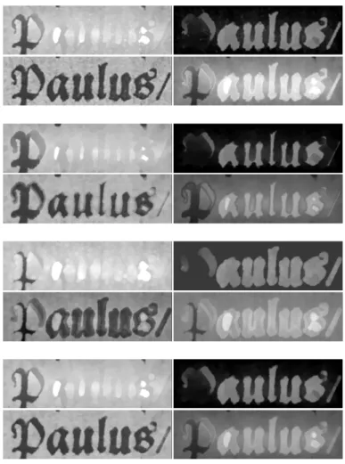
Fig. 4.Decomposition and transformation of grey tone images.

Figure 3 also presents an erosion of size 11 of the same binary image, but the decomposition is made with respect to a diﬀerent view point set X, shown in white superimposition in the first image. X is contained in a white particle, itself contained in a hole contained in a particle. The disposition of the images is the same as for the preceding image. The grey tone scale is artificially enhanced so as to make all structures visible. Let us observe the decomposition. One has to think that the shortest paths start within X until they reach the boundary of the first particle, which appears as a downwards transition. They leave the first hole on an upwards transition, and again leave this particle on a downwards transition. Their paths stay in the background until the other particles are met. The transitions when they enter in the other particles are the same as for a path coming from the boundary of the image. This example shows the utmost

(10)

9

importance of the choice of X. Particles containing X are treated diﬀerently from particles which do not contain it. The second row shows the erosion. As the particles and holes containing X appear as holes both in the peak as in the wells image, their erosion enlarges them. On the contrary, particles and holes not containing X appear as peaks and are indeed eroded. The recomposition bεf = ε¡f_X+¢_−ε¡f_X−¢is shown in image 2.1 and the total variation ε¡f_X+¢+ε¡f_X−¢ in image 2.4.

Fig.4 presents the decomposition and transformation of grey tone images ; there are four groups with an identical disposition. In each group the upper row shows the positive variation σ+ _{and negative variation σ}−_{, whereas the second}

row shows the initial image and the total variation σ#_{. The first group presents}

the initial image and its decomposition. The second group the erosion of size 3, the third the dilation of size 3 and the last the opening of size 3. Since the first letter "P" of "Paulus" intersects the boundary of the image, which plays the role of view point set X, it is not transformed as the other letters.

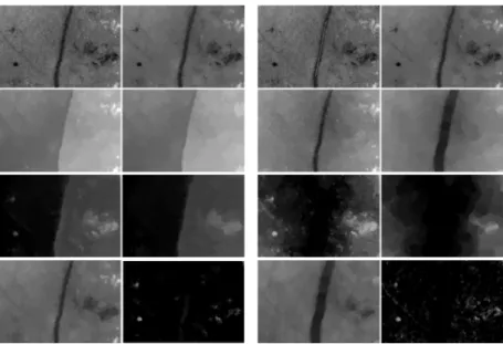
The last example in fig. 5 is taken from an image of the retina. The aim is to detect the small dots and the bloodings without detecting the vessel, although they have the same width. The images are organized as two matrices with the same structure. For the left block the view point set is the left boundary of the image, and for the right block the white segment in superimposition with the vessel in image 1.1 Both blocks are organized as follows. Fig.1.1 the initial image, 1.2 its filtered version which is decomposed. The peaks are in fig 2.1, the wells in fig 3.1. The tranformation applied on peaks and wells in the left block is a reconstruction opening and in the right block an erosion. The final result of the transform is in fig. 4.1. Subtracting image 1.2 from the maximum between 1.2 and 4.1 yields a residue image where the anevrysms are clearly highlighted and the vessel disappeared. Chosing the left boundary of the image as view point X for the left block produces a decomposition where the vessel is split: its right boundary appear in the peak image and its left boundary in the wells image, whereas the microanevrysms appear a dots in the wells image. For this reason, the reconstruction opening leaves the vessel untouched and suppresses the small dots. In the right block, the image is seen from a point view image included in the vessel. For this reason the boundaries of the vessel appear as upwards transitions and the boundaries of the microanevrysms as downward transitions. Like that they completely diverge in the treatment: the vesses is eroded in the peaks image and the dots disappear by eroding the wells image. The recomposed image shows a blown up vessel and suppressed anevrysms.

6 Conclusion

The decomposition we proposed depends on the edge and node weights and upon the point of view, the set X. Changing X produces a diﬀerent decomposition of the same scene, with a diﬀerent distribution of contrast, between the same objects, which may facilitate the segmentation. Changing the edge weights, for instance by keeping only the variations along each edge which are higher than

(11)

Fig. 5.Analysis of the retina in order to detect the micro-anevrysms and discard the vessel

a threshold will put the focus with contrasted contours and ignore the objects with a more fuzzy contour. The distribution of weights on the edges may also be directional, favoring some directions and discarding others. This gives the possibility to analyze anisotropies. The shortest distances which are at the basis of the decomposition may be rendered geodesic. In conclusion, the framework set in this paper should be useful for many tasks in image processing: filtering, segmentation and pattern recognition in general.

References

1. Coloma Ballester, Vicent Caselles, and P. Monasse. The tree of shapes of an image. ESAIM: COCV, 9:1—18, 2003.

2. Henk J. A. M. Heijmans. Connected morphological operators for binary images. Computer Vision and Image Understanding, 73(1):99 — 120, 1999.

3. Renato Keshet. Adjacency lattices and shape-tree semilattices. Image and Vi-sion Computing, 25(4):436 — 446, 2007. International Symposium on Mathematical Morphology 2005.

4. Ch. Ronse. Bounded variation in posets, with applications in morphological image processing, volume 86, pages 249—283. Acta Universitatis Upsaliensis, 2009. Pro-ceedings of the Kiselmanfest.